


1. Introduction
As a ubiquitous phenomenon in daily life, the evaporation of liquids plays a vastly important role in many industrial processes and domestic applications. For example, water desalination and purification by thermal distillation and solar evaporation have potential in mitigating global water scarcity issues (Canbazoglu et al. Reference Canbazoglu, Fan, Vemuri and Bandaru2018; Han et al. Reference Han, Wang, Zuo, Chen, Yuan, Liang, Li, Ajayan, Zhao and Lou2019; Ghim et al. Reference Ghim, Wu, Suazo and Jun2021). Evaporation of liquid coolants is essential for high-power electronic equipment that employ liquid-vapour phase change for thermal management. Typical two-phase cooling devices are the heat pump (Li et al. Reference Li, Zhou, Tian and Li2021a), vapour chamber (Zhou, Liu & Dede Reference Zhou, Liu and Dede2019) and nanoscale evaporators (Vaartstra et al. Reference Vaartstra, Zhang, Lu, Díaz-Marín, Grossman and Wang2020). With the advancement of micro- and nano-technology, more and more designs occur that exploit the liquid evaporation from nanopores. In photothermal membrane distillation, water evaporates on one side of the nanoporous membrane, and vapour flows across the nanopores and condenses on the opposite side (Gong et al. Reference Gong, Yang, Wu, Xiong, Yan, Cen, Bo and Ostrikov2019; Ghim et al. Reference Ghim, Wu, Suazo and Jun2021). In the novel design of a high-flux cooling device, liquids are pumped by capillary force to evaporate through an ultrathin nanoporous membrane to realize highly efficient heat dissipation (Hanks et al. Reference Hanks, Lu, Sircar, Kinefuchi, Bagnall, Salamon, Antao, Barabadi and Wang2020). It is apparent that a fundamental understanding of the nanoporous evaporation could promote the improvement of relevant applications by guiding the material selection and structural design.
For liquid evaporation into air, the diffusion-limited regime was typically considered (Shahidzadeh-Bonn et al. Reference Shahidzadeh-Bonn, Rafaï, Azouni and Bonn2006; Carrier et al. Reference Carrier, Shahidzadeh-Bonn, Zargar, Aytouna, Habibi, Eggers and Bonn2016; Millán-Merino, Fernández-Tarrazo & Sánchez-Sanz Reference Millán-Merino, Fernández-Tarrazo and Sánchez-Sanz2021). In this case, a continuum-based analysis can be applied without invoking molecular dynamics theory. However, as the structural dimension diminishes to nanoscale, gas rarefaction effects have to be accounted for because the molecular mean free path (MFP) is no longer a small quantity (Shen Reference Shen2005). Moreover, the evaporation of liquids into pure vapour has to be described at a kinetic scale due to the presence of a Knudsen layer in the vicinity of the liquid–vapour interface (Schrage Reference Schrage1953; Sone, Ohwada & Aoki Reference Sone, Ohwada and Aoki1989). Researchers have developed analytical and numerical tools to solve the Boltzmann equation for deriving the quantities of interest in evaporation, i.e. the mass flux and the pressure drop (Schrage Reference Schrage1953; Yen Reference Yen1973; Labuntsov & Kryukov Reference Labuntsov and Kryukov1979; Ytrehus & Østmo Reference Ytrehus and Østmo1996; Sone Reference Sone2000). Although complete, these approaches were generally restricted to one-dimensional half-space evaporation problems, which cannot be directly applied to nanoporous evaporation. Other groups considered liquid evaporation in confined tubes or channels at microscale, analysing the thermal and mass transport within the contact line region coupled to the interfacial evaporation (Morris Reference Morris2003; Narayanan, Fedorov & Joshi Reference Narayanan, Fedorov and Joshi2011).
More recently, efforts were devoted to modelling the kinetic evaporation from circular nanopores. The relations between the dimensionless evaporation rate and the driving force (pressure or temperature difference) were attained over a wide range of operating parameters. Lu, Narayanan & Wang (Reference Lu, Narayanan and Wang2015) employed the moment method to solve for the evaporation rate from nanopores. Particularly, they calculated the pore transmissivity using Berman's correlation (Berman Reference Berman1965) to account for the vapour flow resistance in pores. John et al. (Reference John, Enright, Sprittles, Gibelli, Emerson and Lockerby2019, Reference John, Gibelli, Enright, Sprittles, Lockerby and Emerson2021) investigated the nanoporous evaporation by direct simulation Monte Carlo (DSMC) and provided an effective evaporation coefficient approach to handling the nanoporous evaporation using the solution of half-space evaporation problems. Li, Wang & Xia (Reference Li, Wang and Xia2021b) introduced the transitional gas flow formulation into the calculation of vapour flow resistance and extended the nanoporous evaporation model to a wider range of Knudsen numbers. The theoretical studies on nanoporous evaporation dynamics were validated by experimental data since nanoscale manufacturing and measurement became possible (Lu et al. Reference Lu, Kinefuchi, Wilke, Vaartstra and Wang2019; Wang, Shi & Chen Reference Wang, Shi and Chen2020; Xia et al. Reference Xia, Wang, Zhou, Ma and Wang2020).
For practical applications of nanoporous evaporation, one of the most important scenarios is when a liquid surface recedes inside a nanopore. The significance of studying evaporation from a receded liquid meniscus could be multifaceted. In electronics cooling, the receded meniscus is undesirable because it aggravates the risk of dry out (John et al. Reference John, Gibelli, Enright, Sprittles, Lockerby and Emerson2021). Studying the evaporation kinetics of a receded meniscus thus assists in understanding the mechanism of performance degradation when the capillary force fails to balance the viscous pressure drop. In membrane distillation, which employs hydrophobic materials to separate the liquid and vapour, the liquid meniscus is pinned at one end of a nanopore and vapour flows towards the other end (Ghim et al. Reference Ghim, Wu, Suazo and Jun2021). This is an equivalent situation to the case of a receded evaporation surface. Moreover, evaporation of a receded meniscus also occurs in the production of unconventional oil and gas such as shale from nanoscale pores (Jatukaran et al. Reference Jatukaran, Zhong, Persad, Xu, Mostowfi and Sinton2018). It is important to study the phase change of liquid hydrocarbons confined in reservoirs as the pressure drops. However, the evaporation from nanopores with a receded liquid surface is generally less studied in the literature. This is particularly true when we consider the effect of the Knudsen number (Kn) on the evaporation rate. Since the value of Kn may spread over several orders of magnitudes in different applications (Li et al. Reference Li, Wang and Xia2021b), relevant studies are of high significance.
Therefore, this paper focuses on the effects of the Knudsen number on nanoporous evaporation with a receded liquid surface. A semi-empirical model is presented which could predict the liquid evaporation rate from nanopores under different Knudsen numbers. The model is then validated by molecular simulation data using the DSMC method. In § 2 we present a theoretical analysis of the vapour flow in nanopores considering multiple reflections of gas molecules. The vapour densities at either ends of a pore are calculated from the velocity distribution functions. Ultimately, we derive the dimensionless pore transmissivity to solve the Boltzmann equation. In § 3, the DSMC simulation set-up is described, including the domain geometry and the selection of various parameters. In § 4 the theoretical model is validated by simulation results. The characteristics of nanoporous evaporation with receded liquids are examined and comparison is also made with previous models and correlations. Section 5 summarizes the major findings and contributions of the present work.
2. Theoretical analysis
2.1. Vapour flow in nanopores
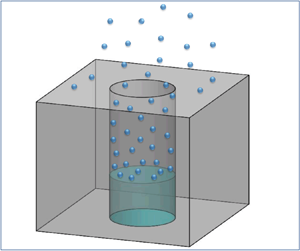
We consider the evaporation of liquid into its saturated vapour from a circular nanopore. The emitted vapour molecules pass through the nanopore and then cross the Knudsen layer until arriving at the far field where vapour is in an equilibrium state. As shown in figure 1, the resistance exerted on the flowing molecules comes from the diffusive reflection on the pore wall and the inter-collisions between molecules. A fully diffusive wall condition is assumed, thus there is a probability that a molecule may not be able to reach the pore outlet from the liquid surface. In addition, other molecules may fail to cross the pore due to collision with surrounding molecules. These two conditions comprise the microscopic explanation of vapour flow resistance in nanopores. The probability that an emitted molecule can reach the pore outlet is referred to as the pore transmissivity or transmission probability (Berman Reference Berman1965; Ota & Taniguchi Reference Ota and Taniguchi1993). Our first purpose is to examine the vapour flow paths under the influence of the pore transmissivity (W) and evaporation coefficient (σ).

Figure 1. Schematic of the diffusive reflection and inter-molecular collisions for vapour flow in a nanopore.
Figure 2 illustrates the trajectory of emitted molecules from the liquid surface. The number of molecules will be discounted by W when reaching the other end of pore, with the rest directing backwards. Meanwhile, the molecules that impinge the liquid surface have a portion σ that is condensed and (1 − σ) that is reflected. Consequently, molecules undergo multiple reflections in the nanopore and the net flux exiting the pore must be found from the summation of series. In figure 2, the molecular flux was depicted by Maxwell's velocity distribution function (VDF), of which the standard form is
 \begin{equation}{f_M}(\rho ,T,\boldsymbol{u}) = \frac{\rho }{{{{(2{\rm \pi} RT)}^{1.5}}}}{\rm exp} \left[ { - \frac{{{{(\boldsymbol{\xi } - \boldsymbol{u})}^2}}}{{2RT}}} \right],\end{equation}
where ρ, T and u are three parameters representing gas density, temperature and macroscopic speed vector, respectively; R is the specific gas constant and ξ is the molecular velocity vector. The VDF of molecules evaporating from the liquid is assumed to be (2.1) with the saturation properties as parameters and without macroscopic speed (Schrage Reference Schrage1953; Ytrehus & Østmo Reference Ytrehus and Østmo1996). Hence, we have
 \begin{equation}{f_L} = {f_M}({\rho _L},{T_L},0),\end{equation}
where TL and ρL are liquid surface temperature and the corresponding saturation density, respectively. The arrows in figure 2 imply the direction in which the VDFs apply. A right arrow means that the VDF applies to positive velocity (ξx > 0) in this one-dimensional problem and vice versa. It can be seen that the components of the VDF exiting the nanopore constitute a geometric series and the summation is easily calculated to be
 \begin{equation}{f_{out}} = {f_L} \cdot \frac{{\sigma W}}{{1 - (1 - \sigma )(1 - W)}},\end{equation}
where the constant of proportionality on the right-hand side of (2.3) is the apparent evaporation coefficient. The value of σ depends on liquid property and temperature (Marek & Straub Reference Marek and Straub2001) and is routinely treated as an input quantity. The pore transmissivity W, on the other hand, depends on the nanopore geometry and the average vapour density in the pore (Karniadakis et al. Reference Karniadakis, Beskok, Aluru, Antman, Marsden, Sirovich, Karniadakis, Beskok, Aluru, Antman, Marsden and Sirovich2005b). Therefore, we need to determine the vapour density in the nanopore during evaporation, as shown in the following text.

Figure 2. The multiple reflections of emitted vapour molecules in nanopores. Here, fL is the VDF corresponding to the liquid surface temperature.
During nanoporous evaporation, backflow of molecules from the far field occurs and this portion of molecules can enter the nanopore via the pore outlet. Figure 3 illustrates the multiple reflection process of backflow molecules. We use fb to denote the VDF of backflow molecules, where ft is a companion of fb. The former is a non-drifted Maxwell VDF at TL and has the same mass flux as the latter, i.e.
 \begin{equation}{f_t} = {f_M}({\rho _t},{T_L},0),\; \quad \int_{{\xi _x} < 0} {{f_t}|{{\xi_x}} |\,\textrm{d}\boldsymbol{\xi }} = \int_{{\xi _x} < 0} {{f_b}|{{\xi_x}} |\,\textrm{d}\boldsymbol{\xi }} .\end{equation}
Figure 3. The multiple reflections of backflow vapour molecules in nanopores. Here, fb is the VDF of the backflow molecules while ft is a companion of fb with the same mass flux.
Equation (2.4a,b) can be understood in the way that some molecules enter the nanopore in the x-direction with their VDF being fb. The same molecules are accommodated by the pore wall and their VDF becomes ft on reaching the opposite pore end. We have assumed that the pore wall and liquid surface have the same temperature and this should be a good approximation for nanoscale pores.
Combining figures 2 and 3, one can find the overall VDF at the liquid surface as well as at the pore outlet
 \begin{gather}{f_{liquid}} = \left\{ {\begin{array}{*{20}{@{}c}} {\dfrac{{\sigma (1 - W){f_L} + W{f_t}}}{{1 - (1 - \sigma )(1 - W)}},\quad \; {\xi_x} < 0\; \; }\\ {\dfrac{{\sigma {f_L} + (1 - \sigma )W{f_t}}}{{1 - (1 - \sigma )(1 - W)}},\; \quad {\xi_x} > 0} \end{array}} \right. \end{gather}
 \begin{gather}{f_{pore}} = \left\{ {\begin{array}{*{20}{@{}l}} {{f_b},}&{{\xi_x} < 0}\\ {\dfrac{{\sigma W{f_L} + (\sigma + W - 2\sigma W){f_t}}}{{1 - (1 - \sigma )(1 - W)}},}&{{\xi_x} > 0} \end{array}} \right..\end{gather}
 Accordingly, the vapour density at the two positions can be attained by integrating the corresponding VDFs over the entire velocity space, such that  $\rho = \mathop \smallint \nolimits^ f \cdot \textrm{d}\boldsymbol{\xi }$.
2.2. Pore transmissivity in the transitional flow regime
The physical significance of pore transmissivity, W, introduced in § 2.1 is the probability that a molecule can pass through the nanopore from one end to the other. In free molecular regime (Kn → ∞), W is a function of only the geometric shape of the wall boundary (Clausing Reference Clausing1932; Davis Reference Davis1960). In the transitional flow regime, additional resistance by molecular inter-collisions is non-negligible and it depends on the average vapour density within the nanopore. Karniadakis et al. (Reference Karniadakis, Beskok, Aluru, Antman, Marsden, Sirovich, Karniadakis, Beskok, Aluru, Antman, Marsden and Sirovich2005b) proposed a transitional flow correlation which links the mass flux and pressure gradient, with the average Kn being a parameter
 \begin{equation}\dot{m}^{\prime\prime} = \frac{{{r^2}\bar{\rho }}}{{8\mu }} \cdot \frac{{\Delta P}}{L}(1 + \alpha \overline {Kn} )\left( {1 + \frac{{4\overline {Kn} }}{{1 + \overline {Kn} }}} \right),\end{equation}
where r and L are the radius and length of the vapour flow domain, respectively; μ and  $\bar{\rho }$ are the viscosity and average density of the vapour. The average Knudsen number
  $\overline {Kn} $ is defined on basis of the average vapour density in the flow domain
 \begin{equation}\overline {Kn} = \frac{\lambda }{r}.\end{equation}
 As shown in (2.8),  $\overline {Kn} $ is defined as the ratio of the molecular MFP to the radius of a nanopore. The MFP (λ) is calculated using the arithmetic average vapour density in the pore; for a variable soft sphere (VSS) model this would be
 \begin{equation}\lambda = \frac{{m{{(T/{T_{ref}})}^{\omega - 0.5}}}}{{\sqrt 2 {\rm \pi}\bar{\rho }d_{ref}^2}},\end{equation}
where m is the molecular mass while Tref, ω and dref are parameters in the VSS model (Shen Reference Shen2005);  $\bar{\rho }$ is the arithmetic average between the vapour density near the liquid surface and at the pore outlet, ρliquid and ρpore. The variable α in (2.7) is a function of
  $\overline {Kn} $ and includes adjustable parameters. Karniadakis et al. (Reference Karniadakis, Beskok, Aluru, Antman, Marsden, Sirovich, Karniadakis, Beskok, Aluru, Antman, Marsden and Sirovich2005b) obtained an empirical expression for α by fitting (2.7) to their DSMC simulation data; α was determined as a combination of inverse tangent and power functions of
  $\overline {Kn} $. We continued this functional form of α in our model calculation with slightly modified parameters, as will be given in the following sections. The use of fitted results for the parameter α determines the semi-empirical nature of our present model.
Equation (2.7) is an extension to Hagen–Poiseuille equation and assumes an isothermal gas flow condition. To extract W from (2.7), we can refer to the kinetic relation  $\dot{m}^{\prime\prime} = P/\sqrt {2{\rm \pi} RT} $, which relates the local vapour pressure and the cross-sectional molecular flux. The net mass flux exiting the pore equals the difference between mass flux at two ends and multiplied by W, i.e.
 \begin{equation}\dot{m}^{\prime\prime} = W({\dot{m}^{\prime\prime}_{liquid}} - {\dot{m}^{\prime\prime}_{pore}}) = W \cdot \Delta P/\sqrt {2{\rm \pi} R{T_L}} ,\end{equation}
where we have assumed an isothermal nanopore with temperature TL. This conforms with the assumption in (2.7), although the molecular VDF at the pore outlet may deviate from a Maxwellian at TL due to non-equilibrium effects. Comparing (2.7) and (2.10) and noting that the viscosity can be expressed as  $\mu = \lambda \bar{\rho }\bar{u}/2$, we get (Li et al. Reference Li, Wang and Xia2021b)
 \begin{equation}W = \frac{{{\rm \pi} r}}{{8L}} \cdot \left( {\frac{{1 + \alpha \overline {Kn} }}{{\overline {Kn} }}} \right)\left( {1 + \frac{{4\overline {Kn} }}{{1 + \overline {Kn} }}} \right).\end{equation}
Therefore, the pore transmissivity is a function of pore size and the average Knudsen number. It is seen that W depends on the average vapour density in a nanopore, while the calculation of vapour density requires the input of W (see (2.5)–(2.6)), thus an iteration procedure is needed to solve the problem.
The result given by (2.11) only applies to infinitely long pores. When the nanopore length, L, diminishes to zero, W tends to infinity rather than the expected unity. This is essentially because the resistance of the pore ends is neglected. The two ends of a circular tube actually exert an additional resistance on the molecular motion whose dimensionless form is simply 1 (Dushman Reference Dushman1922). Therefore, the result of W should be replaced by 1/(1/W + 1/1) to incorporate the effect of the pore ends on the molecular transmission. We have verified this idea using DSMC data in our earlier work (Li et al. Reference Li, Wang and Xia2021b).
2.3. Moment method for Boltzmann equation
From preceding sections, we obtained the average vapour density and transmissivity of the nanopore. To solve the evaporation problem, the important information is the VDF of vapour molecules at the pore outlet, shown in (2.6). The moment method was developed to analytically solve the Boltzmann equation so that the evaporative mass flux can be expressed as a function of the driving force for evaporation, either the pressure or temperature difference between liquid and far-field vapour (Labuntsov & Kryukov Reference Labuntsov and Kryukov1979; Ytrehus & Østmo Reference Ytrehus and Østmo1996). As seen from figure 4, the concept of the moment method is to establish the conservative relations of vapour at three locations: pore outlet, top pore wall and the far field. The molecular VDF at the far field is
 \begin{equation}{f_{far}} = {f_M}({\rho _\infty },{T_\infty },{u_\infty }),\end{equation}
with the parameters in brackets being the thermodynamic properties of the far-field vapour. These parameters are outputs of the evaporation problem. The molecular VDF near the top pore wall is written as
 \begin{equation}{f_{wall}} = \left\{ {\begin{array}{*{20}{@{}l}} {{f_b},}&{{\xi_x} < 0}\\ {{f_M}(\rho^{\prime},{T_L},0),}&{{\xi_x} > 0} \end{array}} \right.\end{equation}
and an auxiliary relation is  $\int_{{\xi _x} > 0} {{f_M}(\rho ^{\prime},{T_L},0){\xi _x}\,\textrm{d}\boldsymbol{\xi }} = \int_{{\xi _x} < 0} {{f_b}|{{\xi_x}} |\,\textrm{d}\boldsymbol{\xi }}$. Therefore, (2.13) implies that molecules impacting on the top pore wall are diffusively reflected and the mass flux is conserved.

Figure 4. Illustration of the three locations occurring in the moment equations.
To this end, the moment equations can be written in a general form
 \begin{equation}\left. {\begin{array}{*{20}{c@{}}} {\varphi \int {{f_{pore}}{\Omega _i}\,\textrm{d}\boldsymbol{\xi }} + (1 - \varphi )\int {{f_{wall}}{\Omega _i}\,\textrm{d}\boldsymbol{\xi }} = \int {{f_{far}}{\Omega _i}\,\textrm{d}\boldsymbol{\xi }} ,\quad \; i = 1,\; 2,\; 3}\\ {\boldsymbol{\varOmega } = {{\big[ {{\xi_x},\; \xi_x^2,\; \; \tfrac{1}{2}{\xi_x}{\boldsymbol{\xi }^2}} \big]}^\textrm{T}},} \end{array}} \right\}\end{equation}
where the three components in vector Ω correspond to the mass, momentum and kinetic energy flux of the vapour molecules, respectively; φ is the porosity of a nanopore or the ratio of pore area to the total area in the plane perpendicular to the x-axis.
So far, the VDF fb has not been specified. We can refer to the work by Ytrehus & Østmo (Reference Ytrehus and Østmo1996) and let  ${f_b} = \beta \cdot {f_{far}}$, where β is part of the output of (2.14). Note that the form of fb is not unique and alternatives can be used without seriously affecting the results (Gusarov & Smurov Reference Gusarov and Smurov2002). We have also assumed that the VDFs in the x-direction at the pore outlet and near the top pore wall are identical; both of them are fb. This point will be validated by molecular simulation in subsequent sections.
3. Molecular simulation by DSMC
3.1. Simulation set-up
The DSMC method was widely adopted to calculate the rarefied gas flow and to provide benchmark data for model validation. We employed the open source software SPARTA to conduct DSMC simulations in this paper (Plimpton & Gallis Reference Plimpton and Gallis2015). Figure 5 shows the computational domain which is an axisymmetric two-dimensional plane containing the nanopore and the ambient space. The dimensions in figure 5 are listed in table 1, which also includes the range of other important parameters. Since the present objective is to study the effect of Knudsen number on evaporation with a receded liquid surface, we did not intensively vary quantities such as porosity, Mach number and the liquid meniscus shape, etc. Instead, we use a simple flat liquid surface with a fixed pore size and porosity. The real meniscus shape of a liquid surface can impact the net evaporation rate from a nanopore. With a concave meniscus in the hydrophilic case, the evaporation rate should be larger than that of a flat surface. Nevertheless, the qualitative trend of the evaporation rate varying with other parameters such as pressure difference and Knudsen number, is not affected by the liquid meniscus shape.

Figure 5. Computational domain for nanoporous evaporation by DSMC.
Table 1. Overview of parameters adopted in present DSMC simulations.

The dimensionless evaporation rate  ${S_\infty } = {u_\infty }/\sqrt {2R{T_\infty }} $ was also maintained at a constant level. Therefore, the purpose is to observe the change of driving force, the pressure ratio between liquid and vapour, under various Knudsen numbers. The control of Kn was done by changing the saturation pressure (or density) of the liquid.
In figure 5, five different boundaries are labelled. Boundary ![]() acts as the liquid surface which emits vapour molecules according to the VDF of
acts as the liquid surface which emits vapour molecules according to the VDF of  $\sigma \cdot {f_L}$. Meanwhile, backscattering molecules can exit boundary
 ![]() at a probability σ when hitting the boundary, with the rest being diffusively reflected back. Boundaries
at a probability σ when hitting the boundary, with the rest being diffusively reflected back. Boundaries ![]() and
and ![]() are fully diffusive with temperature TL. Boundary
are fully diffusive with temperature TL. Boundary ![]() is simply a specular surface which does not affect the evaporation process. The boundary
is simply a specular surface which does not affect the evaporation process. The boundary ![]() is set in such a way that vapour near
is set in such a way that vapour near ![]() has a macroscopic speed u ∞ (John et al. Reference John, Gibelli, Enright, Sprittles, Lockerby and Emerson2021; Wu et al. Reference Wu, Lee, Lee and Wong2001). Since the evaporation problem has only one independent variable, we control the evaporation rate through u ∞ and the results of ρ ∞ and T ∞ will be outputs of the DSMC simulation. This type of boundary condition set-up is routinely adopted in DSMC simulation of kinetic evaporation. We simulated nine different cases to investigate the effect of Kn on nanoporous evaporation and to validate our theoretical analysis in § 2. The cases differ from each other in the values of nL and Lt. With the decrease of vapour density (or increase of Kn), a longer computational domain is necessary to achieve a uniform downstream vapour state. The selection of grid number and time step may also be non-trivial. Table 2 lists all the detailed parameters for nine cases. The grid size was roughly a fraction of the molecular MFP, whereas the time step should be small enough so that a particle may not cross a grid within one calculation step.
has a macroscopic speed u ∞ (John et al. Reference John, Gibelli, Enright, Sprittles, Lockerby and Emerson2021; Wu et al. Reference Wu, Lee, Lee and Wong2001). Since the evaporation problem has only one independent variable, we control the evaporation rate through u ∞ and the results of ρ ∞ and T ∞ will be outputs of the DSMC simulation. This type of boundary condition set-up is routinely adopted in DSMC simulation of kinetic evaporation. We simulated nine different cases to investigate the effect of Kn on nanoporous evaporation and to validate our theoretical analysis in § 2. The cases differ from each other in the values of nL and Lt. With the decrease of vapour density (or increase of Kn), a longer computational domain is necessary to achieve a uniform downstream vapour state. The selection of grid number and time step may also be non-trivial. Table 2 lists all the detailed parameters for nine cases. The grid size was roughly a fraction of the molecular MFP, whereas the time step should be small enough so that a particle may not cross a grid within one calculation step.
Table 2. Detailed parameters used in each simulation case.

In axisymmetric simulations, a radial weighting factor can be applied to even out the density distribution at different radial locations (Bird Reference Bird1994). We tested the use of a radial weighting factor and found that it did make molecules more uniformly distributed in the radial direction. However, the numerical fluctuations became worse and, more importantly, the pressure ratio result was not affected by the use of the radial weighting factor.
The key factor that affects the simulation results is the total number of particles in each case. For the present work, we selected appropriate particle number weightings and the total number of particles ranges from 1.6 to 3.6 million. Increasing the particle number is beneficial in yielding accurate results as well as in reducing numerical fluctuation. Cases with a large number of grids will consume vast computational resources if the particle number is increased. Hence, there is a trade-off in selecting the grid number and the particle number. All the simulations were run on a desktop computer with 5 processors and the CPU frequency was 2.9 GHz. The calculation time was between 12 and 36 h for each simulation case.
3.2. Data reduction
The simulations were first run for 70 000 steps to reach a steady state. We judge the steady state by examining the evolution of particle number with time. It was found that the total particle number barely changed after 50 000 steps, thus the pre-stage simulation should be sufficient. Subsequently, the calculation was conducted for another 100 000 steps to generate the samples. We sampled the distributions of pressure, density, temperature and macroscopic speed in the domain every 5 steps, so that a total of 20 000 samples were attained for each run. The number of samples was verified to be large enough and a further increase of sample number did not change the arithmetic average or standard deviation much.
Using the SPARTA code, one can directly output information such as pressure, temperature or density in each grid. Besides these results, we also extracted the molecular VDF at different locations. The molecular VDF was calculated from the ‘snapshot’ of the flow field which includes the spatial coordinates and velocity components of all molecules at a given moment. For a specified location, the VDF of ξx can be written as
 \begin{equation}{f_x} = \frac{{m\sum\limits_{i \in (\Delta V \cap \Delta {\xi _x})} {{N^i}} }}{{\Delta V \cdot \Delta {\xi _x}}},\end{equation}
where m is the molecular mass,  $\Delta V$ and
  $\Delta {\xi _x}$ are the volume elements surrounding the location of interest and the x-velocity interval, respectively; Ni = 1 represents the ith molecule that is within the volume element
  $\Delta V$ and whose
  ${\xi _x}$ is within the interval
  $\Delta {\xi _x}$. The calculation of the VDF was also performed over the 20 000 samples and the results were numerically averaged. For VDFs of ξy and ξz, (3.1) can be used in an identical manner.
4. Results and discussion
4.1. Flow field
As an example, figure 6(a) displays the vapour density contour of case 1, which has the largest density and smallest Kn among all the cases. It is seen that the vapour density continuously decreases from the liquid surface down to the far field. The pattern of the density distribution in figure 6(a) represents the picture for all the other cases, albeit with different domain lengths. We also observed that the variation of density primarily occurs in the nanopore. Outside the nanopore, the density is more uniform. This is confirmed in figure 6(b), which plots the vapour density along the symmetry axis. Ninety per cent of the overall vapour density drop is caused by the nanopore. Therefore, the vapour flow resistance in the nanopore has a fundamental influence on the evaporation process when the liquid surface recedes into the pore. A sophisticated analysis of the vapour flow dynamics in the nanopore as done in § 2 is indispensable and provides insights into the governing factors of nanoporous evaporation.

Figure 6. DSMC simulation results of case 1: vapour density contour (a) and the density distribution along the x-axis (b).
The red diamond in figure 6(b) corresponds to the saturated vapour density,  ${\rho _L} = m \cdot {n_L}$. It is evident that the density near the liquid surface is lower than the saturation level. Due to the non-equilibrium feature of kinetic evaporation, temperature and pressure jumps across the liquid-vapour interface have been widely studied in the literature (Fang & Ward Reference Fang and Ward1999; Hu & Sun Reference Hu and Sun2016). The circular data marker in figure 6(b) shows the density near the liquid surface calculated by our model (2.5). Note that the calculation of ρliquid involves solving the Boltzmann equation such as (2.12)–(2.14). In this way, ρ ∞ and T ∞ are obtained and the results of fb and ft are also known. We see that the present model has captured well the density discontinuity across the liquid surface. The vapour density at the pore outlet was also calculated, and the result is slightly higher than the simulation data. This is probably due to the selection of fb, which is subject to substantial uncertainties (Gusarov & Smurov Reference Gusarov and Smurov2002). Another observation is that the vapour density almost linearly changes in the nanopore, except near the liquid surface, where a relatively fast drop occurred due to end effects. The quasi-linear distribution of vapour density supports the use of the arithmetic average between
  ${\rho _{liquid}}$ and
  ${\rho _{pore}}$ to calculate
  $\overline {Kn} $.
In figure 7, the total particle number of case 1 is plotted against simulation time. The curve remains flat, with slight fluctuations after approximately 30 000 steps, which proves the sufficiency of the selected 70 000 steps as the pre-stage simulation. The inset of figure 7 shows the distribution of vapour density along the y direction in the far field, that is, at x = 1×10⁻⁶ m and at different y coordinates (see figure 6a). It is important that the vapour density remains constant with y, as shown in the inset, so as to ensure the correctness of the simulation set-up in terms of the domain length, Lt.

Figure 7. Variation of total particle number with simulation time for case 1. The inset shows the vapour density distribution in the y direction at the far field.
The vapour density fields under various average Kn in the nanopore are compared in figure 8. It is clear that the density fields exhibit a similar variation pattern regardless of Kn. With the increase of Kn, a longer simulation box was required to obtain a uniform density distribution at the far field. In figure 8, the domains of case 5 and case 9 are only partially displayed for convenience of comparison. A closer examination of the contours may reveal some qualitative differences among the three cases. For case 1, with high vapour density and low Kn, the contour lines within the nanopore are not perfectly flat, i.e. the flow has a certain two-dimensional character. This feature gradually disappears in case 5 and case 9, with the enhancement of Kn. The contour lines of case 9 are largely parallel to the liquid surface, except for a small region near the entrance. In case 9, the vapour flows in the free molecular regime and inter-molecular collisions can be neglected. Molecules tend to be evenly distributed in the radial direction within the nanopore. As Kn gets smaller, the flow regime becomes that of transitional flow and the vapour gradually exhibits a viscous property. Under such conditions, the boundary slip effects (Karniadakis et al. Reference Karniadakis, Beskok, Aluru, Antman, Marsden, Sirovich, Karniadakis, Beskok, Aluru, Antman, Marsden and Sirovich2005a) or the inner friction force between molecules may add to the two-dimensional feature.

Figure 8. The vapour density contours at different average Kn in a nanopore. For case 5 and case 9 the domain is partially displayed.
John et al. (Reference John, Gibelli, Enright, Sprittles, Lockerby and Emerson2021) reported the existence of Moffatt eddies near the top pore wall at a lower porosity (0.25) and Kn (0.05). They concluded that the one-dimensionality of vapour flow tends to break down with small porosity and low Kn. Their findings are consistent with our results, which indicate the difficulty in modelling nanoporous evaporation with small porosity and high vapour densities. We also note that John et al. (Reference John, Gibelli, Enright, Sprittles, Lockerby and Emerson2021) employed a plane two-dimensional geometry for simulation, while the present work utilizes an axisymmetric domain which better reflects the shape of nanopores.
4.2. Molecular VDF
The VDF of molecules is the basis of the kinetic analysis of gas flow. All the macroscopic quantities of gases can be found from the integration of the VDF (Shen Reference Shen2005). In § 2.3, we assumed that the vapour has a same VDF at the pore outlet and near the top pore wall in the x-direction, which is fb. Here, we validate the assumption using the calculated VDFs from DSMC simulation. For this purpose, we sample a series of coordinate and velocity files at different time steps. Two small volume elements are then selected at the pore outlet and near the top pore wall, as shown in the inset of figure 9(a). The velocity space in the x-direction is equally divided into a number of intervals. All the molecules located in the selected volume elements are marked and then grouped according to the velocity intervals. In this way, we obtained the VDFs at two locations of interest under different values of Kn. The results are presented in figure 9(a–c), which includes the three cases: 1, 5 and 9. The abscissa is the velocity component in the x-direction and the ordinate is the corresponding probability distribution function;  ${f_x} \cdot \Delta {\xi _x}$ equals the mass density of molecules whose
  ${\xi _x}$ is within the range of picked
  $\Delta {\xi _x}$. In figure 9, all results were calculated using (3.1) with a velocity interval
  $\Delta {\xi _x} = 40\;\textrm{m}\;{\textrm{s}^{ - 1}}$.

Figure 9. Molecular VDFs at the pore outlet and near the top pore wall under different values of Kn. Three cases are considered: case 1 (a), case 5 (b) and case 9 (c). The ratio of moments at the two locations is calculated and shown in (d) for the different cases.
The non-drifted Maxwell VDF is plotted in figure 9(a–c) for comparison, and is shown by solid black lines. The density and temperature parameters were extracted from the flow field at pore outlet. First of all, we see that the left-half VDF  $({\xi _x} < 0)$ at the two locations agree well with each other under different Kn. The data scatter of cases 5 and 9 is more intractable due to the increased rarefaction degree. However, the VDFs at two locations basically overlap on the left half, with a minimal exception in case 9 around
  ${\xi _x} = 0$. The results generally corroborated our assumption used in developing the theoretical model. Second, the left-half VDFs have a positive drift compared with the solid line, which is because the backflow molecules came from the far field. Vapour at the far field has a uniform macroscopic speed which is u ∞. In the present simulations, the dimensionless parameter S ∞ is fixed at 0.06 and the downstream speed u ∞ is approximately 31 m s−1. The right-half VDF at the pore outlet also has a positive drift relative to the solid line, which is interesting because molecules just emitted from a liquid surface should have no drift speed. It is possible that the diffusive reflection by the pore wall and inter-collisions have worked to yield a drift speed in the vapour. Finally, we found that the right-half VDF near the top pore wall is non-drifted; the data match the solid line closely. This is expected because all the incident molecules were accommodated by the top pore wall and were re-emitted in a diffusive way so their velocity was fully regenerated.
To further demonstrate the analogy between VDFs at the pore outlet and near the top pore wall in the x-direction, we calculated moments over the VDFs from ξx = −∞ to ξx = 0. Figure 9(d) plots the ratio of moments at the two locations for three cases where f 1 and f 2 correspond to the pore outlet and the top pore wall, respectively. The three moments selected were  $\Omega = [1,{\xi _x},\xi _x^2]$. It is seen that the moment ratios at two locations are close to unity, meaning that the VDFs in the x-direction are close to each other for the two locations. The disparity increases with the case number, i.e. the Knudsen number; this may be partially due to the larger data scatter at higher Knudsen number. Nevertheless, the maximum deviation is seen to be only 10 % even when
  $\overline {Kn} $ is as large as 14.5.
4.3. Pressure ratio  ${P_\infty }/{P_L}$

After delving into the flow field and VDF of nanoporous evaporation, we now proceed to the pressure ratio between the far field and the saturation pressure at TL. Since the net evaporation of liquid is driven by the difference between the saturation pressure and the ambient vapour pressure, the ratio of the two is of practical interest. Figure 10 shows the results of the pressure ratio for all the nine cases with varied Kn. When given an evaporation rate, we solve the Boltzmann equations (2.12)–(2.14) along with the expression for the pore transmissivity W. As a result, we are able to find the vapour density and pressure at the far field, and thus the pressure ratio can be determined. The locations of the pressures referred to are illustrated in the inset. We note that PL is not the vapour pressure near the liquid surface; it is the saturation pressure corresponding to TL and nL  $({P_L} = m \cdot {n_L}R{T_L})$. Due to non-equilibrium effect of net evaporation, the vapour pressure near the liquid surface is smaller than PL, just as for the vapour density discontinuity observed in figure 6(b). The simulation data are represented by red triangles in figure 10 and the error bars are a standard deviation over time steps. Therefore, the errors indicate the degree of data oscillation with simulation time. This type of error is usually larger than that from running parallel cases and comparing the averaged results. By further adding to the total particle number in the simulation, the oscillation error could be diminished to a lower level.

Figure 10. Pressure ratio between the far field and saturation changing with average Kn. The DSMC simulation results are compared with the present model as well as to the correlations developed by Berman and John et al.
It is seen from figure 10 that the pressure ratio decreases with Kn, first at a faster rate which then gradually approaches a constant. For a fixed evaporation rate, a larger value of  ${P_\infty }/{P_L}$ means a smaller evaporation resistance, thus the evaporation process becomes easier as the Kn gets smaller. This trend may be counterintuitive if we consider the fact that additional flow resistance from inter-molecular collisions is introduced with decreasing Kn. Consequently, the evaporation resistance should rise as Kn decreases, in contrast to present results. In fact, the relative proportion of wall collisions and inter-molecular collisions must be considered to understand the observed variation trend. When Kn is large or when the flow is in the free molecular regime, 100 % of molecules experience the diffusive wall collision which is the dominant transport mechanism. With the decrease of Kn, more molecules travel by inner-collisions and the proportion of wall collisions significantly reduces. The present results imply that diffusive wall collision is less efficient than inter-molecular collision in transporting the fluid. The pressure ratio
  ${P_\infty }/{P_L}$ actually has a similar variation trend to the pore transmissivity W, with Kn (see (2.11)). An increase in W directly enhances the pressure ratio for a fixed evaporation rate, or improves the evaporation rate for a fixed pressure ratio. The behaviour of transmission probability under different flow regimes has been widely investigated in the literature (Ota & Taniguchi Reference Ota and Taniguchi1993; Karniadakis et al. Reference Karniadakis, Beskok, Aluru, Antman, Marsden, Sirovich, Karniadakis, Beskok, Aluru, Antman, Marsden and Sirovich2005b). Although these studies were not conducted in the context of nanoporous evaporation with a receded liquid surface, the results are qualitatively consistent with the present work. The results in figure 10 reveal the important effects of the Knudsen number on nanoporous evaporation with a receded liquid surface. By altering the governing mechanism of vapour transport in a nanopore, Kn could ultimately influence the evaporation resistance. Care should thus be taken in the design of nanoscale evaporators which may operate in the receded liquid condition. The fluid property and system pressure level could be key parameters for consideration as they determine the value of Kn.
The predicted results by the present model are plotted in figure 10 and a good agreement is observed between the model and DSMC data. For model calculation, the kernel function α in (2.7) was determined as  $\alpha = 0.73{\tan ^{ - 1}}(4{\overline {Kn} ^{0.8}})$, which was motivated by the work of Karniadakis et al. (Reference Karniadakis, Beskok, Aluru, Antman, Marsden, Sirovich, Karniadakis, Beskok, Aluru, Antman, Marsden and Sirovich2005b). We also calculated the pressure ratio using two different sources for pore transmissivity. Berman (Reference Berman1965) proposed the classic correlation for free molecular transmissivity which can be used with the moment method to solve the Boltzmann equation. The corresponding result for the pressure ratio is independent of Kn and agrees with the asymptotic value of the simulation data. John et al. (Reference John, Gibelli, Enright, Sprittles, Lockerby and Emerson2021) developed an empirical correlation based on simulation data which can predict the apparent evaporation coefficient given the porosity, meniscus shape, receded height and the intrinsic evaporation coefficient. For our cases, the intrinsic evaporation coefficient was unity and a flat meniscus was considered. The dimensionless receded height should be 2.5 based on its definition and the porosity 44.4 %. Substituting all the inputs into the correlation, the obtained pressure ratio is given in figure 10. As the mentioned correlation did not include Kn, the result was similarly for the free molecular regime. However, the dashed line in figure 10 deviates from the asymptotic value of the DSMC data, which is attributed to the two-dimensional plane geometry of the simulation domain in John et al. (Reference John, Gibelli, Enright, Sprittles, Lockerby and Emerson2021). The evaporation resistance in the two-dimensional plane geometry was seen to be smaller than that in an axisymmetric geometry with the same aspect ratio of the nanopore. Therefore, the use of an axisymmetric geometry is necessary to authentically reflect the characteristic of nanoporous evaporation.
We also simulated the nanoporous evaporation with varied evaporation coefficient (σ) and demonstrated the validity of our model under a wider parametric range. Figure 11 plots the dimensionless pressure ratio with the evaporation rate (S ∞). Three values of σ were selected and the evaporation rate increased from 0.06 to 0.21. In these cases, the temperature and saturation density of the liquid surface are fixed, while the evaporation rate is varied by changing the value of u ∞. The error bars represent the data fluctuation with simulation time, similar to those in figure 10. An excellent agreement is observed between the DSMC data and our model under different evaporation coefficients and rates. It can be concluded that the present semi-empirical model has a good capability in predicting the nanoporous evaporation rate with varied Knudsen number and evaporation coefficient.

Figure 11. Validation of the present model for varied evaporation coefficient (σ) and evaporation rate (S ∞) using DSMC data.
In future work, it is planned to extend the parameter ranges of DSMC simulation to cover different nanopore size, evaporation coefficient, porosity and evaporation rate under various Knudsen numbers. The obtained data base would be fruitful in systematically validating the theoretical analysis in this paper.
5. Summary and conclusions
We reported a theoretical and numerical investigation on the evaporation of liquids receding inside a nanopore. The evaporation problem was solved through the Boltzmann equation with the moment method. A sophisticated analysis of vapour flow in the nanopore was conducted considering the multiple reflections of vapour molecules. The theoretical model was validated by molecular simulation using the DSMC method. Results of flow field, molecular VDF and the pressure ratio were obtained and the effects of Knudsen number on evaporation resistance were discussed.
For nanoporous evaporation with a receded liquid surface, it was found that the vapour flow resistance in the nanopore played a major role in determining the evaporation rate. Up to 90 % of the total vapour density drop was within the nanopore in the present simulation cases. The theoretical model accurately captured the density discontinuity across the liquid–vapour interface. The molecular VDFs at the pore outlet and near the top pore wall were the same in the x-direction, which corroborated the assumption used in theoretical analysis.
For the pressure ratio between the far-field vapour and the saturation value of the liquid surface, the result was observed to decrease with Knudsen number. It can be concluded that the evaporation resistance gradually increased as the Knudsen number became larger. In the free molecular regime (Kn > 10), the evaporation resistance reached an asymptotic level without further change. The variation trend of the pressure ratio can be explained by the relative proportion of diffusive wall collisions and inter-molecular collisions, the latter being more efficient for molecular transport. The present work revealed the important effects of the Knudsen number on nanoporous evaporation with a receded liquid surface. The vapour flow dynamics in the nanopore is critical to the theoretical analysis. We finally suggest that the use of an axisymmetric simulation domain is desirable in nanoporous evaporation studies.
Funding
This work was supported by National Natural Science Foundation of China (No. 51976002 & 51776007).
Declaration of interests
The authors report no conflict of interest.


