


1. INTRODUCTION
As of 1994, the International Global Navigation Satellite System (GNSS) Service (IGS) has guaranteed high-quality GNSS data products that allow open access to the conclusive global reference frame for scientific, educational, and commercial applications. (Beutler, Reference Beutler2000). The IGS, part of the Global Geodetic Observing System, runs a global network of GNSS ground stations, data centres, and data analysis centres to offer data, and products procured from the data, that are necessary for Earth science studies; multi-disciplinary Positioning, Navigation, and Timing (PNT) applications and learning. In addition, IGS offers Global Positioning System (GPS) satellite ephemerides and clock products with various accuracies for divergent requirements. Some research and analysis of GPS or GNSS satellite ephemerides and clock products have been recently performed. Such research shows that orbits determined from ephemeris do not coincide with real GPS satellite orbits. Some reference stations were implemented to determine the orbits by the algorithm of inverse GPS, which means that the reference stations were regarded as satellites and satellites as receivers (Nomura et al., Reference Nomura, Tanaka and Yonekawa2007). A report suggested evaluating the accuracy of the IGS final GPS orbits to examine their precision and accuracy. A restricted quantity of laser ranging tracking data was accessible and was implemented to examine the complete dependability of the IGS accuracy approximations (Griffiths and Ray, Reference Griffiths and Ray2009). After the significant accomplishments of GPS and GLONASS (Angrisano et al., Reference Angrisano, Gaglione and Gioia2013), novel navigation constellations, such as Galileo, BeiDou (BDS), Quasi-Zenith Satellite System (QZSS), and the Indian Regional Navigation Satellite System (IRNSS) were developed by Europe, China, Japan, and India.
The quality evaluation of precise ephemeris and clock products for novel navigation constellations was focused, and Precise Point Positioning (PPP) examinations were performed to additionally substantiate the standard of the Multi-GNSS Experiment (MGEX) precise ephemeris and clock products (Guo et al., Reference Guo, Li, Zhang and Wang2016). The Galileo In-Orbit Validation Element (GIOVE)-A carrier phase examination has been linked with GPS measurements to gain the greatest precision of orbit determination. The accuracy of the GIOVE-A satellite clock solution was at the ns-level, but in contrast with the GPS satellite clock results, the GIOVE-A satellite clock bias grew rapidly with time (Su and Zimmermann, Reference Su and Zimmermann2009). The precise GPS satellite orbit and clock offered by IGS were examined for applications in maritime precise positioning. The outcomes reveal that it was necessary to abbreviate real-time IGS interval products for more precise positioning solutions (Cho et al., Reference Cho, Jeong and Park2010).
IGS MGEX is geared toward gathering data and examination of all accessible satellite navigation systems. The ephemeris and clock quality of the Galileo products of the four MGEX analysis centres for 20 weeks were analysed. The exactness examined by satellite laser ranging residuals was at the one decimetre level with a systematic bias of about −5 cm for every analysis centre (Steigenberger et al., Reference Steigenberger, Hugentobler, Loyer, Perosanz, Prange, Dach, Uhlemann, Gendt and Montenbruck2015). Observation data sets from three divergent periods and 23 IGS stations across the globe were handled in static mode with four free online PPP services. Computation revealed that the precision of the daily solutions for the northern and eastern components estimated by the four online PPP services can achieve millimetre level accuracy, the exactness of ellipsoid elevation (H) can reach 1–2 cm, and the accuracy of the Zenith Tropospheric Delay (ZTD) estimation outcomes was about 1–2 cm (Guo, Reference Guo2015).
The performance of IGS Real-Time Service (RTS) products in PPP was studied by starting with a comprehensive description and evaluation of IGS RTS products. The outcomes revealed that IGS RTS products in real-time PPP can reduce the solution Root Mean Square (RMS) error by about 50% when contrasted with the solution gained from the forecasted portion of the IGS ultra-rapid products (Elsobeiey and Al-Harbi, Reference Elsobeiey and Al-Harbi2016). An exhaustive performance analysis was conducted between the independent single-system method and the two-step GPS-assisted method for precise orbit determination of BDS. The outcomes showed that for the BDS Inclined Geosynchronous Orbit (IGSO) and Medium Earth Orbit (MEO) satellites, the two-step GPS-assisted method outperformed the independent single-system method in internal orbit overlap precision and external satellite laser ranging validation. For BDS Geosynchronous Earth Orbit (GEO) satellites, the two methods had similar performances (Lou et al., Reference Lou, Liu, Shi, Wang, Yao and Zheng2016).
GPS positioning can be severely degraded in challenging GPS surroundings. Multi-sensor integration positioning and correlation algorithms have been designed to further improve the trustworthiness and accessibility of GPS for measurement work. It is recognised that integrating GPS and INS can deliver an enhanced performance over the individual systems (Angrisano et al., Reference Angrisano, Petovello and Pugliano2010). However, the performance of GPS/Inertial Navigation System (INS) integrated positioning and measurement will be seriously degraded in challenging GPS environments. Some studies have been carried out to fuse Ultra-Wide Bandwidth (UWB) with GPS or INS (Jiang et al., Reference Jiang, Petovello, O'Keefe and Basnayake2012, Petovello et al., Reference Petovello, O'Keefe, Chan, Spiller, Pedrosa and Basnayake2010), which would return more precise GPS positioning in trying surroundings. In this research, the PPP/INS/UWB tightly coupled positioning among various precise satellite ephemeris and clock products are compared and evaluated. Final, rapid and ultra-rapid products are applied in PPP/INS/UWB tightly coupled positioning, respectively. The paper is divided into five sections. Following this introduction, we provide an overview of the observation model of PPP. Section 3 describes PPP/INS/UWB tightly coupled positioning. Test results are then presented and analysed in Section 4, followed by a summary of the main conclusions.
2. OBSERVATION MODEL OF PRECISE POINT POSITIONING
The traditional PPP observation model, including the pseudorange, carrier phase and Doppler measurements, can be written as (Du and Gao, Reference Du and Gao2010):
 $$L=\rho+c\cdot (dt-dt_s)+d_{ion}+d_{trop}+M_L+\varepsilon_L$$
 $$\varPhi=\rho+c\cdot (dt-dt_s)-d_{ion}+d_{trop}+\lambda N+M_{\varPhi}+\varepsilon_{\varPhi}$$
 $$D=\dot {\rho }+c\cdot (\delta dt-\delta dt_s )-\skew4\dot{d}_{ion} +\skew4\dot{d}_{trop} +\varepsilon _D$$
where L, Φ and D are the pseudorange, carrier phase and Doppler measurements, ρ is the geometric distance as a function of the receiver and satellite coordinates, ρ̇ is the geometric range rate, c is the speed of light in a vacuum, dt s and dt are the satellite clock error and receiver clock error, δ dt s and δ dt are the satellite clock error drift and receiver clock error drift. d ion and ḋ ion are the first-order ionospheric delay and ionospheric delay drift, d trop and ḋ trop are the tropospheric delay and tropospheric delay drift. M L and M Φ are the multipath errors of the pseudorange and carrier phase measurements and ε L, εΦ and εD are a combination noise of the pseudorange, carrier phase and Doppler measurements. The tropospheric delay d trop is modelled at the zenith and is mapped using a mapping function to the satellite elevation. The Niell mapping function is used in this case.
Table 1. GPS Satellite Ephemerides / Satellite & Station Clocks.

Using real-time precise GPS orbit and clock products enables uncertainties in the satellite orbit and clock corrections to be significantly reduced. The additional error sources, such as the satellite antenna phase centre offset, phase wind up, Earth tide, ocean tide loading, and atmosphere loading can be eradicated with the correction model. The widely used ionospheric-free combination uses the GPS frequency dispersion property to mitigate the first-order ionospheric delay effect. The observation model of the ionospheric-free combination can be written as (Du and Gao, Reference Du and Gao2010):
 $$L_{if}={f_1^2 \over f_1^2-f_2^2}\,L_1-{f_2^2 \over f_1^2-f_2^2}L_2=\rho+c\cdot (dt-dt_s)+d_{trop}+M_L+\varepsilon_L$$
 $$\Phi_{if}={f_1^2 \over f_1^2-f_2^2}\Phi_1-{f_2^2 \over f_1^2-f_2^2}\Phi_2=\rho+c\cdot (dt-dt_s)+d_{trop}+\lambda_1N_{if}+M_{\Phi}+\varepsilon_{\Phi}$$
 $$D_{if}={f_1^2 \over f_1^2-f_2^2}D_1-{f_2^2 \over f_1^2-f_2^2}D_2=\dot{\rho}+c\cdot (\delta dt-\delta dt_s)+\skew4\dot{d}_{trop}+\varepsilon_{D}$$
where the subscript if denotes the ionospheric-free combination observation.
Because the change of tropospheric delay is very slow, the tropospheric delay drift can be neglected in this case. The variables estimated here include three positional parameters, the receiver clock error, the receiver clock error drift, the zenith tropospheric delay, and the ionospheric-free carrier ambiguity.
The IGS gathers, records, and distributes GPS observation data sets of that are of sufficient exactness to fulfil the objectives of a broad span of applications and experiments. These data sets are evaluated and integrated to create the IGS products shown in the table below (Cho, et al., Reference Cho, Jeong and Park2010).
3. PPP/INS/UWB TIGHTLY COUPLED POSITIONING
3.1. System State Model
The system error dynamic model of integrated navigation used in the Kalman filter is developed based on the INS error equations. The insignificant terms are neglected in the process of linearization (Titterton and Weston, Reference Titterton and Weston2004). The psi-angle error equations of INS are as follows (Li et al., Reference Li, Chang, Gao, Wang and Hernandez2016):
 $$\delta \dot{{\bi {r}}}=-{\bf \omega}_{en}\times \delta {\bi {r}}+\delta {\bi {v}}$$
 $$\delta \dot{{\bi {v}}}=-(2{\bf \omega}_{ie}+{\bf \omega}_{en})\times \delta {\bi {v}}-\delta{\bf \psi}\times {\bi {f}}+{\bf \delta}$$
 $$\delta \dot{{\bf \psi}}=-({\bf \omega}_{ie}+{\bf \omega}_{en})\times \delta{\bf \psi}+{\bf \varepsilon}$$
where δr, δv and δψ are the position, velocity and orientation error vectors, respectively. ωen is the rate of navigation frame with respect to earth, and ωie is the Earth rate with respect to an inertial frame.
The accelerometer bias error vector δ and the gyro drift error vector ε are regarded as the random walk process vectors, which are modelled as follows:
 $$\dot{{\bf \delta}}={\bf u}_{\delta}$$
 $$\dot{{\bf \varepsilon}}={\bf u}_{\varepsilon}$$
where uδ and uε are white Gaussian noise vectors.
The receiver clock, tropospheric delay and ionospheric-free carrier ambiguity state dynamic equations can be written as (Abdel-Salam and Gao, Reference Abdel-Salam and Gao2001):
 $$\delta\skew4\dot{d}t=\delta dt+u_{dt}$$
 $$\delta\skew4\dot{d}t=u_{\delta dt}$$
 $$\dot{d}_{trop}t=u_{trop}$$
 $$\dot{N}_{if}=0$$
where u dt, u δ dt and u trop are the white Gaussian noise vectors of the receiver clock error, the receiver clock error drift and the zenith tropospheric delay, respectively.
By combining Equations (7) to (15), the system state model becomes, in a matrix and vector form:
 $$\dot{{\bi X}}={\bi \Phi}{\bi X}+{\bi u}$$
where X is the error state vector, Φ is the system transition matrix, and u is the process noise vector.
3.2. Observation Model
The GPS observation model in the PPP/INS/UWB tightly coupled architecture is composed of the pseudorange, carrier phase and Doppler difference vectors between the GPS observation and the INS predication value (Zhang and Gao, Reference Zhang and Gao2008):
 $${\bf Z}_{{\rm GPS}}= \left[ \matrix{ L_{j}^{{\rm GPS}}-L_{j}^{{\rm INS}} \cr \Phi_{j}^{{\rm GPS}}-\Phi_{j}^{{\rm INS}} \cr D_{j}^{{\rm GPS}}-D_{j}^{{\rm INS}} \cr \vdots }\right]$$
where  $L_{j}^{{\rm GPS}}$,
  $\Phi_{j}^{{\rm GPS}}$ and
  $D_{j}^{{\rm GPS}}$ are the ionospheric-free pseudorange, carrier phase and Doppler value observed by the j th GPS satellite, respectively.
  $L_{j}^{{\rm INS}}$,
  $\Phi_{j}^{{\rm INS}}$ and
  $D_{j}^{{\rm INS}}$ are the ionospheric-free pseudorange, carrier phase and Doppler values of the j th satellite predicted by INS, respectively.
The observation model of UWB information is composed of the range difference between the UWB observation and the INS predication range (Li, et al., Reference Li, Chang, Gao, Wang and Hernandez2016):
 $${\bf Z}_{{\rm UWB}}= \left[\matrix{ r_i^{{\rm UWB}}-r_i^{{\rm INS}} \cr \vdots } \right]$$
where  ${r}_{i}^{{\rm UWB}}$ is the UWB ranging measurements of the i th UWB unit and
  $r_{i}^{{\rm INS}}$ is the distance calculated via the coordinates estimated using INS and the coordinates of the UWB reference stations.
Corresponding to the system state model, the generic measurement equation of the Kalman filter can be written as:
 $${\bi Z}_k={\bi H}_k{\bi X}_k+{\bi \tau}$$
where Zk is the m-dimensional observation vectors, Hk is the observation matrix, and τ is the measurement noise vector with covariance matrix Rk, assumed to be white Gaussian noise. When a UWB signal is available, the filter observation Zk includes the GPS measurement ZGPS and UWB measurement ZUWB, otherwise, the observation Zk only includes the GPS measurement.
The accuracy of the position and velocity calculated by INS decreases with time. The data update rate of GPS receivers and UWB are configured as 1 Hz. The pseudorange, carrier phase and Doppler values predicted by INS maintain reasonably high accuracy over a second. Therefore, a linear model for GNSS and UWB measurements is used with first order Taylor series truncation. It is undeniable that the feasibility of the linear model would present a challenge to filter convergence in PPP/INS/UWB tightly coupled positioning. The nonlinearity in the observation equation due to a tightly coupled algorithm and the lever arm effect can result in a major error under some harsh conditions. Sigma Point Kalman Filters (SPKF), such as the Marginalised Unscented Kalman Filter (MUKF), have been proven to be effective methods to address the nonlinearity problem in the measurement equations (Chang, Reference Chang2014).
On the basis of the system state model and the observation model, the Kalman filter serves to fuse information in integrated navigation. The optimal estimation of the state vector from the Kalman filter can be reached through time and measurement updates (Han et al., Reference Han, Wang, Wang and Tan2015). In a closed loop integration scheme, a feedback loop is used for correcting the systematic errors and the error states will be reset to zero after every measurement update. In this way, the assumption of small errors can be employed (Nassar and El-Sheimy, Reference Nassar and El-Sheimy2006).
3.3. PPP/INS/UWB Tightly Coupled Positioning
Figure 1 illustrates the architecture of the proposed PPP/INS/UWB tightly coupled positioning system. The INS mechanisation algorithm obtains the present position, velocity and attitude solutions from the measurements of the Inertial Measurement Unit (IMU). The position and velocity information can be additionally gathered with the pseudorange and Doppler measurements from the GPS receiver. After undergoing quality control, and with the ephemeris of the GPS satellites, the position and velocity from the INS mechanisation algorithm are implemented in the forecasting of the pseudorange, carrier phase, and Doppler measurement outcomes. During prediction of the carrier phase, the float ambiguity value that resolved in the previous epoch is used. The precise ephemeris and clock products are utilised in the computation of the precise satellite position and the clock correction. After correcting for the errors in the raw GPS measurements, the corrected pseudorange, carrier phase, and Doppler measurements from the un-differenced GPS are input with the INS-predicted measurements into the Kalman filter. Simultaneously, given the base station position, the position from the INS mechanisation algorithm is used to predict the range value of the UWB. The UWB measurements are likewise input with the INS-predicted measurements into the Kalman filter. The filter estimation values are combined and updated by the Kalman filter to gain the final position, velocity and attitude.

Figure 1. PPP/INS/UWB tightly coupled positioning.
4. DATA ANALYSIS
Field tests were conducted to evaluate the performance of the proposed scheme on the roof of the Nottingham Geospatial Institute (NGI). Figure 2 shows the electrically powered (battery) locomotive and test track that is located on the roof. The track is a total of 120 m in length with a 184·15 mm gauge. The locomotive can house a multitude of sensors, which provides a multi-sensor platform. It can be utilised for various dynamic tests (Stephenson et al., Reference Stephenson, Meng, Moore, Baxendale and Edwards2011). The test consists of one Micro-Electro-Mechanical System (MEMS) grade IMU, one tactical grade IMU, three UWB units, and two GPS receivers. The sampling rate of the UWB unit was 1 Hz. At the start, a Leica AS10 GNSS dual-frequency antenna was installed on the top of a pillar above the NGI locomotive and a UWB unit was fastened under the antenna with a known lever-arm. Two UWB units were set on the pillars on the NGI roof and the coordinates of the pillars were known. The distance  $r_{1}^{{\rm UWB}}$ and
  $r_{2}^{{\rm UWB}}$ between the locomotive and the pillars were measured by UWB. This UWB unit was also connected to a laptop to store the range observations. The MEMS IMU inside the locomotive was connected to the Leica antenna and recorded raw observations onto a Secure Digital (SD) card for post-processing. Another GPS receiver was set on one of the pillars on the NGI roof to act as the reference station. As the UWB ranges were time tagged by the laptop system time, the laptop was synchronised to the GPS time to collect 1 Hz UWB ranges prior to the test. The sampling rate of GPS receivers and INS were respectively configured as 1 Hz and 200 Hz.

Figure 2. The electric locomotive and test track (Stephenson et al., Reference Stephenson, Meng, Moore, Baxendale and Edwards2011).
The whole period of the test was about 20 minutes. PPP/INS/UWB tightly-coupled positioning was realised by the program of multi-sensor integrated positioning developed by our research team. GPS observations were processed using GPS software GrafNavTM 8·0 in Differential GPS (DGPS) mode and the solution was regarded as the position and velocity reference. The attitude reference was generated by Inertial Explorer processing software using observations from two GPS receivers and one tactical grade IMU. The specifications of the MEMS-IMU are given in Table 2. The experienced trajectory and the devices used during tests are presented in Figure 3. The sky plots (azimuth versus elevation) of GPS at the moving station are shown in Figure 4. The Geometrical Dilution Of Precision (GDOP) value variation during the experimental period is illustrated in Figure 5. The GDOP value of the GPS is greater than 1 and the maximum value approaches 2.
Table 2. MEMS grade IMU technical data in field test.


Figure 3. Field test trajectory and instruments.

Figure 4. Sky plots (azimuth vs. elevation) for GPS.

Figure 5. Dilution Of Precision (DOP) value variations during the experimental period.
In data processing, the initial parameters of the Kalman filter for the integrated positioning were finalised based on experience. The initial position and velocity errors were set based on the precision of the initial data from the GPS. The initial position errors were 1 m, 1 m, and 2 m, and the initial velocity errors were 0·1 m/s, 0·1 m/s and 0·5 m/s in North-East-Down (NED) directions, respectively. The transfer alignment method was implemented to gain attitude data to eschew initial alignment errors that hindered the navigation results of various schemes. The initial platform alignment errors were 0·01°, 0·01° and 0·1°. Based on the measurement accuracy of the IMU, the initial standard deviations of gyro and accelerometer biases were 15°/h and 600 mg, respectively. The initial standard deviation of pseudorange, carrier phase, Doppler and UWB observations were 2·5 m, 0·03 m, 0·1 m/s and 0·3 m using their prior statistical data. All the parameters are uniform for all schemes to achieve a valid comparison of performance (Li et al., Reference Li, Chang, Gao, Wang and Hernandez2016).
4.1. PPP/INS/UWB Tightly Coupled Positioning with Final Products
4.1.1. Tightly coupled positioning in the full GPS coverage environment
In order to test the improvement of UWB on PPP/INS tightly-coupled positioning in the full GPS coverage environment, PPP/INS integration (scheme 1) and PPP/INS/UWB integration (scheme 2) with final products are tested and compared. Figure 6 shows the field test trajectory comparisons between the reference value and PPP/INS tightly coupled positioning with the final products. Figure 7 shows the time series of position errors in the northern and eastern directions. Position errors were calculated based on the reference position to examine the performance. Table 3 demonstrates the RMS values and the Maximum (MAX) values of the position error and the velocity error. When the final satellite ephemeris and clock product is implemented, the PPP/INS tightly coupled positioning can gain an accuracy of 0·394 m and 0·430 m in the northern and eastern coordinate components, respectively. Simultaneously, the RMS of the velocity errors were 0·172 m/s and 0.117 m/s, respectively.

Figure 6. Field test trajectories of PPP/INS integrated positioning with final products in the full GPS coverage environment.

Figure 7. Position error and velocity error of PPP/INS integrated positioning with final products in north and east directions: (a) position error; (b) velocity error.
Table 3. RMS of position error and velocity error in north and east directions for PPP/INS.

The field test trajectory comparisons between the reference value and PPP/INS/UWB tightly coupled positioning in the full GPS coverage environment (scheme 2) are shown in Figure 8. Figure 9 shows the time series of position errors. The RMS value and the MAX value of the position error and the velocity error are listed in Table 4. When GPS data is available, the PPP/INS/UWB tightly coupled positioning can achieve an accuracy of 0·245 m and 0·295 m in the northern and eastern coordinate components, respectively. It can be shown that the UWB is able to improve the position accuracy of PPP/INS tightly coupled positioning by 38% and 21% in the north and east directions. Compared with scheme 1 (0·383 m), the Two-Dimensional (2D) position error from scheme 2 is increased to 0·583 m. This clearly illustrates that the UWB observation is very helpful in tightly coupled positioning.

Figure 8. Field test trajectories of PPP/INS/UWB integrated positioning with final products in the full GPS coverage environment.

Figure 9. Position error and velocity error of PPP/INS/UWB integrated positioning with final products in north and east directions: (a) position error; (b) velocity error.
Table 4. RMS of position error and velocity error in north and east directions for PPP/INS/UWB.

4.1.2. Tightly coupled positioning in the partial GPS coverage environment
In order to clearly observe the impact of UWB on PPP/INS tightly-coupled positioning during GPS blockage, PPP/INS integration (scheme 3) and PPP/INS/UWB integration (scheme 4) with final products are tested and compared under the condition that three GPS satellites are available between 486,150 s and 486,550 s and two GPS satellites are available between 486,550 s and 486,950 s. Figure 10 shows the field test trajectory comparisons between the reference value and PPP/INS tightly coupled positioning with the final products in the partial GPS coverage environment (scheme 3). Figure 11 shows the time series of position errors in the northern and eastern directions. Table 5 demonstrates the RMS values and the MAX values of the position errors and the velocity errors. When the GPS signal is less available, the accuracy of PPP/INS tightly coupled positioning reaches 1·437 m in the north and 2·618 m in the east directions, respectively. Velocity accuracy of about 0·254 m/s in the north and 0·282 m/s in the east directions is achievable.

Figure 10. Field test trajectories of PPP/INS integrated positioning with final products in the partial GPS coverage environment.
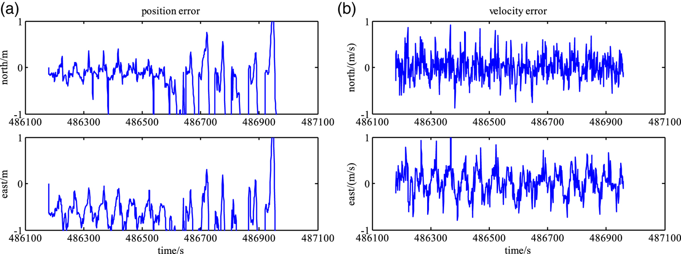
Figure 11. Position error and velocity error of PPP/INS integrated positioning with final products during GPS blockage in north and east directions: (a) position error; (b) velocity error.
Table 5. RMS of position error and velocity error in north and east directions for PPP/INS.

Figure 12 shows the field test trajectory comparisons between the reference value and PPP/INS/UWB tightly coupled positioning in environments where GPS signal reception is limited or impossible (scheme 4). Figure 13 shows the time series of position errors. Table 6 summarises the RMS and MAX values of the position and velocity errors. As shown in the figures and the table, the PPP/INS/UWB tightly coupled positioning can achieve an accuracy of 0·623 m and 0·470 m in the northern and eastern coordinate components, respectively. When compared with scheme 3, the positional accuracies in the north and east directions are improved by 57% and 78%, respectively, for scheme 4. The largest position errors in the north and east directions are 6·669 m and 9·411 m, respectively, when scheme 3 is used. In contrast, the largest corresponding position errors when scheme 4 is applied are 3·711 m and 2·307 m, respectively. Compared against PPP/INS integration, the PPP/INS/UWB tightly coupled positioning achieves a higher position accuracy in a partial GPS coverage environment. Two UWB stations acting as pseudolites which provide more accurate range information, makes the observation model function better and improves the space distribution structure of observation. The UWB observations effectively restrain the divergence when GPS data is less available. The role of UWB in tightly coupled positioning is much larger in the partial GPS coverage environment than that in the full GPS coverage environment.

Figure 12. Field test trajectories of PPP/INS/UWB integrated positioning with final products in the partial GPS coverage environment.

Figure 13. Position error and velocity error of PPP/INS/UWB integrated positioning with final products during GPS blockage in north and east directions: (a) position error; (b) velocity error.
Table 6. RMS of position error and velocity error in north and east directions for PPP/INS/UWB.

4.1.3. Tightly Coupled Positioning with final products from different institutions
To assess the performance of PPP/INS/UWB tightly-coupled positioning with precise orbit and clock products from various analysis centres, the products from IGS, the Centre for Orbit Determination in Europe (CODE), the German Research Centre for Geosciences (GFZ), the Centre National d'Etudes Spatiales (CNES) and Wuhan University (WHU) are collected and used. Figures 14 and 15 show the RMS values of the position and velocity errors from several analysis centres. As shown in the figure, the final products from IGS and CNES show the best agreement at the 0·2–0·3 m level in the north and east directions. The RMS of position accuracy in the north and east directions among CODE, GFZ and WU are 0·4–0·5 m in general, suggesting agreement to within a few decimetres for PPP/INS/UWB tightly coupled positioning.

Figure 14. Position error of PPP/INS/UWB integrated positioning with final products from different institutions in north and east directions.

Figure 15. Velocity error of PPP/INS/UWB integrated positioning with final products from different institutions in north and east directions.
4.2. PPP/INS/UWB Tightly Coupled Positioning with Rapid Products
The difference between final products and rapid products for PPP/INS tightly coupled positioning is compared to the difference for PPP/INS/UWB tightly coupled positioning to test the impact of UWB on the integrated positioning system. Figure 16 shows a comparison of field test trajectories between reference value and PPP/INS tightly coupled positioning with rapid products (scheme 5). The time series of position errors in the northern and eastern directions are shown in Figure 17. RMS and MAX values of position errors and velocity errors are demonstrated in Table 7. Compared with the PPP/INS tightly coupled positioning with final products, the position accuracy in the north and east directions are reduced by 15% and 10% for scheme 5, respectively.

Figure 16. Field test trajectories of PPP/INS integrated positioning with rapid products.
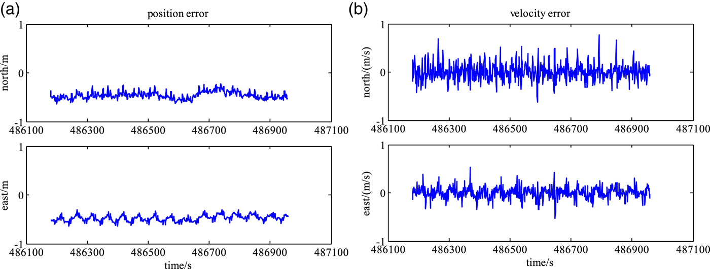
Figure 17. Position error and velocity error of PPP/INS integrated positioning with rapid products in north and east directions: (a) position error; (b) velocity error.
Table 7. RMS and MAX of position error and velocity error in north and east directions for PPP/INS.

Figure 18 shows a field test trajectories comparison between the reference value and PPP/INS/UWB tightly coupled positioning with rapid products (scheme 6). Figure 19 shows the time series of position errors in the northern and eastern directions for tightly coupled positioning with rapid products. Table 8 demonstrates RMS and MAX values of position and velocity errors. Scheme 2 and scheme 5 achieved a close performance. The position error of scheme 5 is slightly larger than the position error of scheme 2, which suggests the tightly coupled positioning with the final products has greater precision. The largest position errors in the north and east directions are 1·039 m and 0·766 m, respectively, when scheme 2 is used. In contrast, the largest corresponding position errors when scheme 6 is applied are 1·075 m and 0·767 m, respectively. The accuracy of tightly coupled positioning with rapid products is comparable to that of tightly coupled positioning with final products. The position accuracy is reduced by about 10% for PPP/INS tightly coupled positioning, when final products are replaced by rapid products. In contrast, position accuracy is reduced only by about 1% for PPP/INS/UWB tightly coupled positioning under the same circumstances. The gap between final and rapid products is reduced because of the UWB observation. It can be seen from Table 1 that the difference of satellite ephemerides and clocks among final and rapid products is very small. Thus, no large but obvious effect (about 10%) of precise products on PPP/INS tightly coupled positioning is revealed. Meanwhile, high-accuracy range observation of UWB can correct the horizontal position errors, therefore the difference of PPP/INS tightly coupled positioning among final and rapid products is negligible.

Figure 18. Field test trajectories of PPP/INS/UWB integrated positioning with rapid products.

Figure 19. Position error and velocity error of PPP/INS/UWB integrated positioning with rapid products in north and east directions: (a) position error; (b) velocity error.
Table 8. RMS and MAX of position error and velocity error in north and east directions for PPP/INS/UWB.

4.3. PPP/INS/UWB Tightly Coupled Positioning with Ultra-Rapid Products
The ultra-rapid products are divided into two parts - the observed and predicted halves. One part is calculated by the actual observation and the other part is the predicted value. Shown in Figure 20 are the comparison between field test trajectories of the reference value and PPP/INS/UWB tightly coupled positioning using the ultra-rapid products (observed half) (scheme 7). Figure 21 shows the time series of position errors in the northern and eastern directions for tightly coupled positioning with rapid products. Table 9 demonstrates RMS and MAX values of position and velocity errors. It can be seen from the figures and table that the RMS of position error for north and east components estimated by PPP/INS/UWB tightly coupled positioning with ultra-rapid products are about 0·3 m, while the RMS of velocity error for north and east components are within 0·1–0·2 m/s. Compared with scheme 2, the position accuracy in the north and east directions are reduced by 13% and 4% for scheme 7, respectively. The impact of precise satellite ephemeris and clock products is very minor compared to the accuracy of PPP/INS/UWB tightly coupled positioning.

Figure 20. Field test trajectories of PPP/INS/UWB integrated positioning with ultra-rapid products (observed half).

Figure 21. Position error and velocity error of PPP/INS/UWB integrated positioning with ultra-rapid products (observed half) in north and east directions: (a) position error; (b) velocity error.
Table 9. RMS and MAX of position error and velocity error in north and east directions for PPP/INS/UWB with ultra-rapid products (observed half).

The field test trajectories comparison between reference value and PPP/INS/UWB tightly coupled positioning with ultra-rapid products (predicted half) (scheme 8) is shown in Figure 22. The time series of position errors in the northern and eastern directions is revealed in Figure 23. The RMS and MAX value of position error and velocity error are listed in Table 10. Compared with scheme 7, the position accuracy in the north and east directions are reduced by 40% and 36% for scheme 8, respectively. The final, rapid and the ultra-rapid products (observed half) are calculated using the real observation, while the ultra-rapid products (predicted half) is extrapolated by the prediction model. It is very difficult to obtain high-accuracy clock error values using the prediction model, because the stability of the clock error is poor. The final, rapid and ultra-rapid products (observed half) show the best agreement at the 0·2–0·3 m level in the north and east directions, whereas ultra-rapid (predicted half) shows the worst agreement (0·4 m) due to the prediction model.

Figure 22. Field test trajectories of PPP/INS/UWB integrated positioning with ultra-rapid products (predicted half).

Figure 23. Position error and velocity error of PPP/INS/UWB integrated positioning with ultra-rapid products (predicted half) in north and east directions: (a) position error; (b) velocity error.
Table 10. RMS and MAX of position error and velocity error in north and east directions for PPP/INS/UWB with ultra-rapid products (predicted half).

5. CONCLUSION
This paper presents the result of PPP/INS/UWB tightly coupled positioning with different precise satellite ephemeris and clock products. The field trajectories and position and velocity errors of the PPP/INS/UWB-integrated system with various satellite ephemeris and clock products have been compared. When the final satellite ephemeris and clock product was used, the location of the PPP/INS/UWB tightly coupled positioning can attain an accuracy of 0·245 m and 0·295 m in the northern and eastern coordinate components, respectively. The final, rapid and ultra-rapid (observed half) products show the best agreement at the 0·2–0·3 m level in the north and east directions, whereas ultra-rapid products (predicted half) shows the worst agreement (0·4–0·5 m) due to the prediction model. The RMS of the position errors for the northern and eastern elements approximated by PPP/INS/UWB tightly coupled positioning with ultra-rapid products (observed half) are about 0·3 m while the impact of precise satellite ephemeris and clock products is about 0·03 m, which is a little smaller than the positioning outcomes. Therefore, when final products, rapid products and ultra-rapid products (observed half) of the GPS satellite ephemeris and clock are implemented, the achieved accuracy does not vary greatly for PPP/INS/UWB tightly coupled positioning. However, positioning can only be achieved with a latency of at least three hours, which cannot be used in real-time navigation. Ultra-rapid products (predicted half) can be achieved real-time, but positioning accuracy is reduced by about 40% compared with the other products. If the positioning work does not need to output results in real-time, there is no clear difference between final, rapid and ultra-rapid products (observed half).
FINANCIAL SUPPORT
The work is partially sponsored by the National Key Research and Development Program of China (grant number: 2016YFC0803103), partially sponsored by Natural Science Foundation of Jiangsu Province (grant number: BK20160247) and partially sponsored by the National Natural Science Foundation of China (grant number: 41604006). The authors would like to thank Dr. Xiaolin Meng and all the experienced members of the University of Nottingham, as well as helping with the collection and processing of the field test data and are grateful for the test data provided by iGMAS (International GNSS Monitoring and Assessment System).


