


1. Introduction
The Richtmyer–Meshkov instability (RMI) will occur if a shock wave passes through a perturbed interface between different materials. The main cause of RMI is baroclinic instability  $(\boldsymbol{\nabla }P\boldsymbol{\cdot }\boldsymbol{\nabla }\rho \ne 0)$, which will result in the deposition of baroclinic vorticity on the perturbed interface. Under the action of baroclinic vorticity, the amplitude of perturbation experiences linear and nonlinear growth, and then leads to turbulent mixing.
Research on RMI began in the 1950s. This phenomenon was first discovered by Markstein (Reference Markstein1957), and then Richtmyer (Reference Richtmyer1960), by reference to the analytical method of Rayleigh–Taylor instability (RTI) (Rayleigh Reference Rayleigh1883; Taylor Reference Taylor1950), first carried out a theoretical study on a small sinusoidal single-mode wrinkled interface accelerated by a plane shock and proposed an impulsive model for the growth of amplitude of perturbation. Later, Meshkov's (Reference Meshkov1969) shock tube experiment verified the accuracy of Richtmyer's theoretical model to some extent. The RMI can be considered as a RTI of pulsed acceleration; however, different from RTI, RMI will develops no matter whether the shock wave converges from a heavy fluid into light fluid or from a light fluid into heavy fluid, although the development process of the perturbed interface is greatly different in these two cases. If the shock wave is incident from a heavy fluid into a light fluid, the baroclinic vorticity deposited on the interface will first make the amplitude of the perturbed interface decrease gradually and then increase in inverse, which is the so-called phase inversion phenomenon (Zhai et al. Reference Zhai, Zhang, Zhou, Ding and Wen2019). If the shock wave is incident from a light fluid into a heavy fluid, the baroclinic vorticity deposited on the interface will increase the amplitude of the perturbed interface continuously. The RMI is very important in nature and many practical engineering applications, such as inertial confinement fusion (ICF), supernova explosion and supersonic combustion (Brouillette Reference Brouillette2002; Livescu Reference Livescu2020). For example, in ICF, RMI will induce turbulent mixing between the fuel and ablative layer in the capsule, which can further influence the compression of the capsule and the formation of the hot spot in the centre, leading to the failure of ignition. In supernova explosion, when the shock wave caused by the outward projectile of matter converges toward the centre and passes through the interface between different density materials, the RMI is induced and then affects the life evolution of stars. In a supersonic combustion, the shock wave interacts with the interface of fuel and oxidant and accelerates the mixing between fuel and oxidant, which is helpful to the combustion process.
Very excellent review work for interfacial instability has been done by Zhou (Reference Zhou2017a,Reference Zhoub) and Zhou et al. (Reference Zhou, Clark, Clark and Glendinning2019, Reference Zhou, Williams and Ramaprabhu2021). From these papers, it can be found that most of previous theoretical, experimental and numerical studies on RMI have focused on the case of a plane shock interacting with a perturbed plane interface (Chapman & Jacobs Reference Chapman and Jacobs2006; Tritschler et al. Reference Tritschler, Zubel, Hickel and Adams2014; Liu & Xiao Reference Liu and Xiao2016; Zhou, Cabot & Thornber Reference Zhou, Cabot and Thornber2016; Reese et al. Reference Reese, Ames, Noble, Oakley, Rathamer and Bonazza2018; Liang et al. Reference Liang, Zhai, Ding and Luo2019, Reference Liang, Liu, Zhai, Si and Wen2020a,Reference Liang, Zhai, Luo and Wenb; Luo et al. Reference Luo, Liang, Si and Zhai2019b; Hill & Abarzhi Reference Hill and Abarzhi2020; Liu et al. Reference Liu, Yu, Chen, Zhang, Xu and Liu2020; Sun et al. Reference Sun, Ding, Huang, Luo and Cheng2020a; Zhao, Xia & Cao Reference Zhao, Xia and Cao2020; Peng et al. Reference Peng, Yang, Wu and Xiao2021). However, in nature and many practical engineering applications, almost all RMI are converging, such as the cylindrical converging shock wave interacting with a cylindrical interface or the spherical converging shock wave interacting with a spherical interface. Moreover, comparing with the plane RMI, the flow development of converging RMI is more intractable because of the influence of the Bell–Plesset (BP) effect (Bell Reference Bell1951; Plesset Reference Plesset1954; Epstein Reference Epstein2004), stronger compressibility and the Rayleigh–Taylor (RT) effect.
Using a Lagrange-remap code TURMOIL, Youngs & Williams (Reference Youngs and Williams2008) simulated turbulent mixing in a sector of spherical implosions with random amplitude perturbations that were initially applied to the interface between light and heavy fluids. The authors found that the width of the mixing layer shrank slightly and the sub-grid dissipation was close to being mesh converged as the mesh was refined. Referring to Youngs and Williams’ problem description, Boureima, Ramaprabhu & Attal (Reference Boureima, Ramaprabhu and Attal2018) used the astrophysical FLASH code to carry out numerical simulations for spherical implosion of relevance to the ICF application. Boureima et al.'s numerical results showed that the radial trajectory of the undisturbed interface and the width of turbulent mixing layer to be in very good agreement with the results of Youngs and Williams. Boureima et al. argued that the spherical implosion was susceptible to multiple factors, including RMI, RTI, BP effect and anisotropy.
El Rafei et al. (Reference El Rafei, Flaig, Youngs and Thornber2019) conducted three different large eddy simulations (LES) in spherical coordinates to investigate the effects of different initial surface perturbations on the turbulent mixing in spherical implosion, and found that the initial perturbations had almost no effect on the high wavenumber shape of the spectrum. For all three cases, the spectra exhibit an approximate −5/3 spectral slope. However, for the initial broadband perturbation case, the low wavenumber portion of the spectrum was still influenced. Lombardini (Reference Lombardini2008) and Lombardini & Pullin (Reference Lombardini and Pullin2009) investigated the characteristics of turbulence and mixing in cylindrical converging RMI theoretically and numerically, and compared with the results of plane RMI. A simple but more complete model for the asymptotic growth of a three-dimensional cylindrical converging RMI mixing layer was proposed by Lombardini. Lombardini's LES results showed that the growth of the cylindrical mixing layer lasted longer than the plane RMI mixing layer. Independent of the incident Mach number, the cylindrical turbulent mixing layer in the late time was weakly compressible. The mixing efficiency was greater for high incident Mach number. Isotropy for Kolmogorov directional microscales and anisotropy for velocity power spectra were found. The probability density function of the mixture fraction in the cylindrical mixing layer showed a weak bimodal characteristic. Similar to the plane RMI, a −5/3 scaling law was observed for the turbulent kinetic energy after the reshock. Subsequently, Lombardini et al. (Reference Lombardini, Pullin and Meiron2014a,Reference Lombardini, Pullin and Meironb) conducted LES for the spherical converging RMI with spherical harmonic function disturbance. In the spherical mixing layer, the turbulent mixing exhibited stronger anisotropy at large scales than that at small scales and the inertial sub-region of kinetic energy and density spectra also showed a Kolmogorov-like −5/3 scaling law in late time, which indicated that the turbulent scales were rarely affected by the spherical mixing layer curvature. By numerically simulating two-dimensional single-mode interfaces driven by convergent shock waves, Tang et al. (Reference Tang, Zhang, Luo and Zhai2021) investigated the effects of the Atwood number on the compressibility, RT stabilization and the nonlinearity.
The linear stabilities of spherical and cylindrical converging RTI/RMI in an arbitrary number of stratified shells had been studied by Mikaelian (Reference Mikaelian1990, Reference Mikaelian2005). In these two papers, the evolution equations of interfacial perturbations for stratified spherical and cylindrical shells were derived. Subsequently, Liu, He & Yu (Reference Liu, He and Yu2012) presented a simple method based on the formal perturbation expansion and potential flow theory to investigate the cylindrical effects in weakly nonlinear RMI by considering the nonlinear correlations up to fourth order. Then, based on the Padé approximation and perturbation expansion directly on the perturbed interface, Liu et al. (Reference Liu, Yu, Ye, Wang and He2014) developed a nonlinear theory to describe the cylindrical RMI under incompressible, inviscid and irrotational assumptions, and obtained the fourth-order explicit solution in the weakly nonlinear region. Later, using weakly nonlinear analysis up to the third order, Liu et al. (Reference Liu, Li, Yu, Fu, Wang, Wang and Ye2018) researched the finite-thickness effect on harmonics in the RMI for arbitrary Atwood number and found that the thickness had a large effect on the amplitude of the first three harmonics.
Experimental investigations of cylindrical converging RMI in shock tubes had been conducted by several researchers, such as Hosseini & Takayama (Reference Hosseini and Takayama2005), Biamino et al. (Reference Biamino, Jourdan, Mariani, Houas, Vandenboomgaerde and Souffland2015), Luo et al. (Reference Luo, Ding, Wang, Zhai and Si2015, Reference Luo, Zhang, Ding, Si, Yang, Zhai and Wen2018, Reference Luo, Li, Ding, Zhai and Si2019a), Zhai et al. (Reference Zhai, Li, Si, Luo, Yang and Lu2017), Rodriguez et al. (Reference Rodriguez, Saurel, Jourdan and Houas2017), Ding et al. (Reference Ding, Si, Yang, Lu, Zhai and Luo2017, Reference Ding, Li, Sun, Zhai and Luo2019), Lei et al. (Reference Lei, Ding, Si, Zhai and Luo2017), Li et al. (Reference Li, Ding, Si and Luo2020), Vandenboomgaerde et al. (Reference Vandenboomgaerde, Rouzier, Souffland, Biamino, Jourdan, Houas and Mariani2018), Courtiaud et al. (Reference Courtiaud, Lecysyn, Damamme, Poinsot and Selle2019), Sun et al. (Reference Sun, Ding, Zhai, Si and Luo2020b) and Zou et al. (Reference Zou, Al-Marouf, Cheng, Samtaney, Ding and Luo2019). These experimental results are particularly helpful for the development of theory and numerical simulation. However, to the author's knowledge, there are few experiments on the spherical converging RMI. Inspired by this, we plan to investigate the similarities and differences between the spherical and cylindrical converging RMI using the method of high resolution implicit large eddy simulation (ILES).
In our previous paper (Fu, Yu & Li Reference Fu, Yu and Li2020), the turbulent kinetic energy and enstrophy transport equations in the mixing layers of spherical and cylindrical converging RMI were analysed and compared in detail. In the present paper, the main focus is on the statistical characteristics of turbulence and mixing in spherical and cylindrical converging RMI mixing layers. Therefore, two numerical simulations are conducted, using the high accuracy finite difference solver code named Opencfd-Comb developed by our group for multicomponent and chemical reaction flows, for the spherical and cylindrical converging RMI with a Mach number of approximately 1.5. The heavy fluid is SF6, and the light fluid is N2. The shock waves converge from the heavy fluids into the light fluids. The Atwood numbers are both  $A = ({\rho _h} - {\rho _l})/({\rho _h} + {\rho _l}) = 0.678$. Here,
  ${\rho _h}$ is the density of SF6 and
  ${\rho _l}$ is the density of N2 at the initial time.
2. Computational set-up and numerical method
In this paper, three-dimensional compressible and multicomponent Navier–Stokes (NS) equations without chemical reaction, including the mass conservation equation, momentum conservation equation, energy conservation equation and species conservation equation, are solved in the Cartesian coordinate system using the finite difference method. The NS equations are as follows:
 \begin{gather}\frac{{\partial \rho }}{{\partial t}} + \frac{{\partial (\rho {u_i})}}{{\partial {x_i}}} = 0,\end{gather}
 \begin{gather}\frac{{\partial (\rho {u_i})}}{{\partial t}} + \frac{{\partial (\rho {u_i}{u_j})}}{{\partial {x_j}}} = \frac{{ - \partial P}}{{\partial {x_i}}} + \frac{{\partial {\tau _{ij}}}}{{\partial {x_j}}},\end{gather}
 \begin{gather}\frac{{\partial E}}{{\partial t}} + \frac{{\partial [(E + P){u_j}]}}{{\partial {x_j}}} = \frac{{\partial [{u_i}{\tau _{ij}} + {q_j}]}}{{\partial {x_j}}},\end{gather}
 \begin{gather}\frac{{\partial {\rho _k}}}{{\partial t}} + \frac{{\partial ({\rho _k}{u_i})}}{{\partial {x_i}}} = \frac{\partial }{{\partial {x_i}}}\left[ {\rho {D_{km}}\frac{{\partial {Y_k}}}{{\partial {x_i}}}} \right],\end{gather}
where t denotes the time,  ${x_i}$ denotes the spatial position in the i direction,
  ${u_i}$ denotes the velocity in the i direction, P denotes the static pressure,
  $E = \rho (e + {u_i}{u_i}/2)$ denotes the total energy per unit volume where e is the internal energy per unit mass,
  $\rho $ denotes the density of the mixture,
  ${\rho _k}$ denotes the density of species
  $k$,
$k$,  ${Y_k} = {\rho _k}/\rho $ is the mass fraction of species
  $k$,
$k$,  ${D_{km}}$ denotes the mixture diffusion coefficient of species
  $k$,
$k$,  ${\tau _{ij}}$ denotes the viscous stress tensor and
  ${q_j}$ denotes the heat flux in the j direction. According to the Newtonian fluid hypothesis, the viscous stress tensor is calculated using the equation,
 \begin{equation}{\tau _{ij}} = \mu \left( {\frac{{\partial {u_i}}}{{\partial {x_j}}} + \frac{{\partial {u_j}}}{{\partial {x_i}}} - \frac{2}{3}{\delta_{ij}}\frac{{\partial {u_k}}}{{\partial {x_k}}}} \right),\end{equation}
where  $\mu $ is the viscosity coefficient of the mixture and
  $\delta_{ij}$ is the Kronecker function. The heat flux can be obtained by using Fourier's law of heat conduction
 \begin{equation}{q_j} = \lambda \frac{{\partial T}}{{\partial {x_j}}} + \rho \mathop \sum \limits_k {D_{km}}{h_k}\frac{{\partial {Y_k}}}{{\partial {x_k}}},\end{equation}
where  $\lambda $ denotes the thermal conductivity coefficient of the mixture,
  ${h_k} = {C_{pk}}T$ denotes the enthalpy per unit mass of species
  $k$, T denotes the temperature of the mixture,
  ${C_{pk}} = {\gamma _k}{R_k}/({\gamma _k} - 1)$ denotes the specific heat at constant pressure of species
  $k$,
$k$,  ${\gamma _k}$ and
  ${R_k} = {R_0}/{W_k}$ denote the specific heat ratio and gas constant of species k, respectively. Here,
  ${R_0}$ is the universal gas constant and
  ${W_k}$ is the molecular weight of species k. In the present numerical simulations, it is assumed that the N2 and SF6 both are calorically perfect gas with
  ${\gamma _{\textrm{N2}}} = 1.4$ and
  ${\gamma _{\textrm{SF6}}} = 1.09$.
The viscosity and thermal conductivity coefficients of species k can be computed by using the polynomial fit method used in the CHEMKIN software (Design Reference Design2008)
 \begin{gather}\ln {\mu _k} = \mathop \sum \limits_{n = 1}^N {b_{n,k}}{(\ln T)^{n - 1}},\end{gather}
 \begin{gather}\ln {\lambda _k} = \mathop \sum \limits_{n = 1}^N {c_{n,k}}{(\ln T)^{n - 1}}.\end{gather}
These coefficients of polynomial fit can be found in Appendix A. The viscosity and thermal conductivity coefficients of the mixture can be calculated by using the Wilke formula (Reference Wilke1950),
 \begin{gather}\mu = \sum\limits_{k = 1}^N {\frac{{{X_k}{\mu _k}}}{{\sum\limits_{j = 1}^N {{X_j}{\phi _{kj}}} }}} ,\end{gather}
 \begin{gather}{\phi _{kj}} = \frac{1}{{\sqrt 8 }}{\left( {1 + \frac{{{W_k}}}{{{W_j}}}} \right)^{ - 1/2}}{\left( {1 + {{\left( {\frac{{{W_j}}}{{{W_k}}}} \right)}^{1/4}}{{\left( {\frac{{{\mu_k}}}{{{\mu_j}}}} \right)}^{1/4}}} \right)^2},\end{gather}
 \begin{gather}\lambda = \frac{1}{2}\left( {\sum\limits_{k = 1}^N {{X_k}{\lambda_k}} + \frac{1}{{\sum\limits_{k = 1}^N {{X_k}{\lambda_k}} }}} \right),\end{gather}
where  ${X_k}$ denotes the volume fraction. In addition, the mixture diffusion coefficient of species k is obtained by using the Schmidt number
  $S{c_k} = \mu /\rho {D_{km}}$ and the Schmidt numbers of N2 and SF6 both are assumed to be 1 (Tritschler et al. Reference Tritschler, Zubel, Hickel and Adams2014).
For the initial material interface, in order to make sure that there is no singularity on the spherical surface, the spherical harmonic function is used to generate the initial perturbation
 \begin{gather}\psi (r,\theta ,\varphi ) = \frac{1}{2}\left\{ {1 - \tanh \left[ {\frac{{r - {\xi_0}(\theta ,\varphi )}}{{{L_r}}}} \right]} \right\},\end{gather}
 \begin{gather}{\xi _0}(\theta ,\varphi ) = {R_0} - {a_0}|f({R_0},\theta ,\varphi )|,\end{gather}
 \begin{gather}f({R_0},\theta ,\varphi ) = \mathop \sum \limits_{l = 0}^N \mathop \sum \limits_{m ={-} l}^l {f_{lm}}{Y_{lm}}(\theta ,\varphi ),\end{gather}
 \begin{gather}{f_{lm}} = \sqrt {(2l + 1){C_l}} \frac{{\cos (2{\rm \pi} \omega _l^m)}}{{\sqrt {\sum\limits_{i ={-} l}^l {\cos {{(2{\rm \pi} \omega _l^i)}^2}} } }},\end{gather}
 \begin{gather}{C_l} = \frac{1}{{4(2{l_0} + 1)}}\frac{1}{{{\sigma _0}\sqrt {2{\rm \pi} } }}exp \left[ { - \frac{{{{(l - {l_0})}^2}}}{{2\sigma_0^2}}} \right],\end{gather}
where  $\omega _l^m$ is a series of random numbers distributed between 0 and 1, and these random numbers are the same for different numerical simulations in this paper. The mass fraction of light fluid near the material interface is
  ${Y_{\textrm{N2}}} = \psi $ and
  ${Y_{lm}}(\theta ,\varphi )$ is the spherical harmonic function defined as follows:
 \begin{equation}{Y_{lm}} = {( - 1)^m}\sqrt {\frac{{(2l + 1)}}{{4{\rm \pi} }}\frac{{(l - |m|)!}}{{(l + |m|)!}}} P_l^m(\cos \theta )\,{\textrm{e}^{\textrm{i}m\varphi }}.\end{equation}
Here,  $P_l^m(x)$ denotes the associated Legendre polynomial and is written as
 \begin{equation}P_l^m(x) = {(1 - {x^2})^{|m|/2}}\frac{{{\textrm{d}^{|m|}}}}{{\textrm{d}\kern0.04em {x^{|m|}}}}{P_l}(x).\end{equation}
Here,  ${P_l}(x)$ is the
  $l$-order Legendre polynomial and defined as,
 \begin{equation}{P_l}(x) = \frac{1}{{{2^l}l!}}\frac{{{\textrm{d}^l}}}{{\textrm{d}\kern0.04em {x^l}}}{({x^2} - 1)^l}.\end{equation}
 For the simulation of cylindrical converging RMI,  $r = \sqrt {{x^2} + {y^2}} $,
  $\varphi = a\tan 2(y,x)$ and
  $\theta = {\rm \pi}(k - 1)/({n_k} - 1)$. Here,
  ${n_k}$ is the grid node number in the spanwise direction. For the simulation of spherical converging RMI,
  $r = \sqrt {{x^2} + {y^2} + {z^2}} $,
  $\varphi = a\tan 2(z,x)$ and
  $\theta = a\tan 2(\sqrt {{x^2} + {z^2}} ,y)$. The radius of the N2 density layer at the initial time is
  ${R_0} = 7\;\textrm{mm}$. In addition,
  ${a_0} = 0.375\;\textrm{mm}$,
  ${L_r} = 0.2\;\textrm{mm}$,
  $N = 40$,
  ${l_0} = 20$,
  ${\sigma _0} = {l_0}/15$ and the position of shock wave at the initial time is located at
  ${R_{sp}} = 8.5\;\textrm{mm}$. The present numerical simulations have high initial perturbation levels, which rapidly lead to turbulent mixing in the mixing layers. In the present paper, we plan to study the influence of the geometric effect on the turbulent mixing, but it is impossible to make the initial perturbation exactly the same on different geometric surfaces. The cylindrical initial condition is a remapping of the same perturbation as in the spherical case. The smearing effect of the cylindrical initial condition can be gradually reduced by gradually reducing the statistical region towards the middle. Statistical averaging is done over the whole mixing layer. We will evaluate the effects of different statistical regions in more detail in future work. The main computational domains in the Cartesian coordinate system for spherical and cylindrical converging RMI both are
  ${L_x} = {L_y} = {L_z} = L = 20\;\textrm{mm}$.
In addition, in order to avoid the influence of boundary reflection, a sufficiently long sponge layer of approximately  $40L$ with 50 non-uniform coarse grid nodes is added for each non-periodic boundary. The flow parameters at the initial time can been seen in table 1. The isosurface of
  ${Y_{\textrm{SF6}}} = 0.99$ for spherical and cylindrical converging RMI and the shock wave and interface configuration diagram at the initial time are displayed in figure 1.

Figure 1. Isosurfaces of  ${Y_{\textrm{SF6}}} = 0.99$ for spherical and cylindrical converging RMI, and the shock wave and interface configuration diagram at the initial time.
Table 1. Flow parameters at the initial time. Here,  ${U_r}$ is radial velocity.

When solving the NS equations by using the finite difference method, the sixth-order monotonicity-preserving optimized scheme (OMP6) (Li, Leng & He Reference Li, Leng and He2013) is used to discretize the convective terms. An eighth-order central difference scheme is employed for the viscous terms and a third-order Runge–Kutta approach is adopted for the time integration.
In order to ensure the mesh convergence, four sets of grids are selected for the simulations of cylindrical and spherical converging RMI. The grid node numbers in the main computational domain are  ${512^3},{768^3},{1024^3}$ and
  ${2048^3}$, respectively. Therefore, the maximum total grid node number is
  ${2148^2} \times 2048$ for a cylindrical converging RMI and
  ${2148^3}$ for a spherical converging RMI. In addition, in the following paper, the spherical or cylindrical shell averaging method is used to process the data of the simulations. In the time evolution analysis, the physical quantities are averaged in the entire spherical or cylindrical mixing layer.
Figures 2(a)–2(d) respectively show the time developments of the inner and outer radii of the mixing layers and the turbulent kinetic energy in the mixing layers for cylindrical and spherical converging RMI obtained from four sets of grids. Here, the mixing layer width is defined by using the threshold of mass fraction. The inner radius  ${r_1}$ is the position where the mass fraction of heavy fluid is
  $0.01$. The outer radius
  ${r_2}$ is the position where the mass fraction of light fluid is
  $0.01$. It can be seen that the outer radii are identical for four sets of grids. However, there are some very small differences for the inner radii when the inner radii are near the converging centres. The main reason is that, when the shell averaging method is used, the grid node number is relatively small near the converging centre position. For turbulent kinetic energy, each peak indicates that the transmitted or reflected shock wave is passing through the mixing layer. Therefore, there are some slight differences at the peak positions due to numerical dissipation. At other times, the turbulent kinetic energy is exactly the same.

Figure 2. Inner and outer radii of mixing layer (a,b) and turbulent kinetic energy (c,d) vs. time. Here, (a,c) are for cylindrical converging RMI and (b,d) are for spherical converging RMI.
Figures 3(a)–3(d) show the time developments of the skewness and kurtosis factors in cylindrical and spherical mixing layers. The skewness factor is a third-order moment and is defined as  $S = \langle {u^{\prime\prime^3}}\rangle /{\langle {u^{\prime\prime^2}}\rangle ^{3/2}}$. Similarly, the kurtosis factor is a fourth-order moment and is defined as
  $K = \langle {u^{\prime\prime^4}}\rangle /{\langle {u^{\prime\prime^2}}\rangle ^2}$. Here
  ${u^{\prime\prime}_i}$ is the density-weighted radial fluctuation velocity. It can be seen from figure 3 that both the skewness factor and the kurtosis factor have achieved grid convergence.

Figure 3. Skewness (a,b) and kurtosis factors (c,d) vs. time. Here, (a,c) are for cylindrical converging RMI and (b,d) are for spherical converging RMI.
Because we use a monotonicity-preserving and dissipative numerical scheme in these numerical simulations, and the numerical results achieve at least fourth-order statistical convergence, we believe that the current numerical simulations meet the requirements of ILES. In addition, it is worth noting that most of the turbulence and mixing statistics in the subsequent analysis of the present paper are of first-order or second-order statistics. In order to ensure the reliability of our numerical simulations, the results on the finest grid are used for subsequent analysis.
3. Results and discussions
In terms of the RMI and RTI, the evolution of turbulent mixing can be characterized on three different levels, i.e. mixing layer width, mean profiles and turbulent fluctuation statistics (Zhang et al. Reference Zhang, Ni, Ruan and Xie2020a,Reference Zhang, Ruan, Xie and Tianb). In this section, a comprehensive analysis will be conducted for the spherical and cylindrical converging RMI on these three different levels.
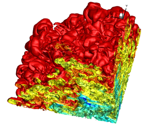
First of all, the isosurfaces of mass fractions of SF6 for spherical and cylindrical converging RMI at different moments are displayed in figures 4 and 5, respectively. In order to observe the degree of mixing between species, only one eighth of the main computational domain is shown for each isosurface. As we can see from these isosurfaces, the evolution processes of the amplitudes of perturbations for spherical and cylindrical converging RMI are basically identical. Firstly, the phase inversion phenomenon is observed as the shock wave converges from the heavy fluid into the light fluid. The amplitudes of the perturbations decrease after the shock waves first pass through the interfaces from the heavy fluids, so that the isosurfaces are smoother at  $t = 0.01\;\textrm{ms}$. Then, the reflected shock waves interact with the interfaces secondly, resulting in abundant large-scale bubble structures being generated on the interfaces (see the isosurfaces at
  $t = 0.02\;\textrm{ms}$ and
  $0.04\;\textrm{ms}$). Finally, these large-scale bubbles interact with each other and break into a large number of small-scale structures, and the turbulent mixing begins (see the isosurfaces at
  $t = 0.08\;\textrm{ms}$ and
  $0.2\;\textrm{ms}$).

Figure 4. Isosurfaces of mass fraction of SF6 for spherical converging RMI at  $t = 0\;\textrm{ms}$,
  $0.01\;\textrm{ms}$,
  $0.02\;\textrm{ms}$,
  $0.04\;\textrm{ms}$,
  $0.08\;\textrm{ms}$ and
  $0.2\;\textrm{ms}$. Only one eighth of the main computational domain is shown for each isosurface.

Figure 5. Isosurfaces of mass fraction of SF6 for cylindrical converging RMI at  $t = 0\;\textrm{ms}$,
  $0.01\;\textrm{ms}$,
  $0.02\;\textrm{ms}$,
  $0.04\;\textrm{ms}$,
  $0.08\;\textrm{ms}$ and
  $0.2\;\textrm{ms}$. Only one eighth of the main computational domain is shown for each isosurface.
The shock wave is the main driving force and energy source of RMI. Therefore, it is of great physical significance to correctly capture the trajectory of the shock wave. Figure 6 shows the wave diagram illustrating the main shock wave positions,  ${r_s}$, and the outer radii of the mixing layers for spherical and cylindrical converging RMI. The shock wave positions are identified by the absolute maximum of velocity divergence, i.e.
  $\max (|\boldsymbol{\nabla }\boldsymbol{\cdot }V|)$. As shown in figure 6, before the converging shock waves pass through the interfaces for the first time, i.e.
  $t < 0.005\;\textrm{ms}$, the velocities of the spherical and cylindrical converging shock waves are identical. After the shock waves are incident into light fluids from heavy fluids, the velocities of the shock waves increase obviously due to the changes of specific heat ratios, and the velocity of the spherical converging shock wave is faster than that of the cylindrical converging shock wave. The spherical transmitted shock wave arrives at the converging centre point at
  $t = 0.019\;\textrm{ms}$. The cylindrical transmitted shock wave arrives at the converging centre line at
  $t = 0.021\;\textrm{ms}$. Transmitted shock waves are reflected at the converging centres and transformed into reflected shock waves. After reflections, the difference of velocity difference between spherical and cylindrical reflected shock waves is further enlarged. The spherical reflected shock wave interacts with the interface at
  $t = 0.026\;\textrm{ms}$, and the cylindrical reflected shock wave passes through the interface at
  $t = 0.03\;\textrm{ms}$. Due to the decreases of specific heat ratios, the velocities of the reflected shock waves become slower after they are transmitted from light fluids into heavy fluids. In a word, the geometric effect (sphere or cylinder) has a great impact on the trajectory of the shock wave.

Figure 6. Wave diagram showing main shock wave positions and the outer radii of the mixing layers.
The mixing layer width of RMI is one of the most important physical quantities in practical engineering applications. Studies on the planar RMI show that the increase of the turbulent mixing layer width follows the law of  $h\sim {t^\theta }$. However, different studies have given different exponents
  $\theta $.
The time evolutions of the mixing layer widths for spherical and cylindrical converging RMI are shown in figure 7. The mixing layer width h are defined as
 \begin{equation}h = {r_2} - {r_1}.\end{equation}
It can be seen from figure 7 that, after the shock waves interact with interfaces for the first time, the initial mixing layer widths are compressed and reduce to the minimum values. From here until  $t = 0.026\;\textrm{ms}$ for the spherical mixing layer and
  $t = 0.03\;\textrm{ms}$ for the cylindrical mixing layer, the heavy fluids accelerate the light fluids in the mixing layers, so the flow is RT stable. The RT stable effect results in a weak or even negative growth of the mixing layer width. After the reflected shock waves impact interfaces again, the light fluids accelerate the heavy fluids in the mixing layers, and the flow is RT unstable. The mixing layer widths begin to grow rapidly, first linearly, then nonlinearly and finally reach the asymptotic saturation levels. In the linear growth stage, for spherical converging RMI, the mixing layer width varies as
  $h\sim 0.7t{U_r}$. For the cylindrical converging RMI, the mixing layer width varies as
  $h\sim 0.58t{U_r}$, which indicates that the linear growth rate of the cylindrical mixing layer is approximately 17 % lower than that of the spherical mixing layer. The asymptotic values of spherical and cylindrical mixing layer widths are
  $5.1\;\textrm{mm}(0.73{R_0}\textrm{)}$ and
  $4.6\;\textrm{mm}(0.66{R_0})$, respectively. There is a difference of approximately 10 % between the asymptotic values of spherical and cylindrical mixing layer widths. On the whole, the geometric effect has a great influence on the developments of the mixing layer widths, and the width of spherical mixing layer is obviously larger than that of the cylindrical mixing layer. The main reason for this phenomenon may be that the spherical mixing layer converges toward the centre point from three directions, while the cylindrical mixing layer converges toward the centre line from only two directions, so that the BP effect of spherical converging geometric is stronger.

Figure 7. The width of the mixing layer vs. time. Here,  ${t_1}$ is the moment when the shock waves first hit the interfaces;
  ${t_2}$ and
  ${t_3}$ are the moments when the spherical and cylindrical reflected shock waves hit the interfaces for the second time, respectively.
According to the inner and outer radii of the mixing layer, the heights of the bubble (light fluid penetrates heavy fluid) and spike (heavy fluid penetrates light fluid) can be defined as,
 \begin{equation}{h_b} = {r_2} - {r_{0.5}},\quad {h_s} = {r_1} - {r_{0.5}}.\end{equation}
Here, the  ${r_{0.5}}$ denotes the position where the mass fractions of light and heavy fluids both are
  $0.5$. It can be clearly seen from figure 8 that, for the cylindrical converging RMI, the bubble height always increases linearly and gently. For the spherical converging RMI, the bubble height has a rapid growth stage (approximately in the range
  $0.05\;\textrm{ms} < t < 0.07\;\textrm{ms}$). This is mainly because the spherical mixing layer has a geometric divergence effect outwards. However, as large-scale bubbles interfere with each other and break into small-scale structures, the mixing layer enters the turbulent mixing stage, and the spherical geometrical outward divergence effect no longer plays a dominant role. Then, the bubble height of spherical mixing layer also enters a slow linear growth stage. For spherical and cylindrical converging RMI, the spikes reach the centre at approximately 0.1 ms, and from then on the spike positions remains constant.

Figure 8. The heights of the bubble and spike vs. time.
Figure 9 displays the time developments of mass fractions of SF6 in the mixing layers. The distribution of mass fraction can, to a certain extent, characterize the mixing degree of the two fluids, which includes not only the mixing at the molecular level, but also the mixing of pure light/heavy fluid entering into heavy/light fluid through the bubble/spike structures and still maintaining the pure fluid state. As shown in figure 9, before the reflected shock waves pass through mixing layers, the mass fractions of SF6 in the spherical and cylindrical mixing layers are roughly the same. The main reason is that the first interactions between converging shock waves and interfaces cause the amplitudes of interfacial perturbations to decrease. Meanwhile, the bubble and spike structures are relatively small and develop slowly, and the influences of the geometric effect are insignificant. In addition, as the shock waves converge from the heavy fluids into the light fluids, so-called phase inversion phenomena occur, that is, the amplitudes of the initial perturbations on the interfaces first decrease and then increase in reverse. In other words, the light and heavy fluids first separate from each other, and then penetrate each other, which is also the reasons that the mass fraction of SF6 fluctuates during this stage. After the second interactions between reflected shock waves and interfaces, the widths of the spherical and cylindrical mixing layers start to grow quickly and the bubble and spike structures develop rapidly so that a large amount of pure fluids are brought into the other pure fluids. During this stage, the geometric effect becomes very important, resulting in a large difference in the mass fractions of SF6 in spherical and cylindrical mixing layers, and the mass fraction of SF6 in the spherical mixing layer is significantly higher than that in the cylindrical mixing layer. This means that the spherical mixing layer brings more SF6 from the periphery into the mixing layer. For spherical and cylindrical mixing layers, the light fluid is completely mixed after approximately 0.1 ms. Thus, the mass of light fluids in the mixing layer remains constant and only the mass of heavy fluids increases. This is also why the mass fractions of SF6 are large at the end of the two numerical simulations.

Figure 9. Mass fraction of SF6 in the mixing layer vs. time.
For viscous flow, physical viscosity can dissipate the small-scale structures and convert kinetic energy into internal energy. The Taylor microscale is the length scale at which viscosity begins to have a significant effect on the flow. Here, the radial Taylor microscale  $\lambda $ is defined as,
 \begin{equation}{\lambda ^2} = \frac{{\langle u^{\prime\prime^2}_r\rangle }}{{\langle {{(\partial {{u^{\prime\prime}}_r}/\partial r)}^2}\rangle }}.\end{equation}
The Taylor Reynolds number  $R{e_\lambda }$ based on the Taylor microscale and Reynolds number
  $R{e_h}$ based on the mixing layer width can be defined as, respectively,
 \begin{equation}R{e_\lambda } = \frac{{{u_{rms}}\lambda }}{\nu },\quad R{e_h} = \frac{{{u_{rms}}h}}{\nu }.\end{equation}
Here,  ${u_{rms}}( = \sqrt {\langle u^{\prime\prime^2}_r\rangle } )$ and
  $\nu ( = \mu /\rho )$ are the root mean square of the radial velocity and the kinematic viscosity in the entire mixing layer, respectively. As shown in figure 10(a), the maximum peak values of the time evolutions of the radial Taylor microscales in the spherical and cylindrical mixing layers both are approximately 0.1 mm
  $({\approx} 0.014{R_0})$. Combined with figure 7, it can be found that the radial Taylor microscales basically tend to remain unchanged after the end of the linear growth stages of the mixing layer widths. The asymptotic values of the radial Taylor microscales for spherical and cylindrical mixing layers are approximately 0.08 mm
  $({\approx} 0.011{R_0})$ and 0.095 mm
  $({\approx} 0.014{R_0})$ respectively. In addition, it is important to note that the radial Taylor microscale is very dependent on the mesh resolution. Figure 10(b) describes the time developments of the Taylor Reynolds numbers. The maximum peak value of the Taylor Reynolds number in the spherical mixing layer is approximately 2000. However, the maximum peak value of the Taylor Reynolds number in the cylindrical mixing layer is only approximately 1000, which only is half of that in the spherical mixing layer. In the late stage, the Taylor Reynolds numbers in the spherical and cylindrical mixing layers gradually decay to the same value. The time development of the Reynolds numbers based on the mixing layer width is shown in figure 10(c). The peak value of
  $R{e_h}$ for the spherical mixing layer is approximately 48 000. However, it is only approximately 31 000 for the cylindrical mixing layer.

Figure 10. Radial Taylor microscale (a), Taylor Reynolds number (b) and Reynolds number based on mixing layer width (c) vs. time.
The helicity  ${h_t}$ is also a noteworthy quantity, and is defined as,
 \begin{equation}{h_t} = {u_i}{\omega _i},\end{equation}
where  ${\omega _i}$ denotes the velocity curl. The helicity is a quadratic invariant in addition to the kinetic energy of the three-dimensional NS equations in the inviscid limit. Yu et al. (Reference Yu, Hong, Xiao and Chen2013) proposed a LES model by considering the inertial range balance of subgrid-scale helicity dissipation in physical and spectral spaces and the joint cascade of energy and helicity. Therefore, the studies on the evolution mechanisms of helicity in the turbulent mixing layer induced by RMI are helpful to establish a new model or improve the existing model for the turbulent mixing problem. The time developments of helicity in the mixing layers are displayed in figure 11. After the reflected shock waves hit the interfaces for the second time, the helicity begins to increase rapidly. On the whole, compared with the cylindrical mixing layer, the spherical mixing layer has higher helicity. The peak of helicity appears at approximately
  $t = 0.055\;\textrm{ms}$. The radial distribution of helicity at
  $t = 0.055\;\textrm{ms}$ is shown in figure 12(a). It can be found that, at this moment, the helicity in the spherical and cylindrical mixing layers has a regular and similar chirality. Due to the effect of viscous dissipation, the average helicities both tend to be zero at the later stage of spherical and cylindrical mixing layers. The radial distribution of helicity at
  $t = 0.2\;\textrm{ms}$ is shown in figure 12(b). At this moment, the helicity in the mixing layer has no regular chirality and shows the characteristic of fluctuating up and down around zero.

Figure 11. Helicity in the mixing layer vs. time.

Figure 12. Radial distribution of helicity at  $t = 0.055\;\textrm{ms}$ (a) and
  $t = 0.2\;\textrm{ms}$ (b).
The time evolutions of the root mean square of the velocities and turbulent kinetic energy (TKE) in the mixing layers are shown in figure 13. Here, the turbulent kinetic energy is defined as,
 \begin{equation}TKE = {\textstyle{1 \over 2}}\langle \rho {u^{\prime\prime}_i}{u^{\prime\prime}_i}\rangle /\langle \rho \rangle .\end{equation}
As shown in figure 13, for both the spherical mixing layer and the cylindrical mixing layer, the time development trend of TKE is very similar to that of the root mean square of the velocities. The difference is that the root mean square of the velocities and the TKE in the spherical mixing layer exhibit a single peak characteristic. However, they show a three-peak characteristic in the cylindrical mixing layer, although the third peak may be less obvious. The reason for this difference may be that different geometries have different reflection or transmission effects on shock waves. At the later stage, the root mean square of the velocities in the cylindrical mixing layer are at least approximately 50 % larger than that in the spherical mixing layer, which indicates that the turbulent intensity in the cylindrical mixing layer is higher. In terms of TKE, after  $t > 0.1\;\textrm{ms}$, at this time when the spherical and cylindrical mixing layer widths begin to reach asymptotic saturation, the TKEs have a power-law decay with time, i.e.
  $TKE\sim {t^{ - n}}$. Groom & Thornber (Reference Groom and Thornber2021) find that the decay rate n of TKE is 1.51–2.20 in planar RMI, and the decay rate decreases with increasing initial Reynolds number. In the present numerical simulations, the decay exponents of the TKE in spherical and cylindrical mixing layers both are n = 2.20. This indicates that the turbulent mixing effect is more dominant than the geometric effect in the turbulent mixing stage.

Figure 13. Root mean square of velocities (a–c) and turbulent kinetic energy (d) in the mixing layer vs. time. For spherical converging RMI, u is the radial velocity, v is velocity in the  $\varphi (0 \le \varphi \le 2{\rm \pi} )$ direction, w is the velocity in the
  $\theta (0 \le \varphi \le {\rm \pi})$ direction. For cylindrical converging RMI, u is the radial velocity, v is the velocity in the
  $\varphi (0 \le \varphi \le 2{\rm \pi} )$ direction, w is the velocity in the z direction.
As mentioned above, the RMI is mainly caused by the baroclinic vorticity. Therefore, the analysis of the physical quantities related to the vortex dynamics can deepen our understanding of the intrinsic mechanism of RMI. In our previous paper (Fu et al. Reference Fu, Yu and Li2020), the enstrophy transport equation has been analysed in detail. The enstrophy is defined as,
 \begin{equation}\varOmega = {\textstyle{1 \over 2}}{\omega _i}{\omega _i}.\end{equation}
Figure 14 shows the time evolutions of the enstrophy in the spherical and cylindrical mixing layers. From figure 14(a,b), it can be found that, for both spherical and cylindrical converging RMI, refining the mesh greatly increases the enstrophy, which is similar to the numerical results of Hahn et al. (Reference Hahn, Drikakis, Youngs and Williams2011). In addition, we also find that the quantities that do not include the partial derivatives of the velocities have reached mesh convergence, while the quantities that include the partial derivatives of the velocities, such as the dissipation rate, enstrophy and Taylor scale, have not reached mesh convergence. This is a consequence of using the ILES approach which resolves more and more of the fine-scale structure as the mesh is refined. The peak value of enstrophy in the spherical mixing layer is much larger than that in the cylindrical mixing layer. Combined with figure 7, it can be found that the time interval corresponding to the linear growth stage of mixing layers is approximately  $0.03\;\textrm{ms} < t < 0.08\;\textrm{ms}$, which is exactly consistent with the peak interval of enstrophy. And outside of this time interval, the enstrophy tends to be zero. Therefore, it can be concluded that the developments of enstrophy are closely related to the increases of the mixing layer widths, and larger enstrophy is more conducive to the growth of the mixing layer widths. When the spherical and cylindrical mixing layer widths begin to reach asymptotic saturation (approximately
  $t > 0.1\;\textrm{ms}$), the enstrophy has a power-law decay with time, i.e.
  $\varOmega \sim {t^{ - a}}$. In the spherical mixing layer, the decay exponents of enstrophy is a = 2.58. In the cylindrical mixing layer, the decay exponents of enstrophy is a = 2.42. The geometric effect has little effect on the decay exponent of enstrophy.

Figure 14. Enstrophy in the mixing layer vs. time.
The probability density functions (PDF) of the mass fractions of SF6 in the spherical and cylindrical mixing layers at  $t = 0.2\;\textrm{ms}$ are displayed in figure 15. It can be found that the PDF of the mass fractions of SF6 in spherical and cylindrical mixing layers have bimodal characteristics. The first peak value of the PDF appears at the position of
  ${Y_{\textrm{SF6}}} = 0.89$ in the spherical mixing layer, and at the position of
  ${Y_{\textrm{SF6}}} = 0.8$ in the cylindrical mixing layer. The second peak values of the PDF appear at the positions of
  ${Y_{\textrm{SF6}}} = 1$, which indicates that there is still a large amount of pure SF6 in the mixing layers. In the range of low mass fraction, the PDF in the cylindrical mixing layer is larger, and the left tail is flatter, which shows that the mixing degree between light and heavy fluids in the spherical mixing layer is greater than that in the cylindrical mixing layer.

Figure 15. Probability density function of the mass fraction of SF6 in the mixing layer at  $t = 0.2\;\textrm{ms}$.
Figure 16 describes the time developments of the skewness and kurtosis factors in the spherical and cylindrical mixing layers. The skewness and kurtosis factors can be used to describe the degree of deviation of the radial fluctuation velocity from the Gaussian distribution due to the existence of turbulent intermittency. If a random variable of zero mean is Gaussian, then its skewness factor S would be equal to 0 and kurtosis factor K would be equal to 3. In addition, the skewness factor can also characterize the rate at which the enstrophy increase by vortex stretching, and the equation is  $s = (135/98)^{1/2}\langle {\omega _i}{\omega _j}(\partial {u_i}/\partial {x_j})\rangle /{\varOmega ^{3/2}}$ (Lesieur Reference Lesieur1997). Figure 16 shows that at the later turbulent mixing stage, both the skewness and kurtosis factors of the radial fluctuation velocity in the cylindrical mixing layer are larger, indicating stronger turbulent intermittency.

Figure 16. Skewness (a) and kurtosis factors (b) in the mixing layer vs. time.
The mixing layer width and mass fraction distribution can, to some extent, characterize the mixing degree of different fluids, but, as mentioned above, these two quantities cannot distinguish whether the mixing is true molecular-level mixing. There are many parameters that have been proposed to measure the molecular mixing degree. Zhou et al. (Reference Zhou, Cabot and Thornber2016) compared in detail the asymptotic behaviour of different mixing parameters in plane RTI and RMI with different density ratios. In this paper, the molecular mixing fraction  $\theta $ defined by Youngs (Reference Youngs1991, Reference Youngs1994) is used to measure the molecular mixing degree
 \begin{equation}\mathrm{\theta } = \frac{{\int {{X_1}{X_2}\,\textrm{d}V} }}{{\int {\langle {X_1}\rangle \langle {X_2}\rangle \,\textrm{d}V} }}.\end{equation}
Here,  $\theta = 1$ denotes perfect mixing and
  $\theta = 0$ denotes complete separation;
  ${X_k}$ denotes the volume fraction of species k. The time developments of the molecular mixing fractions of the spherical and cylindrical mixing layers are shown in figure 17. The molecular mixing fractions of spherical and cylindrical mixing layers first decrease monotonically and then increase monotonically. This is because, at the early stage, the mixing layer is mainly composed of pure fluids that penetrate each other. The molecular mixing fraction decreases with the increase of the bubble and spike structures. After the reflected shock, the pure fluid begins to break up into small structures and molecular mixing causes the molecular mixing fraction to increase again. At the later stage, the increases of molecular mixing fractions slow down and begin to reach the asymptotic values. At the growth stage, the molecular mixing fraction in the spherical mixing layer is always larger. In other words, the fluid in spherical mixing layer is more fully mixed. In addition, comparing figure 17 with figure 14, it can be found that the time interval corresponding to the fastest growth rates of molecular mixing fractions is basically consistent with the peak interval of enstrophy and linear growth interval of the mixing layer width. This is mainly because the magnitudes of enstrophy can represent the strength of vorticity, and the rotational motions of the vortex can accelerate the mixing between light and heavy fluids.

Figure 17. Molecular mixing fraction vs. time.
The efficiency Atwood number can be defined as,
 \begin{equation}{A_e} = \frac{{{\rho _{rms}}}}{{\langle \rho \rangle }}.\end{equation}
The efficiency Atwood number is a quantity related to the turbulent mixing and mixing layer width growth. As  ${A_e}$ decreases, the entrainment, which is responsible for bringing the large pockets of irrotational fluid into the turbulent flow region, is weakened gradually and the turbulent mixing is strengthened gradually. Conversely, when
  ${A_e}$ increases, pure fluids come into the turbulent flow region faster than they are mixed. Cook, Cabot & Miller (Reference Cook, Cabot and Miller2004) believe that, at the stage of mixing transition, the turbulent mixing rate overtakes the entrainment rate so that the growth rate of the mixing layer width is reduced. As shown in figure 18, the time evolution trends of the efficiency Atwood numbers in the spherical and cylindrical mixing layers are the inverse of the molecular mixing fractions. This reason is that the efficiency Atwood number increases monotonically, indicating that the turbulent mixing rate is weakening compared with the entrainment rate, so the molecular mixing fraction decreases monotonically. Conversely, the efficiency Atwood number decreases monotonically, indicating that the turbulent mixing is being intensified, so the molecular mixing fraction increases monotonically. At the later stage, the efficiency Atwood number in the spherical mixing layer is always smaller, indicating that the turbulent mixing rate is faster in the spherical mixing layer.

Figure 18. Efficiency Atwood number in the mixing layer vs. time.
The turbulent mass-flux velocity  ${a_i} ={-} \langle u^{\prime\prime}\rangle $ is also an important source term related to turbulent mixing. For the three-equation Reynolds-averaged Navier–Stokes model, i.e.
  $k {-} L {-} a$ mode (Morgan & Wickett Reference Morgan and Wickett2015), the turbulent mass-flux velocity as a prefactor appears in the energy equation, TKE equation and turbulent mass-flux velocity equation. Therefore, the study of the turbulent mass-flux velocity is beneficial to improve the turbulent mixing model. Mohaghar et al. (Reference Mohaghar, Carter, Musci, Reilly, Mcfarland and Ranjan2017) and Reese et al. (Reference Reese, Ames, Noble, Oakley, Rathamer and Bonazza2018) use the density-weighted turbulent mass-flux velocity
  ${a_i} = \langle \rho ^{\prime}{u^{\prime}_i}\rangle /\langle \rho \rangle$ in their papers instead of
  $- \langle u^{\prime\prime}\rangle $. However, it can be proved that these two are equal, i.e.
 \begin{equation}{a_i} ={-} \langle u^{\prime\prime}\rangle = \left\langle {\frac{{\langle \rho u\rangle }}{{\langle \rho \rangle }} - \frac{{\langle \rho \rangle u}}{{\langle \rho \rangle }}} \right\rangle = \left\langle {\frac{{\langle \rho \rangle \langle u\rangle + \langle \rho^{\prime}u^{\prime}\rangle - \langle \rho \rangle \langle u\rangle - \langle \rho \rangle u^{\prime}}}{{\langle \rho \rangle }}} \right\rangle = \frac{{\langle \rho ^{\prime}u^{\prime}\rangle }}{{\langle \rho \rangle }}.\end{equation}
The radial distributions of turbulent mass-flux velocities at  $t = 0.2\;\textrm{ms}$ for spherical and cylindrical mixing layers are shown in figure 19(a). The radial distance is normalized by the inner and outer radii of mixing layer. First, it can be found that the turbulent masses are transported mainly in the radial directions. In addition, the radial turbulent mass-flux velocities
  ${a_1}$ in the mixing layers are all negative. However,
  ${a_1}$ being predominantly negative does not indicate net negative fluctuation, or the transport of turbulence and mass inwards. It indicates that, in a spherical or cylindrical averaging shell (as shown in figure 19b), the negative mass fluctuations are paired with positive radial velocity fluctuations, and positive mass fluctuations are correlated with negative radial velocity fluctuations. In other words, the light fluids are being transported from the centre outward, and the heavy fluids are being transported from the periphery inward. This leads to mutual penetration and turbulent mixing between the two fluids. The larger the turbulent mass-flux velocity is, the more intense the turbulent mass exchange is. At the later stage, because the species in the spherical mixing layer have been mixed more fully, the turbulent mass-flux velocity is generally smaller than that in the cylindrical mixing layer. The values of
  ${a_2}$ and
  ${a_3}$ both are close to zero, which means that the mass and velocity fluctuations are uncorrelated, without a preferential direction of transport over the whole radial spherical or cylindrical shell.

Figure 19. (a) Radial distribution of turbulent mass-flux velocity at  $t = 0.2\;\textrm{ms}$. (b) schematic of radial turbulent mass-flux velocity.
The density self-correlation b can also be used to measure the fluid mixing and is defined as,
 \begin{equation}b ={-} \left\langle {\rho^{\prime}{{\left( {\frac{1}{\rho }} \right)}^\prime }} \right\rangle .\end{equation}
Here,  $b = 0$ indicates that the fluid is perfect mixed fluid or pure fluid. The density self-correlation as a prefactor appears in the production term of the turbulent mass-flux velocity equation in the
  $k - L - a$ model and is closed by a algebraic equation, i.e.
 \begin{equation}b = \bar{\rho }\left( {\frac{{\sum\limits_k {\frac{{{X_k}}}{{{\rho_k} + c\bar{\rho }}}} }}{{\sum\limits_k {\frac{{{X_k}{\rho_k}}}{{{\rho_k} + c\bar{\rho }}}} }}} \right) - 1.\end{equation}
Here, c is an undetermined model constant and is set as zero through similarity analysis. The radial distributions of the density self-correlations calculated by using (3.11) and (3.12) for spherical and cylindrical mixing layers at  $t = 0.2\;\textrm{ms}$ are shown in figure 20. For convenience of viewing, the results of (3.12) are multiplied by the corresponding coefficients to ensure that the peak values of the density self-correlations are equal. In terms of the results of (3.11), outside the mixing layers, because the fluids are pure heavy fluids, the density self-correlations are both zero for spherical and cylindrical mixing layers. In the mixing layers, the density self-correlation of the spherical mixing layer is generally lower than that of the cylindrical mixing layer, which again indicates that there are more unmixed pure fluid bubbles in the cylindrical mixing layer. Comparing the results of (3.11) with (3.12) in figure 20, it can be found that the density self-correlations calculated using the algebraic equation of the
  $k {-} L {-} a$ model are different in magnitude. In addition, the shapes of the radial distribution of the real results and algebraic equation results are also very different, especially for the spherical converging geometry. The main reason for this phenomenon may be that the model constant c in the
  $k {-} L {-} a$ model is obtained by self-similarity analysis of one-dimensional RTI and RMI in the low Atwood number limit, and the influence of the geometric effect is also not considered. Therefore, it is necessary to improve this algebraic equation.


The Reynolds stresses are one of the most important unclosed terms in Reynolds-averaged Navier–Stokes model, which are defined as,
 \begin{equation}{R_{ij}} = \langle \rho {u^{\prime\prime}_i}{u^{\prime\prime}_j}\rangle .\end{equation}
Figure 21(a) describes the radial distributions of Reynolds stresses in spherical and cylindrical mixing layers at  $t = 0.2\;\textrm{ms}$. Compared with the Reynolds normal stresses
  $({R_{11}},{R_{22}},{R_{33}})$, the Reynolds shear stresses
  $({R_{12}},{R_{13}},{R_{23}})$ are negligible, which indicates that the shear effects in the mixing layers are very small and the turbulent production is of baroclinic type. According to the Reynolds stresses, the Reynolds stress anisotropy tensor can be defined as,
 \begin{equation}{b_{ij}} = \frac{{\langle \rho {{u^{\prime\prime}}_i}{{u^{\prime\prime}}_j}\rangle }}{{\langle \rho {{u^{\prime\prime}}_k}{{u^{\prime\prime}}_k}\rangle }} - \frac{1}{3}{\delta _{ij}}.\end{equation}
The value of  ${b_{ij}}$ is between
  $- 1/3$ and
  $2/3$. If
  ${b_{ij}} ={-} 1/3$, that means there is no TKE distributed in this direction, and if
  ${b_{ij}} = 2/3$, that means that all the TKE is occupied in this direction. The time developments of the Reynolds stress anisotropy tensors in the spherical and cylindrical mixing layers are displayed in figure 21(b). When the reflected shock waves pass through the interfaces for the second time, the Reynolds stress anisotropy in spherical and cylindrical mixing layers reaches its peak value. The peak values are 0.48 and 0.42 for the spherical and cylindrical mixing layers, respectively. This means that approximately 81 % of TKE is in the radial direction for the spherical mixing layer, and approximately 75 % of TKE is in the radial direction for the cylindrical mixing layer. Then, with the increase of time, the anisotropy decreases monotonically, indicating that the flows in the mixing layers are developing toward isotropy. Finally,
  ${b_{11}}$ in the spherical mixing layer tends to 0.07, that is, approximately 40 % of TKE is distributed in the radial direction. The value of
  ${b_{11}}$ in the cylindrical mixing layer tends to 0.09, that is, approximately 42 % of TKE is distributed in the radial direction. The spherical mixing layer is more isotropic.

Figure 21. (a) Radial distribution of Reynolds stress at  $t = 0.2\;\textrm{ms}$. (b) Anisotropy of Reynolds stress in the mixing layer vs. time.
Next, the method of conditional statistics will be applied in the mixing layers to study the influence of the geometric effect under given conditions. Here, conditional statistics means that, at a certain moment, within a certain space range, the data on the grid points satisfying the given condition are recombined into a new data set, and then statistical analysis is carried out on this new data set. The mass fraction is an extremely important physical quantity in the turbulent mixing induced by the interfacial instability. Therefore, in the present paper, the mass fraction of SF6 is selected as the condition to perform conditional statistics.
Figure 22 shows the conditional mean of the radial velocity in mass fraction space in the spherical and cylindrical mixing layers at  $t = 0.2\;\textrm{ms}$. It can be seen from figure 22 that the radial velocities are obviously dependent on the mass fractions. For the spherical mixing layer, when
  ${Y_{\textrm{SF6}}} < 0.89$, the conditional mean of the radial velocity is greater than zero. When
  ${Y_{\textrm{SF6}}} > 0.89$, the conditional mean of the radial velocity is smaller than zero. For the cylindrical mixing layer, when
  ${Y_{\textrm{SF6}}} < 0.82$, the conditional mean of the radial velocity is greater than zero. When
  ${Y_{\textrm{SF6}}} > 0.82$, the conditional mean of the radial velocity is smaller than zero. Combined with figure 15, it can be found that values of 0.89 and 0.82 roughly correspond to the peak values of the PDF of the mass fraction of SF6 in spherical and cylindrical mixing layers. This is mainly because the mixing degree between heavy and light fluids tends to the peak position of the PDF. Therefore, a fluid element that is less mixed than the peak position of PDF moves outward and mixes with the SF6 fluid. A fluid element with a mixing degree greater than the peak position of PDF moves inward and mixes with the N2 fluid. Figure 23 shows the conditional root mean square of the radial velocity in mass fraction space in the spherical and cylindrical mixing layers at
  $t = 0.2\;\textrm{ms}$. Obviously, in the whole mass fraction space, the conditional root mean square of the radial velocity in the cylindrical mixing layer is always larger. Therefore, it can be concluded that in the mass fraction space, the turbulent intensity is stronger in the cylindrical mixing layer.

Figure 22. Conditional mean of the radial velocity in mass fraction space in the mixing layer at  $t = 0.2\;\textrm{ms}$.

Figure 23. Conditional root mean square of the radial velocity in mass fraction space in the mixing layer at  $t = 0.2\;\textrm{ms}$.
Figure 24 shows the conditional mean of the velocity divergence in mass fraction space in the spherical and cylindrical mixing layers at  $t = 0.2\;\textrm{ms}$. The velocity divergence can be used to measure the compression and expansion effects of the fluids. If the velocity divergences are greater than zero, the fluids are expanding. Conversely, if the velocity divergences are smaller than zero, the fluids are being compressed. We see from figure 24 that the velocity divergence is also dependent on the mass fraction. In addition, it can be found that a fluid element with a mixing degree smaller than the peak position of the PDF of the mass fraction of SF6 is compressed, and a fluid element with a mixing degree greater than the peak position of the PDF of the mass fraction of SF6 is expanding.

Figure 24. Conditional mean of the velocity divergence in mass fraction space in the mixing layer at  $t = 0.2\;\textrm{ms}$.
Figure 25 shows the conditional mean of enstrophy in mass fraction space in the spherical and cylindrical mixing layers at  $t = 0.2\;\textrm{ms}$. The enstrophy has a significant dependence on the mass fractions, and the geometric effect has a great influence on the conditional mean of enstrophy.

Figure 25. Conditional mean of enstrophy in mass fraction space in the mixing layer at  $t = 0.2\;\textrm{ms}$.
4. Conclusions
In this paper, comprehensive analysis is conducted for the high resolution ILES data of spherical and cylindrical converging RMI with a grid size of 20483. The numerical results show that,
(i) The linear growth rate of spherical mixing layer is faster than that of cylindrical mixing layer. The degree of mixing in the spherical mixing layer is greater. The turbulence in the cylindrical mixing layer is more intermittent.
(ii) Because of the geometric divergence effect outward, the bubble height has a rapid growth stage in the spherical mixing layer.
(iii) At the early stage, the helicity in the spherical and cylindrical mixing layers has a regular and similar chirality. Compared with the Reynolds normal stresses, the Reynolds shear stresses in the spherical and cylindrical mixing layers are negligible. There is strong anisotropy in the mixing layers at the early stage, but the mixing layers tend to become gradually isotropic as the developments of time. At the later stage, the TKE and enstrophy have a power-law decay with time, and the geometric effect has little effect on the decay exponent.
(iv) The conditional statistics analysis shows that the radial velocities, root mean square of the radial velocity, velocity divergence and enstrophy in the spherical and cylindrical mixing layers are obviously dependent on the mass fractions. In the mass fraction space, the turbulent intensity is stronger in the cylindrical mixing layer.
Funding
This work was supported by the National Key Research and Development Program of China (Grant Nos 2019YFA0405300, 2016YFA0401200), NSFC Projects (Grant Nos 91852203, 12072349.), the Science Challenge Project (Grant No. TZ2016001) and National Numerical Wind Tunnel Project. The authors thank the National Supercomputer Center in Tianjin (NSCC-TJ) and the National Supercomputer Center in Guangzhou (NSCC-GZ) for providing computer time.
Declaration of interests
The authors report no conflict of interest.
Appendix A.
In this paper, we use the polynomial fit of the logarithm of the viscosity and thermal conductivity coefficients versus the logarithm of the temperature to obtain the transport properties of species k. The coefficients of the polynomial fit can be found in tables 2 and 3.
Table 2. The coefficients of polynomial fit for the viscosity of species k. The unit of the viscosity coefficient computed by using (2.7) is  $\textrm{g}\;{(\textrm{cm}\ \textrm{s})^{ - 1}}$.

Table 3. The coefficients of polynomial fit for the thermal conductivity of species k. The unit of the thermal conductivity coefficient computed by using (2.8) is  $\textrm{erg}\;{(\textrm{cm}\ \textrm{s}\ \textrm{K})^{ - 1}}$.


