


As political scientists increasingly focus on the identification of causal effects, instrumental variable (IV) models are becoming commonplace (e.g., Sovey and Green, Reference Sovey and Green2011). IV models hinge on the validity of the instrument. While researchers are usually aware of conditional independence and relevance as general requirements for valid instruments, we identify a specific threat that is frequently ignored: spatial interdependence in the outcome variable. Our review of IV models in leading political science journals reveals that authors rarely discuss and never empirically address spatial interdependence as a threat to inference (see Figure 1), even as theories of spatial interdependence and diffusion proliferate across political science (see, e.g., Siverson and Starr Reference Siverson and Starr1990; Starr Reference Starr1991; Ward and Gleditsch Reference Ward and Gleditsch2002; Ward and O’Loughlin Reference Ward and O’Loughlin2002; Simmons, Dobbin and Garrett Reference Simmons, Dobbin and Garrett2006; Franzese and Hays Reference Franzese and Hays2007; Plümper and Neumayer Reference Plümper and Neumayer2010).Footnote 1
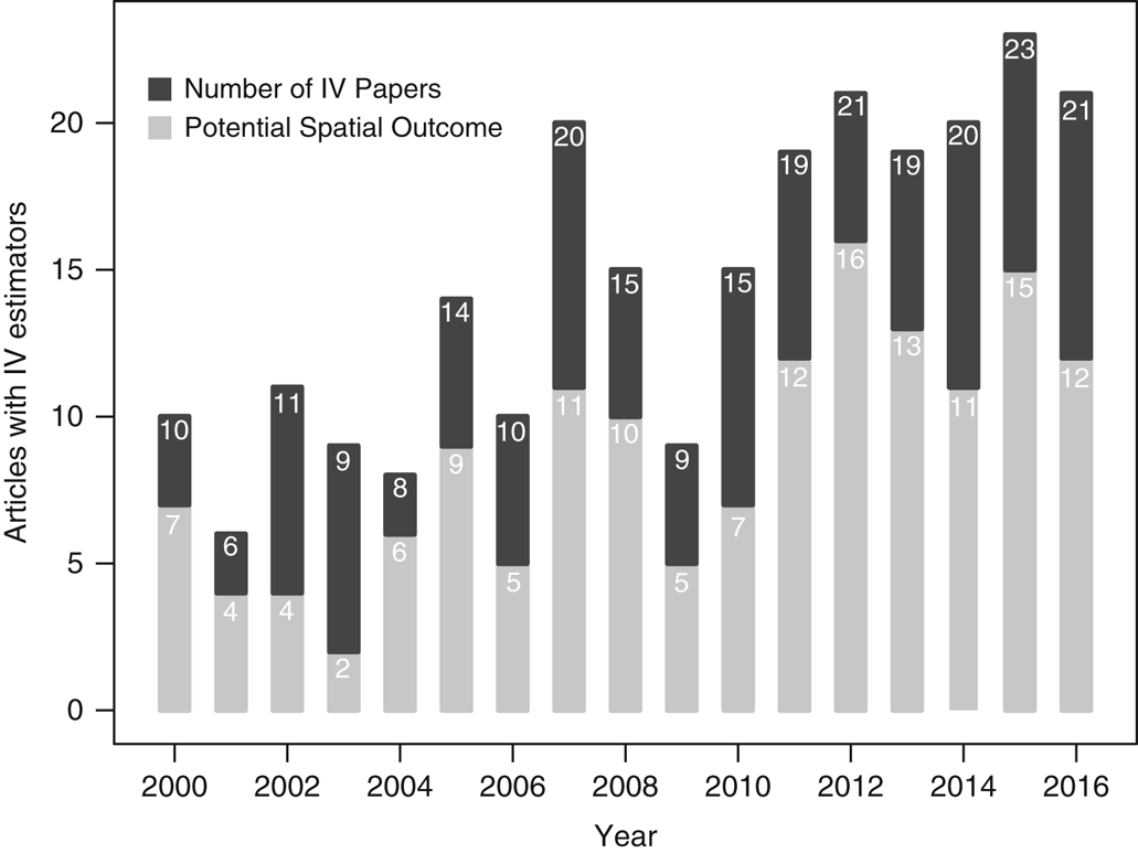
Figure 1 The plot shows the number of articles published in the APSR, AJPS, JOP, IO, BJPS, and World Politics between 2000 and 2016 that use IV models (light gray bars), and the number of those articles at risk of spatial interdependence in the outcome (dark gray bars).
This is not a trivial oversight. We show that failing to model outcome interdependence produces estimates that are asymptotically biased, even when the instrument is randomly assigned. When, in addition, the instrument exhibits spatial dependence similar to that of the outcome, the bias in IV estimates increases and can even surpass that of ordinary least squares. This concern applies to many popular instruments, including geographic, meteorologic, and economic variables (see, e.g., Hansford and Gomez Reference Hansford and Gomez2010; Ramsay Reference Ramsay2011; Ahmed Reference Ahmed2012), as well as any instrument measured at a higher level of aggregation than the outcome, such as regional or global economic, political, and institutional shocks (see, e.g., Stasavage Reference Stasavage2005; Büthe and Milner Reference Büthe and Milner2008; Boix Reference Boix2011; Ramsay Reference Ramsay2011). Because these instruments are not randomly distributed across space, they risk increased bias even when they are otherwise plausibly exogenous.
Our results connect more general findings in the otherwise distinct literatures on spatial interdependence and IVs. Ignored spatial interdependence constitutes an omitted variables problem (e.g., Franzese and Hays Reference Franzese and Hays2007). While IV models are commonly thought to be immune to omitted variable bias, and indeed frequently used to overcome it (Wooldridge, Reference Wooldridge2002), this intuition does not always hold. Instead, as we show below, IV models can augment omitted variables bias from unmodelled spatial interdependence.
Because of its reciprocal relationship with the outcome, ignored spatial interdependence also ensures any instrument violates the exclusion restriction. As is well known, even mild violations of the exclusion restriction can produce substantial bias (Bartels, Reference Bartels1991; Bound, Jaeger and Baker, Reference Bound, Jaeger and Baker1995). When these violations are caused by spatial interdependence, however, solutions are available to recover asymptotically unbiased estimates if one is willing to make assumptions about the nature of spatial relationships in the outcome variable. Recent work in the spatial econometrics literature has generalized spatial models to allow for endogenous predictors (e.g., Kelejian and Prucha Reference Kelejian and Prucha2004; Anselin and Lozano-Gracia Reference Anselin and Lozano-Gracia2008; Fingleton and Le Gallo Reference Fingleton and Le Gallo2008; Drukker, Egger and Prucha Reference Drukker, Egger and Prucha2013; Liu and Lee Reference Liu and Lee2013). These same methods – hereafter spatial-two stage least squares (S-2SLS) – are useful when addressing endogenous predictors even when researchers are otherwise uninterested in spatial dependence theoretically.Footnote 2 In short, with S-2SLS researchers instrument for both the endogenous predictor and the spatial-lag of the outcome, thereby obtaining consistent estimates of the desired causal effect.
In addition to accounting for possible outcome interdependence, this approach has two attractive features. First, it nests the standard spatial-autoregressive (SAR) model and the standard IV model, allowing researchers to explicitly test restrictions rather than proceed by assumption.Footnote 3 Second, because it is an IVs approach, it should be straightforward to understand and implement for those already pursuing IV strategies. Our simulations demonstrate that this approach consistently outperforms estimation strategies that neglect interdependence – even under conditions unfavorable to spatial models.
We therefore advocate that researchers consider S-2SLS as a general, conservative strategy when confronting endogenous predictors and existing theories suggest the possibility of interdependence in the outcome variable. In the conclusion, we discuss some of the implications for the use of IV models in applied research.
OLS and multifarious endogeneity
In order to better understand the problems that arise from neglecting spatial interdependence in IV estimation, it is useful to first clarify that unmodelled interdependence is itself an omitted variables problem. Consider a simple linear-additive model
 $${\bf y}{\equals}\beta {\bf x}{\plus}{\bf e},$$
where y is an n-length vector of outcomes, x the predictor, and e the disturbance. The OLS estimator of β is the sample covariance of x and y over the sample variance of x,
 $$\hat{\beta }_{{\rm OLS}} {\equals}{{\widehat{{{\rm cov}}}({\bf x},{\bf y})} \over {\widehat{{{\rm var}}}({\bf x})}}.$$
Substituting the right-hand side of equation (1) in for y yields the probability limit
 $${\rm plim}_{{n\to\infty}} \ \hat{\beta }_{{\rm OLS}} {\equals}\beta {\plus}\mathop{\underbrace{{{{{\rm cov}({\bf x},{\bf e})} \over {{\rm var}({\bf x})}}}}}\limits_{{\rm endogeneity \; bias}},$$
showing that
 $$\hat{\beta }_{{\rm OLS}} $$
is asymptotically unbiased if cov(x, e)=0, that is, if x is exogenous.Footnote
4
This result should be familiar to readers. It is presented in any introductory econometrics textbook along with common sources of bias: confounding due to omitted variables, simultaneity, and measurement error in the variable of interest.
$$\hat{\beta }_{{\rm OLS}} $$
is asymptotically unbiased if cov(x, e)=0, that is, if x is exogenous.Footnote
4
This result should be familiar to readers. It is presented in any introductory econometrics textbook along with common sources of bias: confounding due to omitted variables, simultaneity, and measurement error in the variable of interest.
We are concerned with a special case of confounding: unmodelled interdependence between outcomes. Spatial, or cross-sectional, interdependence occurs when a unit’s outcome affects the choices, actions, or decisions of other units (Kirby and Ward Reference Kirby and Ward1987; Ward and O’Loughlin Reference Ward and O’Loughlin2002; Beck, Gleditsch and Beardsley Reference Beck, Gleditsch and Beardsley2006; Franzese and Hays Reference Franzese and Hays2007; Plümper and Neumayer Reference Plümper and Neumayer2010). Theories of interdependence are “ubiquitous, and often quite central, throughout the substance of political science” (Franzese and Hays Reference Franzese and Hays2007, p. 141): the contagion of conflict and crises, the spread of domestic institutions and ideologies, economic integration and resulting policy coordination, and participation in international agreements all provide examples. Ignoring this spatial interdependence induces cross-sectional correlation in the residuals and, more problematically, covariance between the predictors and the disturbances. As a consequence, coefficient estimates are both inefficient and biased; in the following, we focus on the latter concern.
To distinguish confounding due to spatial interdependence from other sources of endogeneity of x, we decompose the error term in equation (1) as
 $${\bf e}{\equals}\rho {\bf Wy}{\plus}{\bf u},$$
where ρ is the effect of outcomes y in surrounding units j on unit i, weighted by W, an n-by-n connectivity matrix which identifies the relationship between units i and j. As usual in spatial econometrics, we refer to Wy as the spatial lag, with W determining which other-unit outcomes y j are likely to influence the choices, actions, behaviors of unit i.
Then, we can rewrite equation (3) as
 $$\matrix{ {{\rm plim}_{{n\to\infty}} \ \hat{\beta }_{{\rm OLS}} {\minus}\beta } \hfill & {{\equals}\mathop{\underbrace{{\left[ {{{{\rm cov}({\bf x},{\bf u})} \over {{\rm var}({\bf x})}}} \right]}}}\limits_{{ {\rm Non}{\minus}{\rm spatial}\,{\rm endogeneity}\,{\rm bias} \cr} }{\plus}\mathop{\underbrace{{\rho \left[ {{{{\rm cov}({\bf x},{\bf Wy})} \over {{\rm var}({\bf x})}}} \right].}}}\limits_{{ {\rm Spatial}\,{\rm endogeneity}\,{\rm bias} \cr} }} \hfill \cr } $$
Equation (5) separately identifies spatial and non-spatial endogeneity as two potential sources of bias in the OLS estimator.Footnote 5 First, bias can result from more familiar, non-spatial sources of endogeneity of x, that is, correlation between x and u. This is represented by the first term in equation (5), which drops out if cov(x, u) is zero. Second, bias can arise from spatial interdependence in y. As indicated by the second term on the right-hand side of equation (5), this bias drops out if ρ=0; that is, when there is no spatial interdependence.Footnote 6 In what follows, we show that addressing the former while neglecting the latter fails to recover unbiased estimates of the effect. In many cases, it magnifies the bias relative to ordinary least squares.
Spatial bias in IV models
Following Sovey and Green (Reference Sovey and Green2011), we introduce IV estimation using familiar notation from structural equation models, assuming linear–additive relationships between the variables. Suppose a suitable instrument z is available, resulting in the following system of equations:
 $${\bf y}{\equals}\beta {\bf x}{\plus}{\bf e},$$
 $${\bf x}{\equals}\gamma {\bf z}{\plus}{\bf v}.$$
As before, suppose that the disturbance can be decomposed as e=ρ Wy+u and interdependence is ignored in the estimation. Then, non-spatial endogeneity arises if cov(u, v) ≠ 0 and therefore cov(x, u) ≠ 0. We assume in the following that the variable z satisfies the usual assumptions for a valid instrument – cov(z, x) ≠ 0 and cov(z, u)=0 – such that z is correlated with the endogenous predictor x but uncorrelated with the disturbance u.
The IV estimator is obtained as two-stage least squares (2SLS), such that
 $$\hat{\beta }_{{\rm 2SLS}} {\equals}{{{\rm cov}({\bf y},{\bf z})} \over {{\rm cov}({\bf x},{\bf z})}}.$$
Inserting the expression for y yields
 $${\rm plim}_{{n\to\infty}} \ \hat{\beta }_{{\rm 2SLS}} {\minus}\beta {\equals}{{\rho {\times}{\rm cov}({\bf Wy},{\bf z})} \over {{\rm cov}({\bf x},{\bf z})}}{\plus}{{{\rm cov}({\bf u},{\bf z})} \over {{\rm cov}({\bf x},{\bf z})}},$$
 $${\equals}\mathop{\underbrace{{\rho \left[ {{{{\rm cov}({\bf Wy},{\bf z})} \over {{\rm cov}({\bf x},{\bf z})}}} \right]}}}\limits_{{\scriptstyle {\rm Spatial} \; {\rm endogeneity} \; {\rm bias}} },$$
which shows that, by assumption, 2SLS does not suffer from the non-spatial endogeneity bias of OLS: because cov(u, z)=0 and cov(x, z) ≠ 0, the second term on the right-hand side of equation (9a) disappears. This result, of course, is well appreciated and motivates the use of 2SLS where x is suspected to be endogenous.
Less appreciated is that 2SLS is biased in the presence of (ignored and hence unmodelled) interdependence. In short, the instrument violates the exclusion restriction, because it is related to the outcome disturbances via the omitted interdependence term Wy. To see why, note that after substituting and rearranging terms, equation (6) can be multiplied by W and written as
 $${\bf Wy}{\equals}{\bf W}({\bf I}{\minus}\rho {\bf W})^{{{\minus}1}} [\beta \gamma {\bf z}{\plus}\beta {\bf v}{\plus}{\bf u}].$$
That is, we can re-express the spatial lag, Wy, in terms of the spatially weighted instrument z and stochastic terms u and v. Substituting this expression into the definition of the spatial bias in 2SLS and rearranging, we obtain
 $${\rm plim}_{{n\to\infty}} \ \hat{\beta }_{{\rm 2SLS}} {\minus}\beta {\equals}\beta \left[ {\rho {{{\rm cov}({\bf Wz},{\bf z})} \over {{\rm var}({\bf z})}}} \right]{\plus}\beta \mathop{\sum}\limits_{k{\equals}2}^\infty \left[ {\rho ^{k} {{{\rm cov}({\bf W}^{k} {\bf z},{\bf z})} \over {{\rm var}({\bf z})}}} \right].$$
2SLS is biased unless the terms on the right-hand side are zero. For clarity in the following exposition, we have split the bias into two terms – the first representing the first-order bias and the second representing higher order terms. Both terms disappear if ρ=0, such that no interdependence exists. If interdependence in the outcome does exist, such that ρ ≠ 0, however, 2SLS is biased.
Notably, this bias persists even when z is randomly assigned and, therefore, independently distributed and otherwise exogenous. It is in this case that the two-term expression of the bias in equation (11) becomes useful. When z is independently distributed, the first term drops out, because independence in z implies that any specification of W yields cov(Wz, z)=0.Footnote
7
That is, the value of z on unit i is uncorrelated with the value of z on any other unit (and their weighted-sum
 $$\mathop{\sum}\limits_j w_{{ij}} z_{j} $$
). However, this is not true of the second term in equation (11). While W is a hollow matrix – all elements along the diagonal equal zero – higher order multiples of W are not hollow matrices as ties between units are not unidirectional.Footnote
8
Because W
k
has non-zero diagonal elements, it follows that W
k
z is, for unit i, a function of z
i
, and therefore correlated with z, regardless of the distribution of z.
$$\mathop{\sum}\limits_j w_{{ij}} z_{j} $$
). However, this is not true of the second term in equation (11). While W is a hollow matrix – all elements along the diagonal equal zero – higher order multiples of W are not hollow matrices as ties between units are not unidirectional.Footnote
8
Because W
k
has non-zero diagonal elements, it follows that W
k
z is, for unit i, a function of z
i
, and therefore correlated with z, regardless of the distribution of z.
To gain more intuition for why this is the case, recall that W can be thought of as defining ‘neighbors’: non-zero entries indicate which units on the outcome variable are related to one another. Then, for each unit, the respective row of W defines a set of neighbors. Heuristically, powers of W then represent neighbors-of-neighbors. For example, the i
th row of W
2 indicates i's neighbors’ neighbors. This is important because, intuitively, a unit always is a neighbor of its own neighbors. Consequently, if W links unit i to j and unit j to unit i, then W
2 (and higher powers of W) links unit i back to itself. Therefore, even under independence of z, some
 $${\bf W}^{k} {\bf z}\, \not\perp \,{\bf z}$$
as long as W is non-triangular. Put simply, even if unit i is not related to any of the neighbors defined by W, unit i is always related to itself through these higher powers of W.
$${\bf W}^{k} {\bf z}\, \not\perp \,{\bf z}$$
as long as W is non-triangular. Put simply, even if unit i is not related to any of the neighbors defined by W, unit i is always related to itself through these higher powers of W.
That is, for ρ ≠ 0, any instrument that is randomly assigned is (only) first-order unbiased, providing a lower bound on the spatial bias. While the bias is relatively mild, spatial interdependence in the outcome variable renders IV models biased, even under conditions most favorable to IV models, such as experimental or quasi-experimental designs.
Result 1 With unmodelled spatial interdependence in the outcome, 2SLS is asymptotically biased.
However, the instruments often used in practice are not independently distributed, risking greater bias still. Specifically, the more the values z i are similar to neighboring values z j ≠ i (where neighboring values are defined by W, the matrix defining relationships among units for the outcome), the greater the bias will be: the first term in equation (11) no longer drops out, and all of the terms in the expression increase in magnitude.
To understand this result, it helps to think of 2SLS broken down into two stages. The first stage is a regression of the endogenous predictor x on the instrument z, which yields fitted values
 $${{\hat{\bf x}}} $$
. The second stage is a regression of the outcome variable y on the fitted values
$${{\hat{\bf x}}} $$
. The second stage is a regression of the outcome variable y on the fitted values
 $${{\hat{\bf x}}} $$
. We make two observations. First, if z follows a spatial distribution, the projected values
$${{\hat{\bf x}}} $$
. We make two observations. First, if z follows a spatial distribution, the projected values
 $${{\hat{\bf x}}} $$
inherit some of that spatial pattern. Second, in a regression with an (erroneously) omitted spatial lag, the bias in coefficient estimates is reinforced for variables that have a spatial distribution similar to that of the outcome (see, e.g., Franzese and Hays Reference Franzese and Hays2007). It follows that the bias in 2SLS becomes most severe if the fitted values
$${{\hat{\bf x}}} $$
inherit some of that spatial pattern. Second, in a regression with an (erroneously) omitted spatial lag, the bias in coefficient estimates is reinforced for variables that have a spatial distribution similar to that of the outcome (see, e.g., Franzese and Hays Reference Franzese and Hays2007). It follows that the bias in 2SLS becomes most severe if the fitted values
 $${{\hat{\bf x}}} $$
have a spatial distribution similar to that of the outcome – which, in turn, is the case if the instrument has a spatial distribution similar to the outcome.
$${{\hat{\bf x}}} $$
have a spatial distribution similar to that of the outcome – which, in turn, is the case if the instrument has a spatial distribution similar to the outcome.
It is not crucial that the instrument and the outcome follow identical spatial patterns, merely that the instrument and the outcome have some similarity in their spatial patterns. That is, the bias in 2SLS increases if the W that characterizes the relationships in y also partially characterizes the relationships in z. In practice, when considering the extent of the spatial bias in 2SLS, one can therefore remain largely agnostic about the nature of the spatial relationships on the instrument – in particular, it is not necessary to determine whether z and y are truly governed by identical Ws or even which specific W applies to the instrument (and our empirical approach, detailed in the next section, is consistent with this view). Our point is much simpler: if the outcome is spatially interdependent, then the bias in 2SLS will be more severe for instruments with spatial patterns similar to that of the outcome.
These concerns apply to a large set of common instruments. Researchers often draw on geographic, meteorologic, or economic variables, such as natural disasters (Ramsay Reference Ramsay2011), rainfall data (Hansford and Gomez Reference Hansford and Gomez2010), or commodity price shocks (Ahmed Reference Ahmed2012), where spatial dependence among units is likely – natural disasters, rainfall, and price shocks do not stop at territorial borders. The same problem arises for instruments that are measured at a higher level of aggregation than the endogenous predictor. If, for instance, the instrument is based on regional political or institutional shocks, such as waves of democratization (Stasavage Reference Stasavage2005) or membership in international institutions in neighboring countries (Büthe and Milner Reference Büthe and Milner2008), the instrument induces spatial correlation in the projection
 $${{\hat{\bf x}}} $$
by construction: the value of the instrument is identical or nearly identical for each of the lower-order observations within the cluster. Since many outcome variables of interest in political science also cluster regionally – e.g., democratization, economic growth, or policy – regional-level instruments are likely to reinforce the bias in 2SLS.
$${{\hat{\bf x}}} $$
by construction: the value of the instrument is identical or nearly identical for each of the lower-order observations within the cluster. Since many outcome variables of interest in political science also cluster regionally – e.g., democratization, economic growth, or policy – regional-level instruments are likely to reinforce the bias in 2SLS.
To illustrate, consider the use of meteorological variables as instruments for democratization (z) in models of economic development (y). Contiguous states (a widely used W) likely have both similar levels of development (y) and common weather patterns (z), where the former implies ρ > 0 and the latter implies cov(Wz, z) > 0. It is under these conditions that the bias will be most severe; as can be seen in equation (12), the bias increases in the strength of the interdependence in the outcome (ρ) and the strength of the spatial dependence in the instrument (cov(Wz, z)).
Result 2 With unmodelled spatial interdependence in the outcome, the more similar are the spatial distributions of the instrument and the outcome, the greater is the bias in 2SLS.
We add three additional observations. First, these biases are usually inflationary, which can be seen from equation (11). The bias terms are multiplied by powers of ρ, which is positive in most applications (Franzese and Hays Reference Franzese and Hays2007). And, if z is governed by a similar pattern of spatial dependence as the outcome, the covariances between W k z and z are non-negative. Consequently, the right-hand side of equation (11) should have the same sign as β and be proportional to β. Thus, in most applications the bias in 2SLS that arises from spatial interdependence exaggerates the true parameter value – where β is negative, 2SLS produces smaller coefficient estimates, and where β is positive, 2SLS produces larger coefficient estimates.
Second, the spatial bias induced from the instrument can exceed the spatial bias in ordinary least squares. Consider the relative spatial bias of OLS (the left-hand side) and 2SLS (the right-hand side):
 $${{{\rm cov}({\bf Wy},{\bf x})} \over {{\rm var}({\bf x})}}{≶}{{{\rm cov}({\bf Wy},{\bf z})} \over {{\rm cov}({\bf x},{\bf z})}}.$$
To focus on the comparison of the spatial bias between 2SLS and OLS, suppose that no non-spatial endogeneity exists. Re-expressing both terms, condition (12) becomes
 $$\mathop{\sum}\limits_{k{\equals}1}^\infty \left[ {\rho ^{k} {{{\rm cov}({\bf W}^{k} {\bf x},{\bf x})} \over {{\rm var}({\bf x})}}} \right]{≶}\mathop{\sum}\limits_{k{\equals}1}^\infty \left[ {\rho ^{k} {{{\rm cov}({\bf W}^{k} {\bf z},{\bf z})} \over {{\rm var}({\bf z})}}} \right].$$
Simply put, differences in the spatial distribution of the instrument and the endogenous variable inform the relative degree of spatial bias. This is similar to Bartels’s (Reference Bartels1991) recognition that, because x can be considered its own instrument, when using an invalid instrument z the gains relative to OLS are a function of the relative difference in how z and x covary with the disturbance of y. Again thinking of the second stage in 2SLS as a regression of y on the projection
 $${{\hat{\bf x}}} $$
further clarifies the role of spatial dependence in the instrument: the bias of 2SLS relative to OLS increases as the spatial distribution of the instrumented predictor,
$${{\hat{\bf x}}} $$
further clarifies the role of spatial dependence in the instrument: the bias of 2SLS relative to OLS increases as the spatial distribution of the instrumented predictor,
 $${{\hat{\bf x}}} $$
, becomes more similar to the spatial distribution of the outcome than the original predictor, x. Then, IV models augment the spatial bias, because
$${{\hat{\bf x}}} $$
, becomes more similar to the spatial distribution of the outcome than the original predictor, x. Then, IV models augment the spatial bias, because
 $${{\hat{\bf x}}} $$
is more similar to the omitted spatial lag than x is. The reverse, of course, also holds: if the instrument is randomly assigned, then the similarity between the spatial pattern of the instrumented predictor,
$${{\hat{\bf x}}} $$
is more similar to the omitted spatial lag than x is. The reverse, of course, also holds: if the instrument is randomly assigned, then the similarity between the spatial pattern of the instrumented predictor,
 $${{\hat{\bf x}}} $$
, and the outcome decreases, and the bias of 2SLS relative to OLS declines. Nonetheless, even in that case, as we emphasize in Result 1, 2SLS remains biased.
$${{\hat{\bf x}}} $$
, and the outcome decreases, and the bias of 2SLS relative to OLS declines. Nonetheless, even in that case, as we emphasize in Result 1, 2SLS remains biased.
Finally, because spatial and non-spatial endogeneity biases may attenuate or reinforce each other, ignoring spatial interdependence in the outcome risks unpredictable and possibly greater overall bias than OLS. When the endogenous variable, x, is spatially less clustered than the instrument, z, the severity of the difference in the spatial biases may be sufficiently large to surmount the gains from addressing non-spatial endogeneity. And because the spatial and non-spatial bias may have different directions, resolving one of the biases may easily produce results further from the truth than resolving none. Perhaps most problematically, these offsetting effects mean that the OLS and 2SLS estimates will not even be sufficient to obtain bounds on the true parameter value.
Spatial models with additional endogenous predictors
What, then, can researchers concerned with endogeneity in a key predictor and spatial interdependence in the outcome do? The solution is actually quite simple: estimate a modified IV model. While early work in spatial econometrics assumed exogenous predictors, methods for estimating models with additional endogenous predictors have become increasingly common (Kelejian and Prucha Reference Kelejian and Prucha2004; Anselin and Lozano-Gracia Reference Anselin and Lozano-Gracia2008; Fingleton and Le Gallo Reference Fingleton and Le Gallo2008; Drukker, Egger and Prucha Reference Drukker, Egger and Prucha2013; Liu and Lee Reference Liu and Lee2013). To date, however, these models have not received much attention in applied spatial work in political science, and even less so in contexts where researchers are not theoretically interested in spatial relationships. In short, to redress the concerns above, researchers need to account for the spatial interdependence of the outcome. Yet, including a spatial lagged-outcome produces a system of simultaneously-determined, non-separable equations. That is, Wy is itself is an endogenous predictor, no different than a simultaneously-determined x. Consequently, in spatial modeling, researchers exploit the same strategies generally used when confronting endogenous predictors (such as maximum likelihood, 2SLS, or GMM). As such, one can simply extend the familiar IV framework, applying it to account for outcome interdependence and predictor endogeneity. As this is simply a special case of multiple endogenous variables, a spatial-two stage least squares (S-2SLS) model can be estimated as in standard IV analysis: instrumenting for Wy and x simultaneously.
While other solutions are also available – e.g., purging the spatial dependence of the outcome equation via eigenvector filtering – we prefer S-2SLS for several reasons.Footnote 9 First, the mechanics of estimating this model are already familiar to researchers using IV estimation for an endogenous variable x, because the estimator, 2SLS, is the same. Second, S-2SLS nests the non-spatial IV model a researcher would have otherwise estimated. Rather than restrict ρ – the spatial effect – to be zero by assumption, as in 2SLS, S-2SLS allows researchers to explicitly test this. As we demonstrate in simulations, this nesting helps ensure that – even if no spatial interdependence is present and ρ=0 – the model recovers the same estimates as the original 2SLS, with only minimal efficiency loss due to the additional parameter. Finally, the S-2SLS model, as well as several extensions, can be estimated in both Stata (spivreg) and R (sphet).
The only practical hurdles to estimating a S-2SLS are in the specification stage: (i) what are appropriate instruments for the spatial lag and (ii) what is the appropriate connectivity matrix W for the outcome variable. The first, instrument selection, is comparatively simple. While instruments for the endogenous predictor usually require finding additional exogenous variables, instruments for the spatial lag can typically be found from transformations to the existing data. Specifically, spatial lags of the exogenous predictors serve as instruments for the spatial lag of the outcome. To see the basic intuition for this, just multiply W by both sides of the simple linear-additive model – i.e., y=β x+e⇒Wy=β Wx+We. Just as x is related to y, Wx is related to Wy, the spatial lag.Footnote 10
The second practical hurdle, the selection of W, is already familiar to researchers with exposure to spatial models. For those less familiar, we briefly sketch out the basics. To undertake spatial econometric modeling, researchers must pre-specify how units are related to one another (i.e., the network). Geographic proximity (e.g., contiguity) is commonly used, though researchers should specify connections that are most theoretically appropriate for their data. These relational measures for ‘space’ are then supplied to the model as the elements in W – an n-by-n connectivity matrix which identifies the relationship between units i and j. S-2SLS clearly performs best when W reflects the true network, yet gains are still likely even when researchers do not have full information on the ties between units. First, in the worst-case (and unlikely) scenario that a researcher completely mischaracterizes W, this would still do no worse in expectation than 2SLS – S-2SLS recovers a zero estimate of ρ due to misspecified W, while 2SLS does so by assumption. Second, due the high correlation across different possible network structures, even a misspecified W has power against the truth (LeSage and Pace Reference LeSage and Pace2014). We revisit this concern in the simulated experiments in the next section.Footnote 11
Once specified, estimation of the S-2SLS model proceeds without additional complications. Because S-2SLS is estimated via the 2SLS estimator, it inherits the asymptotic and small-sample properties of 2SLS (including consistency, finite sample bias, and the sensitivity to weak instruments).Footnote 12 Similarly, standard variance estimators – robust to heteroskedasticity or non-independence, for instance – are easily applicable. We demonstrate the gains that can be realized from S-2SLS in the following sections.
Simulation experiments
To assess the performance of OLS, 2SLS, and S-2SLS, we undertake a series of Monte Carlo experiments with varying levels of spatial and non-spatial endogeneity. In particular, the data for our simulations are generated as follows:
 $${\bf y}{\equals}({\bf I}{\minus}\rho _{y} {\bf W})^{{{\minus}1}} [{\bf x}\beta {\plus}\lambda _{1} {\bf Q}{\plus}{\bf u}_{1} ],$$
 $${\bf x}{\equals}\gamma {\bf z}{\plus}\lambda _{2} {\bf Q}{\plus}{\bf u}_{2} ,$$
 $${\bf z}{\equals}({\bf I}{\minus}\rho _{z} {\bf W})^{{{\minus}1}} {\bf v},\,{\rm where}\,{\bf v}\,\sim\,N(0,1),$$
where y is the outcome, x is the endogenous predictor, Q is a matrix of exogenous predictors, W is a row-standardized connectivity matrix, and z is the instrument.Footnote 13 Consistent with our discussion above, we only consider the consequences of spatial interdependence in y and z, which are the key attributes for bias in 2SLS.Footnote 14
The extent of spatial interdependence in the outcome and the instrument is given by parameters ρ y and ρ z , respectively, with larger values of ρ y and ρ z resulting in greater spatial interdependence in y and z. We do not vary the specification of the W that governs the spatial pattern of y and z, respectively. Non-spatial endogeneity is induced through draws of (u 1, u 2) T =N(0, Σ), where Σ is the covariance matrix of a bivariate normal random variable. We decompose Σ such that we can specify the correlation (δ) between u 1 and u 2 directly. We vary δ to induce different degrees of non-spatial endogeneity. If δ=0, x is exogenous and OLS (or standard spatial) models should be preferred. With non-zero δ and non-zero ρ y , the assumptions of neither OLS nor 2SLS hold.
This setup allows us to consider various scenarios that correspond to our results above. ρ y =ρ z =0 produces the standard IV model with an i.i.d. instrument, such that 2SLS should perform well. ρ y ≠ 0 but ρ z =0 implies interdependence in the outcome but an i.i.d. instrument. Following Result 1, we should still observe some bias in 2SLS in this scenario, whereas S-2SLS should perform better. As ρ z increases, the bias in 2SLS should increase, both in absolute terms (Result 2) and relative to OLS, because the instrument becomes more similarly distributed to the outcome relative to the predictor. Finally, varying δ, the extent of non-spatial endogeneity, allows us to evaluate scenarios under which OLS – which produces spatial and non-spatial endogeneity – should perform worse than 2SLS – which produces only spatial endogeneity.
The remaining parameters {β, γ, λ 1, λ 2} are the coefficients of the predictors of x and y, respectively.Footnote 15 Our main focus is on the estimate of β, which we hold constant across experiments at 2. Table 1 shows the different parameter values which we use to create simulated data sets. There are 108 different combinations of the parameters shown in Table 1 (with the italic values indicating those used in the subsequent figures). For each combination we generate 1000 data sets, which results in a total of 108,000 simulation runs. On each dataset, we estimate β using OLS, 2SLS, and our preferred method, S-2SLS.

The results are presented in Figures 2 and 3, which report the median absolute error and coverage probabilities for the estimators, respectively.Footnote 16 The figures vary along three dimensions. First, δ – the non-spatial endogeneity – increases across the three rows from −0.5 in the top row, to 0 in the middle row, to 0.5 in the bottom row. Second, each column shows results for a different value of ρ z – the spatial pattern of the instrument – ranging from 0 in the column on the left over 0.3 in the middle to 0.6 on the right. Finally, within each individual plot, ρ y – the spatial interdependence in the outcome – increases from left to right across the x-axis.

Figure 2 Median absolute error (MAE). Rows: δ, non-spatial endogeneity. Columns: ρ z , spatial interdependence in the instrument. Horizontal axis within each plot: ρ y , spatial interdependence in the outcome. Vertical axis within each plot: MAE.

Figure 3 Coverage probabilities. Rows: δ, non-spatial endogeneity. Columns: ρ z , spatial interdependence in the instrument. Horizontal axis within each plot: ρ y , spatial interdependence in the outcome. Vertical axis within each plot: Coverage rate.
Several observations stand out from the plots. Turning to the median absolute error (MAE) in Figure 2 first, across all levels of non-spatial endogeneity (δ), the error of 2SLS grows as ρ y increases, dramatically so as ρ y and ρ z increase together. This is consistent with our theoretical results: under interdependence in the outcome, the 2SLS model always returns biased estimates (Result 1), with the severity of these biases increasing in the similarity of the spatial pattern in the instrument and the outcome (Result 2). Importantly, when both the instrument and outcome are characterized by spatial dependence, a situation that in our view is not uncommon in the literature, the bias in 2SLS increases quickly. Conversely, the MAE of S-2SLS is stable, as its performance does not suffer under high interdependence in y, z, or both. In fact, S-2SLS weakly dominates 2SLS, besting it when spatial interdependence is present and matching it otherwise. Thus, when non-spatial endogeneity is present and IV models may be warranted, S-2SLS performs better than or as good as 2SLS. Across all scenarios considered in the simulations, 2SLS performs better in terms of MAE only when ρ y =0, and even then the maximum difference in median absolute error between 2SLS and S-2SLS is 0.03. While not surprising, this bolsters our claim that S-2SLS is a useful conservative specification, robust under non-spatial and spatial endogeneity, because it nests both cases.
The OLS estimator performs poorly when either non-spatial or spatial endogeneity is present. However, and as discussed above, the bias can be larger for 2SLS than for OLS, even in the case of strong non-spatial endogeneity where OLS should perform poorly. This occurs under higher levels of ρ z and ρ y – as we move from the left to the right in each box, and as we move from the left column to the right column – where the spatial and, in turn, total bias of 2SLS is greater due to the spatial interdependence of the instrument.
The top and middle rows of Figure 2 present two particularly interesting scenarios. In the top row, with negative non-spatial endogeneity and positive spatial interdependence, the relative performance of OLS improves, both in absolute terms and relative to 2SLS, as the spatial interdependence increases. The two biases are countervailing, combining to produce a result closer to the truth. Under these conditions, 2SLS produces relatively worse results, as it addresses one type (and therefore direction) of bias, while neglecting the other. As a result, 2SLS produces more biased estimates even while – in fact, due to – addressing one of the sources of that bias.
In the middle row, we have no non-spatial endogeneity bias, and relying on 2SLS is unnecessary. Usually, using 2SLS instead of OLS is not much of a concern, aside from a slight efficiency loss. This changes with interdependence. If the instrument is spatially more similar to the outcome than the predictor (as in the second and third column), 2SLS produces more total bias than OLS. In this case, 2SLS not only was unnecessary, but results in worse estimates than OLS. (Of course, this result hinges on the simulation setup, which consistent with our discussion allowed for a spatial pattern in z but not in x – if the reverse was the case, 2SLS would perform relatively better.)
These results are particularly problematic, as researchers relying on 2SLS over OLS estimates will be more confident about results that are further from the truth and dismissive of results that were closer to it. Frequently, a difference between 2SLS and OLS estimates is accepted as evidence of suspected non-spatial endogeneity (such as measurement error or reverse causality) that was successfully removed by 2SLS. While 2SLS removes non-spatial endogeneity, such arguments ignore that 2SLS may come with biases of its own, and that these biases need not be less pronounced than the biases in OLS. Where outcomes are interdependent, there is no guarantee that 2SLS produces better estimates than OLS. S-2SLS, by contrast, does not suffer from this issue and consistently outperforms both OLS and 2SLS.
Figure 3 shows the coverage probabilities for each estimator. The coverage statistic measures the share of estimates for which the true parameter falls within the 95% confidence interval of the estimate. If perfectly calibrated, we would expect this to be true for 95% of cases. The results are generally consistent with our expectations. First, the coverage of OLS is generally poor under either spatial or non-spatial endogeneity. However, for the reason just discussed, when the spatial and non-spatial bias are oppositely signed (top row), the coverage of OLS improves with higher spatial interdependence. Second, with interdependence in the outcome, the 2SLS estimator undercovers, with the severity of this increasing ρ z . Finally, S-2SLS has very good coverage throughout and is not affected by interdependence in z or y. In fact, the coverage of S-2SLS is consistently around 95%, ranging between 92% and 96%.
Robustness checks
In the Online Appendix, we discuss a series of additional experimental conditions. First, what if the researcher has incomplete information on the spatial network (i.e., the W matrix)? To evaluate this, we undertake additional experiments where we vary the level of misspecification – from no error to total error – of the spatial network used in estimation. As Figure A.1 and Figure A.2 in the Online Appendix show, S-2SLS weakly dominates 2SLS. This demonstrates what we articulated earlier: because S-2SLS nests 2SLS, it only suffers minor efficiency losses when it is the incorrect model. Next, we explore the consequences of a weak instrument (i.e., γ=0.75). As expected, IV methods perform worse, yet the overall order in performance between the different methods does not change. Finally, we evaluate how the performance of the estimators varies with changes to sample size. All the results presented above hold.
Application
To illustrate how failing to account for spatial interdependence when using IV models can induce bias in published research, we replicate Ramsay’s (Reference Ramsay2011) “Revisiting the Resource Curse: Natural Disasters, the Price of Oil, and Democracy.”Footnote 17 A long-standing literature in political science has considered the effects of natural resource revenues on political order. Ramsay (Reference Ramsay2011) identifies reverse causality as one of the main threats to inference: changes in resource revenues may cause political change, but politics may also affect resource revenues.
The main independent variable of interest is a country’s annual oil income per capita (specifically the price of crude oil times annual production divided by the population). The dependent variable is a country’s level of democracy, measured as a normalized score of Polity IV. A valid instrument would have sufficient power to explain oil revenues; and fulfill the exclusion restriction such that it only affects changes in democracy via the path through oil revenues. In light of these requirements, Ramsay (Reference Ramsay2011) introduces out-of-region natural disasters as the IV (where regions are defined as Europe, Middle East, North Africa, sub-Saharan Africa, Asia, or the Americas). The rationale is that natural disasters, by reducing oil production in the affected countries, change world oil prices, and therefore oil revenues of individual countries; at the same time, natural disasters should have no direct effect on oil production in remote countries.
We highlight three concerns with these IV models. First, levels and changes of democracy cluster in space (Gleditsch and Ward Reference Gleditsch and Ward2006). Second, natural disasters, the instrument of choice, likely correlate in space. As Ramsay (Reference Ramsay2011) notes, the effects of disasters are likely to spill over, affecting neighboring states. Finally, Ramsay (Reference Ramsay2011) aggregates the variable to the regional level, inducing a spatial pattern by construction. By designing the instrument as “out of region disaster damage estimates” (Ramsay Reference Ramsay2011, 514), all countries within each of the five regions have the same value on the instrument, thus inducing spatial correlation in the instrument by design. As we discussed above, with a spatially interdependent outcome and instrument, we generally expect inflationary bias in the non-spatial IV estimator.
The results from our analysis are presented in Table 2.Footnote 18 First, we estimate a linear model (via OLS), with our results (see Model 1) reproducing those found in Ramsay (Reference Ramsay2011).Footnote 19 Next, we determine whether these findings hold once we account for spatial interdependence. Before undertaking spatial analysis, we need to select the connectivity matrix, W.Footnote 20 Here, we use a row-standardized geographic binary contiguity matrix, as these are widely used in the literature.Footnote 21 Given W, we estimate a SAR model (Model 2), which returns a significant value for the spatial effect parameter (ρ=0.173; p-value <0.05). The coefficient for oil income per capita is still negative and statistically significant.Footnote 22
Table 2 Replication of OLS and IV Results Table 1 and 3 in Ramsay (Reference Ramsay2011)

Note: W matrix for spatial models based on contiguous neighbors. Instrumental variable: out-of-region natural disasters. Table shows coefficient estimates, standard errors in parentheses. *p<0.1, **p<0.05, ***p<0.01.
This indicates that there does appear to be spatial interdependence in the model, so now we consider the consequence for the IV estimator. In Model 3 of Table 2, we replicate the 2SLS model in Ramsay (Reference Ramsay2011).Footnote 23 Here the estimated coefficient of log oil income is −0.36 and statistically significant. That is, the 2SLS model presents an effect estimate that is almost eight times larger than the original OLS estimate. Finally, we estimate our preferred S-2SLS model, with the results given in Model 4 of Table 2.Footnote 24 The instrumented coefficient of logged oil income is now estimated to be −0.088. That is, while the effect is still significant and in the expected direction, its magnitude is much smaller than in the 2SLS model that ignores spatial interdependence.Footnote 25 Furthermore, we see substantial efficiency gains in the estimate – as indicated by the standard errors – once we account for spatial interdependence.
In sum, failing to account for spatial interdependence resulted in substantial inflationary bias in the estimates of interest. We do not overturn the central finding presented in Ramsay (Reference Ramsay2011) that oil revenue is negatively associated with the polity score, but the magnitude of the effect is reduced considerably and the purported gains from IV estimation are significantly reduced.
Conclusion
IV models are now a frequently used tool in political science research. IV methods are especially common in observational research, where endogeneity often threatens causal inference. However, observational data are also where concerns of spatial interdependence are the most salient and where instruments are unlikely to be randomly assigned. Consequently, IV methods are most widely used where the biases due to unmodelled outcome interdependence discussed above are the most likely to occur. This problem may be especially pronounced in published research as researchers are disproportionately likely to publish IV results where gains over OLS are the most pronounced – as can and will occur if outcome interdependence is present and unaddressed.Footnote 26 We discuss a simple strategy researchers should employ to avoid these biases: S-2SLS. This estimation strategy offers few complications for researchers already pursuing IV methods, inherits the properties of 2SLS familiar to those using IV models, and ensures results are robust to spatial interdependence. Our simulations evidence that S-2SLS performs well across a variety of situations and presents a conservative and robust alternative.
Our discussion adds to growing concerns over spatially dependent instruments (Cooperman Reference Cooperman2017; Betz, Cook and Hollenbach Reference Betz, Cook and Hollenbach2018). While we have identified challenges to credible inference using observational data, we emphasize that we do not discourage analyses using these data. Instead, our purposes in this paper are twofold. First, we highlighted the unique problems posed by spatial interdependence for IV models. In our reading of the literature, these problems have largely been ignored by applied researchers. Second, we want to encourage researchers to consider more carefully the potential drawbacks of IVs. Frequently, IV estimates are conjectured to be superior to results from ordinary least squares. This assumption is often wrong. The estimates obtained from IV models can quickly, and under fairly general circumstances, be worse than ordinary least squares, even with instruments that are plausibly exogenous. IVs can, under specific circumstances, identify causal effects. But these circumstances are more limited than is often realized, which should give researchers some pause in advocating the use of IV models. IVs may cause more problems than they solve.
Supplementary materials
To view supplementary material for this article, please visit https://doi.org/10.1017/psrm.2018.61
Acknowledgements
Thanks to Vincent Arel-Bundock, Patrick Brandt, Rob Franzese, Kosuke Imai, Stephen Jessee, Tom Pepinsky, Piero Stanig, Vera Troeger, Guy Whitten, two reviewers, and participants at the Annual Conference of the European Political Science Association in 2016, the Annual Conference of the Society for Political Methodology in 2016, and the Texas Methods Meeting in 2017 for their helpful comments. All remaining errors are ours alone. Authors are listed in alphabetical order, equal authorship is implied. Portions of this research were conducted with high performance research computing resources provided by Texas A&M University (http://hprc.tamu.edu).


