


1. Introduction
1.1. Motivation and scope
The interaction of a shock wave with a boundary layer is a flow configuration frequently addressed in the open literature, not only for its own academic sake, aiming at the comprehension of mechanisms related to non-equilibrium turbulence (see Jamme et al. Reference Jamme, Cazalbou, Torres and Chassaing2002; Larsson & Lele Reference Larsson and Lele2009), but also for engineering purposes. Aeronautics provides many application cases, such as super-critical wings (Lee Reference Lee2001) or transonic/supersonic air intakes (Babinsky & Harvey Reference Babinsky and Harvey2011). However, in most situations, the shock position is stationary or oscillating around a given position. Recent trends in propulsion are looking toward the feasibility of pulsating detonating engines (Heiser & Pratt Reference Heiser and Pratt2002). In such engines, shock waves propagate through the rear part of the engine, including the turbine stages. Those turbine stages experience the lowest Reynolds numbers in the engine (Mayle Reference Mayle1991), together with a strong turbulence intensity produced in the combustion chamber. The transition issues thus become an additional challenge for both the design of the blades and the flow simulation. This offers a new situation where a propagating unsteady shock wave periodically interacts with a transitional boundary layer developed at the wall of complex geometries. Surprisingly, the corresponding canonical configuration, a high-Reynolds-number compressible flow over a flat plate submitted to the transient passage of a shock wave, has been very scarcely examined so far. One of the few corresponding references is that of He & Seddighi (Reference He and Seddighi2013) which depicts the temporal response of a turbulent boundary layer following an increase in mass flow rate in an incompressible flow. The flow temporal response to the transient regime was found to be similar to the spatial transition process to turbulence induced by free-stream turbulence, the so-called bypass transition.
However, such a mechanism has never been analysed in compressible flows. The present contribution is intended to fill this gap. A brief summary of previously published work on both dynamic acceleration of boundary layers and bypass transition is now proposed. Then the numerical approach is presented in the second part and the initial state of the boundary layer is described in the third. The boundary layer's dynamic response to the shock's passage is then detailed in the last part of the paper before concluding this work.
1.2. Temporal acceleration of turbulent flow
The seminal questioning regarding the turbulence dynamic response to a transient flow can be credited to Maruyama, Kuribayashi & Mizushina (Reference Maruyama, Kuribayashi and Mizushina1976), who experimentally examined the influence of a sudden increase or decrease of water mass flow on the turbulence structure. An ingenious valve system allowed them to double or half the mass flow rate in the test channel within very short time scales ( $0.05$ s to
  $0.5$ s). The wall shear stress and the axial velocity of the flow were quantified using an electrochemical method. In this article, the first denomination of the initial turbulent state is found, which is named old turbulence. This article describes how the final state is either an evolution of the old turbulence, such as is the gradual decay observed for a sudden deceleration, or the possible emergence of a brand new structuring, called new turbulence, as observed for an acceleration.
A detailed investigation of transient incompressible flow in a pipe was carried out by He & Jackson (Reference He and Jackson2000), using water as the working fluid. Linear increase or decrease of the turbulent Reynolds  $(Re_{\tau } = {u_{\tau }\delta }/{\nu })$ were investigated between an initial steady state and a final steady state. The mean velocity, the root-mean-square (r.m.s.) velocity and the turbulent shear stress were measured during the acceleration thanks to a three-beam, two-component laser Doppler anemometer. This research has prevailed as the first detailed study of ramp-type transient turbulent flow. This article revealed some striking features of the turbulence response of a transient flow to the community. He & Jackson (Reference He and Jackson2000) identified three distinct delays in turbulence response, during an increase of turbulent Reynolds number. These different delays are associated with (i) the characteristic time of the turbulence production response, (ii) the characteristic time for the turbulent energy redistribution and (iii) delay associated with the turbulence diffusion within the boundary layer, respectively. These successive responses of the turbulence have also been observed numerically. Jung & Chung (Reference Jung and Chung2012) carried out large-eddy simulations (LES) of the linear temporal acceleration of an incompressible turbulent boundary layer whose results are in agreement with the turbulence response mechanism proposed by He & Jackson (Reference He and Jackson2000).
More recently, He & Seddighi (Reference He and Seddighi2013) proposed another interpretation, based on direct numerical simulations (DNS) of an incompressible turbulent boundary layer subjected to a mass flow rate increase. It seems that the turbulence dynamics during the transient phase follows a transition process comparable to that of a bypass transition that would develop spatially on a flat plate. The flow evolves from the old turbulence to the new turbulence through three successive phases (pre-transition, transition and fully turbulent) which are similar to the three distinct regions characterising a bypass-transition process in a transitional boundary layer. The paper details the exact mechanism, which can be summarised as follows: the sudden mass-flow increase induces high strain rates localised near the wall. This thin layer then spreads into the boundary layer. The interaction of this additional shear stress with the pre-existing turbulence is the root of a new turbulent state: the old turbulence thus plays the role of free-stream turbulence in the usual spatial bypass transition. During the pre-transition, the boundary layer undergoes a receptivity process: the old turbulence is modulated to generate elongated streaks of high and low streamwise velocities that remain stable at this step. During the transition phase, these streaks degenerate into turbulent spots that grow and merge. Then the regime becomes fully turbulent, after having contaminated with the new turbulence properties the whole of the boundary layer thickness. This interpretation has recently been further consolidated by DNS of Guerrero, Lambert & Chin (Reference Guerrero, Lambert and Chin2021) ranging from low to moderate initial Reynolds numbers. He & Seddighi (Reference He and Seddighi2015) have examined the influence of the final-to-initial Reynolds number ratio on the temporal transition mechanism. When this ratio is low ( $Re_{1}/Re_{0} = 2.64$), the streaks no longer seem to be identifiable in the boundary layer (it is to be noted that in He & Seddighi (Reference He and Seddighi2013),
  $Re_{1}/Re_{0}<1.5$). However, an analysis of the fluctuations reveals that the boundary layer still undergoes a laminar–turbulent transition process.
Similar findings were reported in Jung & Kim (Reference Jung and Kim2017) where DNS allow the influence of  $Re_{1}/Re_{0}$ to be determined more precisely. The temporal transition mechanism and its different steps have also been confirmed experimentally by Mathur et al. (Reference Mathur, Gorji, He, Seddighi, Vardy, O'Donoghue and Pokrajac2018), which has investigated transient flows caused by an incompressible acceleration in the range
  $Re_{1}/Re_{0} \in [2;10]$, thanks to particle image velocimetry (PIV) measures.
The bypass transition is thus a reference on which the temporal transition mechanism is assessed. We now propose a brief focus on this mechanism and highlight the associated pieces of knowledge useful to keep in mind for the present study.
1.3. Bypass transition
The transition to turbulence was first observed by Reynolds (Reference Reynolds1883). Since this seminal work, it is now common knowledge that the Reynolds number governs the transition from a laminar to a turbulent state. However, this transition does not occur for a universal Reynolds number. This critical value highly depends on environmental disturbances which can have many sources: free-stream turbulence, surface default, acoustic waves, etc. The boundary layer response to external disturbances gives rise to different boundary layer transition processes. For low environmental disturbances, the transition process is governed by the slow amplification of two-dimensional waves, known as T-S waves. When the environmental disturbances are more intense, typically  ${Tu}>1\,\%$, the T-S waves are completely overshadowed by the transient growth phenomenon. The disturbances amplification and their breakdown are then more rapid. Elongated streaks of high and low streamwise velocities appear in the transitional boundary layer. This transition process is the so-called bypass transition.
Bypass transition has a spatial evolution which can be divided into three regions: the buffeted laminar boundary layer, an intermittent region and the fully turbulent boundary layer. In the initial stage of bypass transition, the free-stream disturbances penetrate the laminar boundary layer, which has its own receptivity. This process is dictated by the shear sheltering mechanism (Jacobs & Durbin Reference Jacobs and Durbin1998). The boundary layer acts as a low-pass filter. The shear layer filters out high-frequency disturbances from the external flow and allows low-frequency disturbances to penetrate. In this first region, disturbances are amplified to generate elongated streaks of high and low streamwise velocities, so-called Klebanoff mode (Klebanoff Reference Klebanoff1971; Kendall Reference Kendall1985). The lift-up effect, introduced by Landahl (Reference Landahl1980), is now considered by the active community of bypass transition to be the mechanism behind these streaks. Streaks are caused by a modulation of the streamwise momentum cause by the normal fluctuations of the wall. In addition, during the growth of the streaks, Kendall (Reference Kendall1985) experimentally observed the evolution of the streamwise velocity fluctuations (square root averaged) inside the boundary layer. This profile reaches a maximum, which can be scaled with  $\sqrt {x}$. A theoretical justification for such scaling is proposed by Andersson, Berggren & Henningson (Reference Andersson, Berggren and Henningson1999) and Luchini (Reference Luchini2000), thanks to an analysis of the energy growth rate, using the optimal disturbances theory. Moreover, Luchini (Reference Luchini2000) argued that during the growth of the streaks, the streamwise r.m.s. velocity profile is scaled by
  $y/\delta _u$, and with this normalisation
  $u'_{rms, max}$ is located at a
  $y/\delta _u = 1.33$. These last two properties, as well as the presence of the streaks, have been widely accepted by the community as distinctive features of the first region of a bypass transition, and can be used as such to assess the nature of the transitional process. Such objective criteria allowed an investigation of the critical Reynolds number. Fransson, Matsubara & Alfredsson (Reference Fransson, Matsubara and Alfredsson2005) investigated experimentally the influence of
  ${Tu}$ and found that the critical Reynolds number is proportional to
  ${Tu^{-2}}$. Streamwise velocity perturbations are amplified up to about
  $0.1U_e$ before the first turbulent spots are observed (Matsubara & Alfredsson Reference Matsubara and Alfredsson2001). This reports the beginning of the second stage: the intermittent region. The streak breakdown was mainly observed thanks to DNS (Jacobs & Durbin Reference Jacobs and Durbin2001; Hack & Zaki Reference Hack and Zaki2014). Only two main breakdown mechanisms seem to appear (Brandt, Schlatter & Henningson Reference Brandt, Schlatter and Henningson2004) depending on the perturbation environmental nature: the sinuous and the varicose breakdowns (see Schlatter et al. (Reference Schlatter, Brandt, de Lange and Henningson2008) for more details on streak breakdown). During the intermittent region, the turbulent spots grow until they completely fill the boundary layer thickness, which marks the last stage: the boundary layer becomes fully turbulent.
The numerical method used to assess the similarity between a spatial bypass transition and the transient process provoked by a shock wave passage is now detailed.
2. Methodology
2.1. Flow solver
The present LES are performed using an in-house solver, so-called  $\mathrm {IC}^{3}$ forked from
  $\mathrm {CharLES}^{\mathrm {X}}$ solver (Brès et al. Reference Brès, Ham, Nichols and Lele2017), which solves the spatially filtered compressible Navier–Stokes equations in their conservative form using a finite-volume formulation on unstructured meshes. An explicit third-order Runge–Kutta scheme is used for time advancement, whereas a solution-adaptative methodology, which combines a non-dissipative centred numerical scheme and an essentially non-oscillatory (ENO) second-order shock-capturing scheme, is used to compute flux. The ENO scheme is applied in regions around shock waves, identified by a shock sensor based on local dilatation, enstrophy and sound speed (Bermejo-Moreno et al. Reference Bermejo-Moreno, Campo, Larsson, Bodart, Helmer and Eaton2014). Unresolved effects of small-scale fluid motions are represented thanks to the Vreman subgrid-scale model (Vreman Reference Vreman2004), which is particularly suited for transitional flow. For more details about the solver, the reader can refer to Brès's paper (Brès et al. Reference Brès, Ham, Nichols and Lele2017).
2.2. Numerical configuration
The computational domain used for numerical simulations is represented on figure 1. A turbulent injection condition is used as inlet boundary condition, see Klein, Sadiki & Janicka (Reference Klein, Sadiki and Janicka2003). This boundary condition is based on the digital filtering approach and requires an adaptation distance allowing the turbulence statistics to reach the proper characteristics. Consequently, the flat plate leading edge was spaced by a half length of the flat plate  $( 30 \delta _{bdf,i} )$ from the inlet section. This corresponds to a greater length than that recommended by Touber & Sandham (Reference Touber and Sandham2009) to reach the proper characteristics
  $( 20 \delta _{bdf,i} )$ with this boundary condition.

Figure 1. Computational domain.
Isotropic turbulence with  ${Tu} = 5\,\%$ is prescribed by the inlet boundary condition during the initial steady regime, as listed in table 1. Such a large setting, representative of gas turbine applications, also promotes a bypass transition of the boundary layer.
Table 1. Flow and mesh parameters of the present study.

The shock wave propagation is generated by an average flow discontinuity suddenly imposed at the inlet condition. The shock wave intensity was chosen moderate  $P_1/P_0 = 1.5$ (table 1) so that Mach number downstream of the shock remains subsonic.
The characteristics of the post-shock turbulence in the inlet section are not known a priori. This is a difficulty because those characteristics are prescribed in the inlet condition. An extensive preliminary analysis would be required to adapt the turbulence inlet condition to the mean flow. The turbulence intensity  $(Tu={2k}/{U_b^2})$ at the inlet was kept constant throughout the simulation to limit calculation costs. The turbulence intensity injected downstream of the shock wave is therefore different from that naturally prescribed by the shock propagation. This inadequate inflow condition contaminates the simulation and moves with the flow velocity. Thus, in order to examine flow turbulence over the flat plate due to the shock wave propagation, the local turbulence downstream of the shock wave must have the time to find its own final equilibrium before the inadequate inflow turbulence reaches the flat plate leading edge (see figure 2). The long distance which has been set at the upstream of the flat plate (initially required by the evolution of synthetic turbulence into isotropic turbulence) and the low Mach number of the final state ensure that such a condition is verified.

Figure 2. Transient flow analysis region.
In addition, the pressure outlet condition has been moved downstream of the flat plate trailing edge to avoid any shock wave reflection, which could disturb the region of interest (which is identified as the ‘flat plane’ in figure 1). On the lateral boundaries, periodicity conditions are used to make the ensemble averages convergence less costly. This distance between the periodic boundaries is part of the following discussion.
2.3. Transient flow analysis
Due to the mean flow unsteadiness, ensemble averages cannot be computed using temporal averages. Five repetitions of the simulation are performed to complete ensemble averages. The initial condition for each repetition is set at different times of the same steady-state initial regime. Approximately one advection time ( ${>}20$ times the integral time scale) on the plate separates each of the simulations to ensure the turbulence temporal decorrelation between them. In addition to these simulations, the configuration was chosen to solve two independent flat plate boundary layers in one run. In addition, due to the periodic boundaries, the flow is homogeneous in spanwise direction. The results average in spanwise direction is fundamental to approach a strict convergence of the ensemble averages.
2.4. Numerical methodology validation
Based on the channel height, the Reynolds number  $(Re_D)$ increases suddenly downstream of the shock wave, similarly as a step increase function. The final flow thus requires a more constraining mesh than the initial flow. Consequently, at identical mesh, the initial flow resolution is finer than the final flow. However, due to a wider boundary layer thickness, the initial flow requires a larger domain to ensure the correlation approaches zero within the half-width of the domain and thus guarantee that the periodicities on the lateral boundaries do not constrain the turbulence.
The mesh is validated by checking the turbulent boundary layer for the initial and final states (the final state is found when mean quantities are steady), compared with DNS turbulent boundary layer data computed by Schlatter & Örlü (Reference Schlatter and Örlü2010). The boundary layer thickness increases along the plate, the mesh is only validated for a chosen abscissa, located at  $70\,\%$ of the chord, corresponding at
  $Re_{\theta, initial, 70\,\%} = 1210$ and
  $Re_{\theta, final, 70\,\%} = 2500$. Details of the mesh used in the present study are given in table 1. This mesh is based on usual recommendations (Sagaut Reference Sagaut2002).
The mean velocity profiles of the initial and final flow are very well predicted with the adopted mesh, figure 3. The linear law and the logarithmic region show excellent agreement with the reference data (Schlatter & Örlü Reference Schlatter and Örlü2010). The logarithmic region is larger for the final flow due to an increase in  $Re_{\theta }$. Concerning Reynolds stresses, some differences appear between the present study and the reference data. In the boundary layer outer region, Reynolds stresses differ since the turbulence rate in the external flow differs between the various simulations. For the initial flow, Reynolds stresses are well captured in the inner region of the boundary layer. For the final flow, the resolution of Reynolds stress is less accurate, due to a lower mesh resolution. However, the Reynolds stress variations are correctly returned so that the mesh resolution is judged suitable.

Figure 3. Simulations comparison of steady boundary layer at  $70\,\%$ of chord with DNS of Schlatter & Örlü (Reference Schlatter and Örlü2010).
Usual LES mesh recommendations are based upon past experience regarding boundary layers with turbulence in equilibrium. In transient flow, additional checks are required. Two-point correlation is often used to ensure the computational domain relevance during the transient regime (He & Seddighi Reference He and Seddighi2013). Streamwise velocity correlation in the transverse direction  $(R_{11,z})$ is evaluated throughout the transient regime (see figure 4) to verify that the lateral periodicity does not constrain the turbulence. Figure 4 shows a
  $R_{11,z}$ representation during the transient regime at
  $99\,\%$ of the chord for
  $y^+(t) = 200$ because this is one of the most critical abscissas. Before the shock propagation,
  $t^{*} < 0$, the correlation pattern is constant because the boundary layer is at equilibrium, with a negative value region due to the flow homogeneity in the transverse direction. For initial flow, the domain width is very well adapted because correlation approaches zero within the half-width of the domain. During the shock propagation
  $t^{*} = 0$, the correlations are modified. Small oscillations are visible, revealing a slight lack of convergence. However, it is important to note that, during the transient regime, the correlation reaches a value close to zero over a shorter distance than that required for the initial flow
  $(t^{*}<0)$. Therefore, the domain width is sufficient to allow turbulence development in the spanwise direction during the transient regime.

Figure 4. Streamwise velocity correlation in the transverse direction, at  $99\,\%$ of the chord for
  $y^+(t) = 200$.
3. Initial boundary layer description
An instantaneous visualisation of the boundary layer is given in the figure 5(a). Iso-surfaces of low and high streamwise fluctuation velocities are shown above the wall to illustrate the transition process. At the same time, the free-stream turbulence is presented on the normal cut plane. Elongated streaks of positive and negative streamwise velocity fluctuations are found (around  $Re_{\theta } = 200$). This region corresponds to the buffeted laminar boundary layer described by Jacobs & Durbin (Reference Jacobs and Durbin1998). At
  $Re_{\theta } = 280$, streak growth leads to turbulent spots that still coexist with other streaks: this is the beginning of the transition stage. This stage ends approximately at
  $Re_{\theta } = 600$ when the turbulence completely contaminates the boundary layer thickness. These steps of the transition process are also noticeable on the spatial evolution of the friction coefficient, figure 5(b). Initially, the boundary layer is laminar and follows the Blasius theoretical prediction, see Schlichting & Gersten (Reference Schlichting and Gersten2017). When streaks appear in the boundary layer, the friction coefficient slightly deviates from the Blasius prediction: the laminar boundary layer is buffeted. The transition region is the stage for which the growth of the friction coefficient happens because turbulent spots promote mixing. After this stage, the boundary layer is fully turbulent and the friction coefficient decreases, in accordance with the boundary layer thickening. The friction coefficient of the turbulent region shows excellent agreement with the turbulent correlation from Cebeci & Cousteix (Reference Cebeci and Cousteix2005), displaying that the near-wall resolution of the initial flow is good. The free-stream turbulence level and the presence of elongated streaks strongly suggest that a bypass transition is obtained. However, confirmation is sought through the analysis of fluctuations, as mentioned in the introduction.

Figure 5. (a) Above the wall: iso-surfaces of high (red) and low (blue) streamwise velocity fluctuations corresponding respectively to  $-0.08U_e$ and
  $0.08U_e$. Orthogonal to the wall: free-stream turbulence. (b) Friction coefficient.
  $Re_{\theta } \in [180;280]$, buffeted laminar boundary layer;
  $Re_{\theta } \in [280;600]$, transition;
  $Re_{\theta } > 600$, fully turbulent.
Figure 6(a) depicts the maximum disturbances along the plate. After a delay, which can be interpreted as the receptivity process of the boundary layer to external perturbations, turbulent kinetic energy has a linear increase before reaching a saturation threshold and then decreases. This behaviour is typical of a bypass process, according to Matsubara & Alfredsson (Reference Matsubara and Alfredsson2001). The disturbances amplification begins when the streamwise elongated streaks are generated. Consequently, only the streamwise component of the fluctuating motion is affected. Spanwise and normal components are modified when turbulent spots appear in the boundary layer, which marks the second stage of the process: the transition region. This is associated with the growth of the pressure–strain correlation term, which reorders the turbulent kinetic energy between the components of fluctuating motion. Anyway, the maximum of  $u'_{rms, max}$ continues to grow in the rear part of this second stage despite the activation of the mechanism of redistribution of the turbulent kinetic energy. In that region, the boundary layer structure is still dominated by elongated streaks, which extract energy from the mean flow at a greater rate than it is redistributed. The gradual growth of the turbulent spots to the detriment of streaks modifies this energy cascade, and
  $u'_{rms, max}$ finally reaches a maximum and then decays.

Figure 6. (a) Disturbances maximum along the plate. (b) Profile of  $u'_{rms}/u'_{rms,max}$ for several
  $Re_x$. Here,
  $U_{b,0}$ corresponds to the boundary layer external velocity of the initial flow.
Figure 6(b) confirms that  $u'_{rms}/u'_{rms,max}$ profiles are scaled in
  $y/\delta _u$ during the linear amplification process, with a maximum located at
  $y/\delta _u \approx 1.33$, as depicted by Luchini (Reference Luchini2000) for a bypass process.
Those results demonstrate that the numerical method is adequate and that the setting is adapted to the generation of a bypass transitional boundary layer as an initial state for the transient flow. This boundary layer is now accelerated by a shock wave (table 1), and the associated results are presented in the next section.
4. Results and discussion
4.1. General behaviour of the transient boundary layer
Figure 7 gives the spatial evolution of the friction coefficient at different times during the transient regime whereas figure 8 illustrates the instantaneous flow for the same time. The shock propagation induces a large increase of the friction coefficient, very clear at instants (b) and (c), which was also noticed by He & Seddighi (Reference He and Seddighi2013) during the acceleration of an incompressible boundary layer. The shock wave suddenly accelerates the flow all in one piece, including the entire boundary layer and the closest positions near the wall, as will be demonstrated in the next section. This is the origin of the sudden rise of wall shear stress. Then, a large decrease in the friction coefficient is observed, for example at instants (b)–(d). The flow seems to reach a quasi-laminar regime, confirmed by the extinction of the fluctuations downstream of the wave, observed in figure 8. A temporal acceleration tends to relaminarise the boundary layer, in the same way a spatial acceleration does. We show that this can be explained by the slow response of Reynolds stresses compared with the modification of the mean flow which occurs instantaneously when the shock propagates. The end of the transient phase is marked by the progressive evolution of the boundary layer to a new state of equilibrium, as seen at instants (d)–( f).

Figure 7. Friction coefficient normalised by local dynamic pressure for several times. Here,  $x$ represents the longitudinal abscissa of the flat plate, with the leading edge located at
  $x=0$ and the trailing edge located at
  $x=1$, and
  $t^+$ is defined as
  $t^+ = (t-t(x_{shock\,wave}=0))/ (t(x_{shock\ wave}=1)-t(x_{shock\ wave}=0))$.

Figure 8. (a–f) Above the wall: iso-surfaces of high (red) and low (blue) streamwise fluctuating velocity corresponding respectively to  $-0.08U_e(x,t)$ and
  $0.08U_e(x,t)$. Orthogonal to the wall: free-stream turbulence.
In the final steady state, the location of the transition has been pushed downstream. This can be explained by the reduction of  ${Tu}$, figure 8, compared with the initial state. The decreases of turbulence intensity, downstream of the shock wave, is the result of the stabilising effect of acceleration on the turbulence, see Sreenivasan (Reference Sreenivasan1982). As the transition abscissa is inversely proportional to the square root of
  ${Tu}$ (Fransson et al. Reference Fransson, Matsubara and Alfredsson2005), this displacement of the transition region is expected. However, the stabilisation effect is not sufficient to change the transition mechanism because
  ${Tu}$ is still superior at
  $1\,\%$ in the final state. The presence of streaks, visible on (
  $f$), attest to that point. However, a more drastic reduction of
  ${Tu}$, provoked by a more intense shock wave, might result in a change of transition mode.
4.2. Temporal response of the turbulent boundary layer
The temporal evolution of the turbulent boundary layer is the purpose of this paper. The change from the old turbulence (initial steady flow) to the new turbulence (which emerges during the transient) is now examined, more specifically. For this investigation, the region of interest is set at  $Re_{\theta,i} = 1210$, i.e. at
  $70\,\%$ chord. In the following, the shock upstream state is referred with
  $(0)$ whereas
  $(1)$ corresponds to the downstream state.
4.2.1. Instantaneous flow
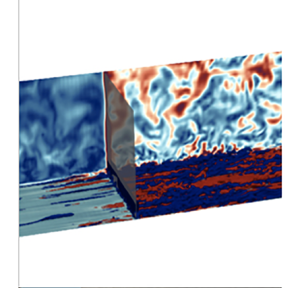
The figure 9 shows iso-contours of streamwise-velocity fluctuations normalised by the local external velocity  $U_e(x,t)$ in a plane parallel to the wall located at
  $y^+_{0} = 5$, in an area close to
  $70\,\%$ chord.

Figure 9. Streamwise fluctuating velocity iso-surfaces normalised by local external velocity  $U_e(x,t)$. Here,
  $x^* = 0$ corresponds to
  $70\,\%$ of the chord and
  $t^*$ is defined as
  $t^* = {t}/({\delta _{(x^*,t)=0}/U_{b,1}})$.
The situation in figure 9 $(a)$ corresponds to the initial flow for which many turbulent structures are visible, showing that the boundary layer is fully turbulent. In figure 9
 $(b)$, the shock is in the analysis region. Immediately behind the shock, the turbulent structures have almost extinguished. Compared with the accelerated velocity of the main flow, the fluctuations are now negligible. Only a few isolated disturbances persist: the flow seems quasi-laminar. After a delay, streamwise elongated streaks appear in figure 9
 $(c)$. Between figure 9
 $(b)$ and figure 9
 $(c)$, pre-existing turbulent structures are modulated to give rise to streaks. The time needed to observe streamwise streaks after the shock propagation can be interpreted as a receptivity process of the boundary layer to pre-existing turbulence. These streaks degenerate to turbulent spots.
The phase between the shock propagation and the first turbulent spots can be named pre-transition in relation with the work of He & Seddighi (Reference He and Seddighi2013) for an incompressible flow. Figure 9(d) reveals the coexistence of turbulent spots with streamwise streaks on the same abscissa: this is the transition stage. Turbulent spots become increasingly prominent during the transition stage, as illustrated on view  $(e)$. This stage ends when the turbulence has totally contaminated the boundary layer: it is then fully turbulent with the properties of the new turbulence, which emerged in figure 9(d). The transition from the old turbulence to the new is therefore not monotonous but follows a temporal transition that has similarities with the spatial bypass boundary layer process. The temporal transition is completed in three stages: pre-transition, transition and fully turbulent boundary layer. These steps exhibit large similarities with the three phases of a bypass spatial process, namely: buffeted laminar boundary layer, transition and fully turbulent boundary layer. Moreover, these steps are very similar to those described by He & Seddighi (Reference He and Seddighi2013) observed in incompressible flow. Compressibility does not seem to significantly affect the turbulence dynamic provoked by an acceleration. The analysis of the mean and fluctuating motion which is now proposed helps to confirm this, as well as to reinforce the similarities with the bypass process.
4.2.2. Mean motion
Figure 10 shows the temporal evolution of the friction coefficient at  $70\,\%$ of the chord (a delay effect due to flow advection is observed when the friction coefficient is extracted at a further abscissa; see, for instance, figure 8(c) to observe this delay). As observed in figure 7, a peak of friction follows the shock, which is here located at
  $(t^*=0^+)$. This peak is provoked by the sudden acceleration of the entire flow, which also generates a thin layer of high strain close to the wall, as we show in the following while analysing the velocity profile. This thin wall shear layer then diffuses into the boundary layer, causing a drop in the friction coefficient. This phase is the pre-transition step
  $(t^*<7.0)$. When the first turbulent spots appear, the friction coefficient begins to increase: this is the beginning of the transition phase
  $(t^*=7.0)$. When the transition ends, the friction is constant at the value corresponding to the
  $Re_{\theta }$ of the final regime
  $(t^*=16.0)$. The temporal evolution of the friction coefficient reveals strong similarities with the spatial development of the friction coefficient of a boundary layer undergoing a bypass transition.

Figure 10. Temporal evolution of the friction coefficient at  $70\,\%$ chord.
To go further in comparison with a spatial case, He & Seddighi (Reference He and Seddighi2013) proposed to investigate the temporal evolution of the boundary layer resulting only from the acceleration (i.e. shock propagation). Consequently, the temporal development of the boundary layer is investigated by examining the differential boundary layer,
 \begin{equation} \bar{u}\hat (
y/\delta, t^*) = \frac{\bar{u}(y/\delta, t^*) -
\bar{u}(y/\delta, 0) }{ U_{b,1} - U_{b,0}},
\end{equation}
\begin{equation} \bar{u}\hat (
y/\delta, t^*) = \frac{\bar{u}(y/\delta, t^*) -
\bar{u}(y/\delta, 0) }{ U_{b,1} - U_{b,0}},
\end{equation}
where  $U_{b,0}$ (
 $U_{b,1}$) represents the external flow velocity for the initial (final) flow.
The graph on the left-hand side of figure 11 represents the differential velocity profile in the boundary layer as a function of  $y/\delta (t)$. Immediately following the wave passage,
  $\bar {u}$ˆ is close to
  $1$ in almost the entire boundary layer except very close to the wall. This means that the acceleration imposed by the shock wave is constant throughout the boundary layer thickness which reacts as a whole, except the very near-wall region. The velocity profile recorded at
  $t^*=0.4$ shows how intense the shear layer is. The diffusion of this layer in the core of the boundary layer is the key phenomenon, initiating many mechanisms during the transient. This diffusion is very clear during the pre-transition phase (between
  $t^*=0.4$ and
  $t^*=7.0$), whereas the differential velocity profile in the outer region of the boundary layer remains essentially unchanged. Then, for
  $t^*>7.0$, the outer regions of the profile are affected, and the wall shear stress starts increasing: the transition phase has begun.

Figure 11. Normalised differential velocity during the transient flow at  $70\,\%$ of chord: blue, pre-transition; red, transition; black, fully turbulent.
The present pre-transition stage looks quite similar to a laminar boundary layer, according to the evolution of the friction coefficient presented previously. This is detailed further and the usual self-similarity of laminar flows are sought, such as that observed for the normalised velocity profile as a function of the normalised wall distance  $\eta = y/\delta (x)$, see Schlichting & Gersten (Reference Schlichting and Gersten2017).
However, the differential velocity profiles ( $\bar {u}\hat {}\,$), plotted against
  $y/\delta (t)$, do not show any self-similarity during this phase. The difficulty comes from the offset introduced by the initial value of the boundary layer thickness. This problem does not exist for conventional spatial analysis of a flat plate boundary layer because the thickness is null at the leading edge. For the present investigation, compensation is required to reveal the self-similarity: subtraction of the initial thickness of the boundary layer is performed so that our fictitious thickness is zero before the shock propagation. The velocity profiles are then displayed as a function of
  $\eta = {y}/({\delta (t) - \delta _0}) = {y}/{\sqrt {\nu t}}$. Figure 11 finally demonstrates that a self-similarity actually exists during the pre-transition stage. The temporal development of the differential boundary layer thus follows a laminar-like growth process during the pre-transition. This is consistent with the instantaneous flow visualisations. Indeed, downstream of the shock wave, despite some pre-existing residual turbulence, no turbulent spots can be observed until the beginning of the transition stage. Only streaks appear during this stage, which is typical of a buffeted laminar boundary layer.
A more direct comparison of the two transitional processes, spatial and temporal, is now proposed in figure 12. It is based on the mean flow features trough the friction coefficient. A reference velocity is required to synchronise those two plots, and have a good correspondence between  $x$ (or here
  $Re_x$) and
  $t^*$. This reference velocity is obtained by minimising the difference between the synchronised temporal friction and the Blasius solution in the quasi-laminar region, which gives a value of
  $0.76U_{b,1}$. The final correspondence between the two mechanisms is striking. The deviation compared with the Blasius laminar prediction is observed at the same location. This suggests that the receptivity of those two boundary layers (stage
  $(0)$ on the figure 12) is quite similar. In the spatial case, it is a receptivity to external disturbances. In the temporal case, a receptivity to the residual old turbulence. The characteristic time of such a receptivity looks comparable in the two cases. Interestingly, the maximum turbulence rate in the initial boundary layer and that of the external flow in the initial spatial case are also comparable. Indeed, the maximum turbulence rate in the initial boundary layer is approximately equal to
  $5\,\%$ (when normalised by the external post-shock velocity) to
  $y^+_0 = 12$, which corresponds to the turbulence rate of the external flow during the initial regime. However, this turbulence is strongly anisotropic in one case, whereas it has isotropic properties in the other. However, the start of the transition phase (stage
  $(2)$ in figure 12) does not happen at the same time (
 $t^*=5.0$ for the spatial case against
  $t^*=7.0$ for the temporal case). This is certainly caused by a change in the mechanism at the origin of turbulent spots. Unlike spatial evolution, when the differential boundary layer becomes fully turbulent, friction becomes constant (stage
  $(3)$ on the figure 12). The transient regime then ends in the near-wall region and the flow there reaches an equilibrium corresponding to the characteristics of the new turbulence.

Figure 12. Temporal evolution of friction coefficient based on differential velocity. Here,  $C_f = {\tau _{w,\hat {u} }}/{1/2\rho U_{b,1}^2}$ with
  $\tau _{w,\hat {u}} = \mu ({\partial [ u(y/\delta,t^*) - u(y/\delta,0) ] }/{\partial y}$.
4.2.3. Fluctuating motion
The response of the fluctuating field, which initiate the different changes in the mean flow, is now detailed. It reinforces the understanding of the different phases of the process which were presented previously.
A representation of Reynolds stresses at  $70\,\%$ of the chord during the establishment transient of the new equilibrium of the boundary layer is given in figure 13. The boundary layer characteristic thicknesses are also reported and the steps of the transitional process recalled. Reynolds stresses are normalised here by the external velocity of the boundary layer and thus reflect the turbulence influence on the mean flow. When the shock crosses the abscissa at
  $t^*=0$, the normalised Reynolds stresses experience a sudden drop and reach a very low level which persists all along the phase
  $(0)$. The turbulence influences on flow dynamics is weak compared with their contribution to the pre-shock flow
  $(t^*<0)$. However, a different normalisation (figure 14) shows that the absolute level of fluctuations is comparable to that of the pre-shock situation. The shock wave accelerates the flow but freezes the intensity of fluctuations at its initial level, all along this first phase (there is actually a very slight amplification of
  $u'_{rms}$ during this phase). This explains why the flow can be considered as quasi-laminar immediately after the wave passage and explains why the differential boundary layer is laminar during this stage. In addition, the receptivity process of the boundary layer to those pre-existing perturbations is underway, and the phase
  $(1)$ begins when the streamwise Reynolds stress
  $(u'_{rms})$ growth is significant.

Figure 13. Reynolds stresses normalised by the external velocity  $(U_e(x,t))$ during the transient flow:
  $(0)$ receptivity process;
  $(1)$ streak growth;
  $(2)$ transition; and
  $(3)$ fully turbulent. Here,
  $(0)$ and
  $(1)$ correspond to the pre-transition stage according to He & Seddighi (Reference He and Seddighi2013).

Figure 14. Production and pressure strain terms for  $u'_{rms}$ integrated over the boundary layer thickness and normalised by
  $\rho u_{\tau,0}^4/(\nu \delta _0)$.
Only the streamwise component takes benefits from a production term (see Cebeci & Cousteix Reference Cebeci and Cousteix2005) which explains why it is the first to respond. However, this response is not instantaneous, despite the very intense shear layer created by the wave near the wall. The production term  $(- \rho \overline {u'v'} ({\partial \bar {U}}/{\partial y}))$ is the product of the normal mean velocity gradient and the turbulent shear stress. The latter is substantially zero near the wall, up to approximately
  $y^+_0=5$. However, pre-existing turbulent structure persists elsewhere in the boundary layer and provides the disturbances on which the new turbulence will emerge. Thus, the delay in the response of
  $u'_{rms}$ is the characteristic time required by the diffusion of the shear layer to reach heights where the turbulent shear stress is no longer negligible. Then the production term is activated and the streamwise elongated streaks form. Stages
  $(0)$ and
  $(1)$, cf. figure 13, correspond to the pre-transition stages according to He & Seddighi (Reference He and Seddighi2013). The increase in the growth rate of the production term as the pre-transition step is shown in figure 15, where the temporal evolution of the production integrated over the boundary layer thickness is given. During pre-transition, the turbulent kinetic energy is therefore essentially concentrated in the streamwise component of the fluctuating motion through streaks. At the end of this step, the turbulence's anisotropy level is, therefore, very high compared with that of an equilibrium turbulent boundary layer.

Figure 15. Reynolds stresses normalised by the post-shock external velocity  $(U_{b,1})$ during the transient flow:
  $(0)$ receptivity process;
  $(1)$ streak growth;
  $(2)$ transition; and
  $(3)$ fully turbulent. Here,
  $(0)$ and
  $(1)$ correspond to the pre-transition stage according to He & Seddighi (Reference He and Seddighi2013).
The pre-transition stage ends as soon as the pressure strain term activates the turbulent kinetic energy redistribution through the responses of  $v'_{rms}$ and
  $w'_{rms}$. These two stresses are thus activated together and indicate the appearance of turbulent spots and the beginning of the transition phase. In the present configuration, the transition starts for
  ${u'_{rms, max}/U_{b,1} \approx 10\,\%}$. This value is in agreement with the critical amplitude predicted by Vaughan & Zaki (Reference Vaughan and Zaki2011) for the streaks, at the beginning of the transition stage for a spatial bypass process. It is also interesting to note that this phase starts exactly at the time predicted by the criterion of He & Seddighi (Reference He and Seddighi2015), so-called
  $t^*_{cr} = 1.34\times 10^3({\nu _1}/{U_{b,1}\delta _0})({u'_{rms,max}}/{U_{b,1}})^{1.71}$. This seems to suggest that, for the study conditions, the temporal Reynolds number of the transition stage beginning is only dependent of initial turbulence intensity and not of the turbulence length scale, in the same way as those described by He & Seddighi (Reference He and Seddighi2015) for the acceleration of an incompressible turbulent boundary layer. This result is not in line with Brandt et al. (Reference Brandt, Schlatter and Henningson2004) findings, which revealed that the transition Reynolds number was dependent on the turbulence length scale for a spatial transition of a boundary layer subject to free-stream turbulence. It should be underlined that the result presented here should be treated with caution as no sensitivity of the results to the turbulence length scale was performed in this study.
In addition, the growth of the maximum of  $u'_{rms}$ is observed inside the transition stage even though the redistribution term is already active. This is another example of similarities with the usual bypass process: it has been observed in figure 6 while analysing the spatial transition of the initial boundary layer. The nature of the structures containing the kinetic energy of the fluctuating motion changes continuously during the transition stage from elongated streaks to small turbulent spots, resulting in changes in the kinetic energy spectrum during this phase.
At stage  $(3)$, the turbulence has contaminated the entire boundary layer thickness. The Reynolds stresses distribution become constant in time: the transition phase is over and a steady equilibrium state is found. The boundary layer is thus fully turbulent. Some boundary layer regions are fully turbulent before others because the response time differs according to the wall distance. This is why the transition appears completed at
  $t^*=16$ according to the friction coefficient, whereas at this stage, the outer region of the boundary layer is still only slightly affected by the new turbulence. In the fully turbulent region, the turbulence in the boundary layer thus recovers typical levels of anisotropy.
Finally, let us closely look at the turbulence dynamic behind the wave, which is also identical to that of a bypass spatial transition of the boundary layer. The temporal evolution of maximum turbulent kinetic energy and Reynolds stresses are presented in figure 16. During a bypass transition, the disturbances amplification is linearly related to the longitudinal distance or  $Re_x$. This linearity is also observed in the temporal domain during the pre-transition stage, which corresponds to the developments of the streaks
  $(t^* \in [2.5, 7.0])$. The different delays in the response of Reynolds stresses are particularly evident.

Figure 16. (a) Disturbances maximum along the plate. (b) Profile of  $u'_{rms}/u'_{rms,max}$ for several
  $Re_x$. Here,
  $U_{b,0}$ corresponds to the boundary layer external velocity of the initial flow.
On the same figure 16, the velocity profiles  $u'_{rms}/u'_{rms,max}$ are also proposed. During a bypass transition, these velocity profiles present a maximum whose distance to the wall is constant throughout the streak amplification phase, see Luchini (Reference Luchini2000). Here, the streak amplification happens when
  $t^* \in [2.5, 7.0]$. In that time interval, the location of this maximum is recorded constant, approximately at
  $y/\delta _u = 0.4$. This is closer to the wall than what is generally observed for a spatial bypass process
  $(y/\delta _u = 1.33)$. This difference probably comes from the location at which the perturbations initiating the streaks are found. For the spatial process, it comes from the free-stream turbulence: the outer part of the boundary layer is thus concerned. For the temporal process, it is the residual old turbulence which triggers the instability. It is thus present at far more important depths inside the boundary layer. However, the fundamental mechanism remains the same.
5. Conclusions and summary
The boundary layer response to a shock wave propagation was examined on the academic case of the flat plate using LES. The temporal development of the whole spatial boundary layer was first described before focusing on the unsteady evolution of the boundary layer in a region where the boundary layer is turbulent during the initial and final steady flow. It has been shown that the shock wave propagation generates a thin wall shear layer whose temporal development is at the origin of the boundary layer changes. The main boundary layer modifications are briefly summarised in chronological order.
Immediately after the shock wave propagation, an intense friction peak is observed, resulting from the interaction between the fluid acceleration in the boundary layer and the no-slip wall boundary condition. The velocity gradient is diffused to the other parts of the boundary layer in the following instants and immediately causes a significant reduction in wall friction. At this stage, the boundary layer appears as quasi-laminar and the differential boundary layer exhibits a laminar behaviour, showing an excellent agreement with Blasius theory. This is confirmed by the freezing of the Reynolds stresses during this phase. The turbulence effect on the flow dynamics becomes negligible. However, the turbulent kinetic energy absolute level remains unchanged from its pre-shock level, so that turbulent structures are still present in the boundary layer. This quasi-relaminarisation phase shows strong similarities with the spatial acceleration of a turbulent boundary layer, see for example Launder (Reference Launder1964) or Sreenivasan (Reference Sreenivasan1982).
The interaction between the velocity gradient and the pre-existing turbulent structures leads to the production of turbulent kinetic energy. Streamwise elongated streaks are then generated and amplified. The previous phase can thus be interpreted as a receptivity process of the boundary layer, toward pre-existing disturbances. This response first occurs close to the wall before diffusing it to the rest of the boundary layer. During this stage, the differential boundary layer begins to deviate from the laminar pattern. The laminar boundary layer is thus buffeted in the same way it does for a bypass spatial transition. This step is characterised by a linear disturbance amplification in the boundary layer. During this step, the  $u'_{rms}$ profile are scaled by the boundary layer displacement thickness and not by the length scale of the inner region, as it is usually the case for a turbulent boundary layer. These behaviours are shared to a bypass process spatial development. However, it was found that the maximum of
  $u'_{rms}$ is located closer to the wall compared with a spatial process. This is most likely because the streaks are located, on average, at lower heights in the boundary layer than during a spatial process. Indeed, unlike a transition process induced by free-stream turbulence, the disturbances at the origin of the temporal transition process do not need to penetrate the boundary layer because they are already there.
The transition stage starts as soon as the first turbulent spots appear. It is found that the onset of the transition step is only dependent of the initial turbulence intensity, according to the same criterion as that developed by He & Seddighi (Reference He and Seddighi2015) for incompressible flows. Spots are generated thanks to the response of the pressure–strain term. This term contributes to taking energy from the streamwise component and redistributing it in the spanwise and normal direction. Streamwise elongated streaks are then destroyed to generate spots. Spots are much more efficient than streaks to promote momentum exchanges between each region of the boundary layer. High velocities are then found close to the wall, which increases the friction coefficient all along the transition. The transition ends when the boundary layer thickness is entirely contaminated by turbulence.
When the boundary layer equilibrium is restored along the plate, the boundary layer transition abscissa is shifted downstream from that of the initial steady flow. The stabilising effect of acceleration on turbulent flow tends to reduce the free-stream turbulence rate, helping to move the transition abscissa away from the leading edge.
It has been demonstrated all along the paper that this temporal transition process is very similar to a bypass process of a spatial transition. The different stages of the process are dictated by the same energy transfer mechanisms from the mean flow to the fluctuating flow, and then toward fluctuating energy redistribution. The trigger of the transition differs, but this does not affect the process drastically.
This boundary layer temporal transition process is essentially the same as that depicted by He & Seddighi (Reference He and Seddighi2013) during the acceleration of an incompressible flow. It means that the compressible effects have a marginal role in the turbulence dynamics inside the boundary layer after the sudden acceleration induced by the shock. A major consequence of the shock intensity increase will be that the spatial boundary layer transition point of the final regime will be moved further downstream, because the final regime turbulence rate will be decreased compared with the simulations performed here.
An interesting perspective would be a generalisation of the investigation regarding sudden accelerations: an expansion wave propagating along negative  $C^-$ characteristic curves would also create an acceleration, but the boundary layer would be expanded instead of being compressed. In addition, the dynamic complexity of turbulence downstream of the wave, due to the time evolution of the anisotropy, is a real challenge for the turbulence models in predicting this kind of flows. The present results constitute an opened database for validation.
Acknowledgements
The authors would like to thank the Direction générale de l'armement (DGA) for their financial support and permitting the research's publication. This work was performed using HPC resources from GENCI-IDRIS and GENCI-CINES on Jean Zay, Occigen (grant A0082A07178) and CALMIP on Olympe (grant 2020-p1425).
Funding
This work was supported by the DGA.
Declaration of interests
The authors report no conflict of interest.


