2.1. Sheet evolution

Unsteady sheet dynamics in the air upon drop impact on a small surface of comparable size to that of the drop was studied in prior works (Rozhkov, Prunet-Foch & Vignes-Adler Reference Rozhkov, Prunet-Foch and Vignes-Adler2002; Villermaux & Bossa Reference Villermaux and Bossa2011; Vernay, Ramos & Ligoure Reference Vernay, Ramos and Ligoure2015; Wang & Bourouiba Reference Wang and Bourouiba2018). Here, we chose the characteristic length scale as impacting drop diameter, $d_0$, and the characteristic time scale as the capillary time, $\tau _{cap} = \sqrt {\rho \varOmega _0/{\rm \pi} \sigma }$, where $\rho$ and $\sigma$ are the fluid density and surface tension, respectively, and $\varOmega _0$ is the impacting drop volume. Thus, the non-dimensional variables are

(2.1a–d)\begin{equation} R = \frac{r}{d_0}, \quad T = \frac{t}{\tau_{cap}}, \quad U = \frac{u}{d_0/\tau_{cap}}, \quad H = \frac{h}{d_0}, \end{equation}

where, $r$ is the radial position in the sheet, $t$ is time, $u$ is the sheet radial velocity and $h$ is the sheet thickness (figure 1). Wang & Bourouiba (Reference Wang and Bourouiba2017) proposed and validated the spatio-temporal thickness $h(r,t)$ and velocity $u(r,t)$ profiles of the thin 2-D sheet, which in non-dimensional form, reads

(2.2a,b)\begin{equation} U(R,T) = \frac{R}{T} \quad \text{and} \quad H(R,T) = \frac{T\sqrt{6We}}{6a_3R^3 +a_2R^2T\sqrt{6We} + a_1RT^2We}, \end{equation}

where $a_1$, $a_2$ and $a_3$ are constant coefficients derived and validated in Wang & Bourouiba (Reference Wang and Bourouiba2017). $We = \rho u_0^2d_0/\sigma$ is the impact Weber number, where $u_0$ is the impacting drop velocity.

Wang & Bourouiba (Reference Wang and Bourouiba2018) showed that the droplets are continuously shed from the thin sheet with most being ejected prior to maximum radial expansion. Wang & Bourouiba (Reference Wang and Bourouiba2020b) showed that the sheet dynamics incorporating unsteadiness and continuous droplet shedding is governed by a non-Galilean Taylor–Culick's law, which, in non-dimensional form, reads

(2.3)\begin{equation} -\!6H(R_s,T)\left(\frac{R_s}{T}-\dot{R_s}\right)^2 + \left(2-\frac{\rm \pi}{7}\right) = 0, \end{equation}

where $H(R_s,T)$ is the sheet thickness at the rim given by (2.2a,b) and $R_s = r_s/d_0$ is the sheet radius. Wang & Bourouiba (Reference Wang and Bourouiba2020b) also derived and validated the approximate analytic solution

(2.4)\begin{equation} \left. \begin{aligned} & \frac{R_s(T)}{\sqrt{We}} =Y(T)= 0.15(T-T_m)^3-0.4(T-T_m)^2 + \mathcal{R}_m,\\ & \text{with} \ T_m = 0.43 \quad \text{and} \quad \mathcal{R}_m = R_m/\sqrt{We} = 0.12, \end{aligned} \right\} \end{equation}

where $R_m$ is the maximum radius of the sheet in the air and $T_m$ is the time when this maximum radius is reached.

2.2. Rim destabilization and fluid volume shed

The critical first link between the sheet evolution and the ligaments that shed secondary droplets via end-pinching is the rim destabilization into corrugations. Due to mathematical complexity, traditional theoretical studies of rim destabilization conducted linear instability analysis, examining whether the Rayleigh–Plateau instability (Rayleigh Reference Rayleigh1878; Deegan, Brunet & Eggers Reference Deegan, Brunet and Eggers2008; Roisman Reference Roisman2010; Zhang et al. Reference Zhang, Brunet, Eggers and Deegan2010; Agbaglah, Josserand & Zaleski Reference Agbaglah, Josserand and Zaleski2013; Agbaglah & Deegan Reference Agbaglah and Deegan2014) or the Rayleigh–Taylor instability (Taylor Reference Taylor1950; Villermaux & Bossa Reference Villermaux and Bossa2011; Peters, Meer & Gordillo Reference Peters, van der Meer and Gordillo2013) dominates the rim destabilization. Recent studies via numerical simulation (Roisman Reference Roisman2010; Agbaglah et al. Reference Agbaglah, Josserand and Zaleski2013) showed that the nonlinearity plays a key role in the rim destabilization. To elucidate and quantify the linear and nonlinear effects at first order, we (Wang & Bourouiba Reference Wang and Bourouiba2018) showed that the rim initially destabilizes into small corrugations due to the interplay of a coupled instability where both acceleration and interfacial constraints on the rim play key roles. However, when the corrugations grow to a certain size, nonlinear effects dominate, associated with an instantaneous self-adjustment of the rim thickness, $b$, for it to remain equal to the local capillary length, $\ell _c$, defined based on the instantaneous rim deceleration, $\ddot {r_s}$, by $\ell _c = \sqrt {\sigma /(\rho (-\ddot {r_s}))}$, where $\rho$ and $\sigma$ are the density and surface tension of the fluid, respectively. Namely, the rim thickness is selected to maintain a local and instantaneous Bond number $Bo = \rho b^2 (-\ddot {r_s})/\sigma = 1$. Such a $Bo = 1$ constraint on the rim thickness is robust and independent of the impact Weber number. Using the $Bo = 1$ criterion, Wang & Bourouiba (Reference Wang and Bourouiba2020a) showed and validated that the rim thickness $b$ scales as $We^{-1/4}$ with the approximate analytic expression, in non-dimensional form,

(2.5)\begin{equation} B(T) = \frac{b}{d_0} = We^{-1/4}\varPsi(T) \quad \text{with} \ \varPsi(T) = -0.68T^2 + 0.94T + 0.18. \end{equation}

Note that the coefficients of (2.5) are theoretically derived, not fitted. The universal $Bo = 1$ criterion governing the rim links the unsteady non-Galilean sheet evolution (2.3) with the fluid shedding in the form of ligaments and droplets. Wang & Bourouiba (Reference Wang and Bourouiba2020a,Reference Wang and Bourouibab) showed and validated that the volume shed from the rim per unit of time, and radian, $q_{out}$, is determined by the mass balance between the fluid entering the rim per unit of time, and radian, $q_{in}$, and continuous self-adjustment of the rim thickness to balance inertial and capillary forces via the unsteady local $Bo = 1$ criterion (Wang et al. Reference Wang, Dandekar, Bustos, Poulain and Bourouiba2018c), such that

(2.6)\begin{equation} \left. \begin{aligned} q_{out}(t) & = q_{in}(t) - \frac{d}{dt}\left(\frac{\rm \pi}{4}b^2 r_s \right) \quad \text{with}\\ q_{in}(t) & = \rho h(r_s,t)[u(r_s,t)-\dot{r_s}]r_s(t) \quad \text{and} \quad b = \frac{\sigma}{\rho(-\ddot{r_s})}, \end{aligned} \right\} \end{equation}

where $r_s(t)$ is given by (2.4), and $h(r_s,t)$ and $u(r_s,t)$ are the sheet thickness and velocity profiles evaluated at the rim, i.e. at $r = r_s$ (Wang & Bourouiba Reference Wang and Bourouiba2020b). It was shown (Wang & Bourouiba Reference Wang and Bourouiba2020a) that $q_{out}$ is in fact independent of $We$ over the capillary time scale $\tau _{cap}$, with the approximate analytic expression, in non-dimensional form,

(2.7)\begin{equation} Q_{out}(T) = \frac{q_{out}}{d_0^3/\tau_{cap}} = 0.15T + 0.03. \end{equation}

Note here too that the coefficients were theoretically derived, not fitted. We show later (§ 6) that such volume shed by the rim per unit of time, $q_{out}$, is in fact the key determinant in the selection of corrugations that can eventually grow into ligaments and shed droplets.

2.3. Droplet ejection

Riboux & Gordillo (Reference Riboux and Gordillo2014) stated that both the size and speed of the droplets shed from expanding sheets are equivalent to the size and speed of the expanding rim, respectively. Wang et al. (Reference Wang, Dandekar, Bustos, Poulain and Bourouiba2018c) showed that the properties of secondary droplets are, in fact, governed by the end-pinching of ligaments, shedding one drop at a time, with population average diameter and speed set by the ligaments, rather than the rim. Two universal relations between the ligaments and droplets were established (Wang et al. Reference Wang, Dandekar, Bustos, Poulain and Bourouiba2018c). First, the ratio of the diameter, $d$, of each secondary droplet with the width of its ligament of origin, $w$, is $d/w \approx 1.5$, which remains constant throughout the sheet fragmentation, and is independent of $We$. Second, the ejection speed of each secondary droplet, $u_d$, is equal to the tip speed of its ligament of origin, $u_{\ell }$, one necking time, $t_{neck}$, prior to end-pinching, namely

(2.8)\begin{equation} u_d(t) = u_{\ell}(t-t_{neck}) \quad \text{with} \ t_{neck} = 3.2\sqrt{\frac{\rho w^3}{8\sigma}}. \end{equation}

2.4. Inviscid regime

Here, we note that the unsteady sheet fragmentation theory including that of the dynamics of the sheet (§ 2.1) (Wang & Bourouiba Reference Wang and Bourouiba2020b), the rim (§ 2.2) (Wang et al. Reference Wang, Dandekar, Bustos, Poulain and Bourouiba2018c) and the ligaments (this paper), is developed for the inviscid regime governed by the balance between fluid inertia and surface tension. Wang et al. (Reference Wang, Dandekar, Bustos, Poulain and Bourouiba2018c) showed that when the Reynolds number of the rim $Re_b = v_b b/\nu < 6\sqrt {2}$, viscous effects mitigate rim destabilization, as well as ligament growth and breakup. Here, $b$ is the rim thickness, $\nu$ is the fluid kinematic viscosity and $v_b = \sqrt {\sigma /\rho b}$ is the characteristic speed of corrugation growth. For $Re_b = v_b b/\nu < 6\sqrt {2}$, the $Bo = 1$ criterion of the rim no longer holds. Thus, the boundary conditions at the rim that determine the ligament dynamics, such as the total volume rate shed by the rim $q_{out}$, would differ from (2.7). An extension of the theory combining inertia, viscosity and surface tension beyond what is discussed in this paper, would be required in this regime for capturing and predicting the ligament evolution.

3.1. Experimental conditions

For each experiment, an impacting drop of diameter, $d_0$, is released by a needle from different heights to set different impacting speeds, $u_0$. Two high speed cameras are used to record the experiments from side and top views. The diameter and impacting speed of the drop are directly measured from the side view. The frame rate of the top-view and side-view cameras are 20 000 and 8000 frames per second (f.p.s.), respectively. The pixel resolution of videos recorded from top and side views are ${\simeq} 50\ \mathrm {\mu }\textrm {m}\,\textrm {pixel}^{-1}$ and ${\simeq } 30\ \mathrm {\mu }\textrm {m}\,\textrm {pixel}^{-1}$, respectively. Drops are made of de-ionized water and Nigrosine dye of concentration of $1.2\ \textrm {g}\,\textrm {l}^{-1}$, with density $\rho = 1.0 \times 10^3\ \textrm {kg}\,\textrm {m}^{-3}$, surface tension $\sigma = 72 \times 10^{-3}\ \textrm {N}\,\textrm {m}^{-1}$ and kinematic viscosity $\nu = 1.0 \times 10^{-6}\ \textrm {m}^2\,\textrm {s}^{-1}$. The surface of the rod is made of stainless steel with contact angle range between $52^{\circ}\text{ and } 81^{\circ}$ (McMaster 304 Stainless steel with 000-Grit sand-paper polishing). The diameter of the rod is selected to ensure a rod-to-drop size ratio, $1.4<\eta = d_r/d_0<1.9$, within the range ensuring a horizontal sheet and negligible effect of surface stresses (Wang & Bourouiba Reference Wang and Bourouiba2017). To confirm the robustness of experimental results, as well as to obtain standard deviations, 28 videos are taken for each group of centred impact experiment. Two dimensionless groups relevant to our impact conditions are the Weber number, $We=\rho u_0^2d_0/\sigma$, and the Reynolds number $Re = u_0d_0/\nu$, respectively. Detailed experimental conditions are summarized in table 1.

Table 1. Summary of the experimental conditions used for water drop impacts on a rod, including the impact drop diameter, $d_0$, impacting speed, $u_0$, and associated $We = \rho u_0^2 d_0/\sigma$ and $Re= u_0d_0/\nu$, where $\rho = 1.0\times 10^3\ \textrm {kg}\,\textrm {m}^{-3}$, $\nu = 1.0\times 10^{-6}\ \textrm {m}^{2}\,\textrm {s}^{-1}$ and $\sigma = 72\ \textrm {mN}\,\textrm {m}^{-1}$, are the density, kinematic viscosity, and surface tension of the water drop, respectively. $N_{exp}$ is the number of experiments carried out for each group. $d_r$ is the diameter of the impact rod. $\eta$ is the ratio of the diameter of the surface, $d_r$, with that of the impact drop, $d_0$.

3.2. Advanced image processing algorithms

Due to the rich complexity of the corrugation and ligament dynamics (figure 1), we used especially developed advanced image processing (AIP) algorithms (Wang & Bourouiba Reference Wang and Bourouiba2020b) to measure a range of key quantities. The work flow and validation of our AIP algorithms start with a first step of detection of the inner and outer contours of the rim–ligament system (figure 2$a$). The second step is the separation of the ligaments from the rim based on local morphological analysis (figure 2$b$). With the accurate rim–ligament separation, the AIP algorithms can capture the global (population) information of ligaments along the rim directly and automatically, including their number and population average size evolution over time. Finally, each ligament on the rim is tracked over time, linking its size and position at different times throughout the entire sheet evolution (figure 2$c$). The detailed measurements of key ligament dynamics quantities are described in subsequent sections.

Figure 2. Key steps of our AIP algorithms: ($a$) detection of inner and outer contours of the rim–ligament system; ($b$) morphological analysis of the rim–ligament system and the separation of the ligaments from the rim. The inset illustrates the high accuracy of the automatic separation between the rim and the ligaments conducted; ($c$) the ligament-tracking algorithm links the ligaments detected at different frames to form their trajectories.

4.1. Corrugations and rim destabilization

As discussed in § 2, initial corrugations are formed by rim destabilization, the onset of which is governed by a coupled Rayleigh–Plateau (RP) and Rayleigh–Taylor (RT) instability. When the corrugations grow to a certain size, nonlinear effects dominate, associated with a self-adjustment of the rim thickness to maintain a local and instantaneous Bond number $Bo = 1$ (§ 2.2). However, during the entire sheet fragmentation, new corrugations continuously form on the rim. Even though the rim is governed by the $Bo = 1$ criterion, a nonlinear dynamics, the formation of new corrugations on the rim at each time is well captured by a coupled Rayleigh–Plateau and Rayleigh–Taylor instability, the dispersion relation of which, for $Bo = 1$, approaches that of the Rayleigh–Plateau instability. This is consistent with the results in the literature (Deegan et al. Reference Deegan, Brunet and Eggers2008; Roisman Reference Roisman2010; Zhang et al. Reference Zhang, Brunet, Eggers and Deegan2010; Agbaglah et al. Reference Agbaglah, Josserand and Zaleski2013).

Prior studies reported factors that can influence the dispersion relation of the instability of the rim, including the attachment of the expanding sheet to the rim (Roisman et al. Reference Roisman, Gambaryan-Roisman, Kyriopoulos, Stephan and Tropea2007; Agbaglah et al. Reference Agbaglah, Josserand and Zaleski2013), and the rim thickening during the sheet evolution (Zhang et al. Reference Zhang, Brunet, Eggers and Deegan2010). Here, the rim thickness is measured by contour detection (figure 3$b$). The sheet thickness $h(r,t)$ is measured using light absorption, with the intensity response of Nigrosine-dyed liquid to the liquid thickness quantified (Wang & Bourouiba Reference Wang and Bourouiba2017) and shown to follow Beer–Lambert's law of absorption $h = \epsilon \log (I_0/I)$, where $I_0$ is the background light intensity, $I$ is the intensity of light after passing through the dyed liquid film, $\epsilon$ is the fluid absorptivity based on dye property and concentration, which we calibrated.

Figure 4($a$) shows that the ratio of the sheet thickness at the rim, $h(r_s,t)$, with the rim thickness, $b(t)$, remains much smaller than 1 during the entire sheet evolution. In this regime, prior numerical work (Agbaglah et al. Reference Agbaglah, Josserand and Zaleski2013) showed that the sheet attachment to the rim has a negligible effect on destabilization. Namely, the rim can be considered as a standalone cylindrical liquid column. Figure 4($b$) shows the time evolution of the measured rim thickening time scale $\tau _h = b/\dot {b}$, the ratio of the rim thickness over its rate of change, compared with the time scale of the fastest-growing mode of the Rayleigh–Plateau instability, $\tau _{is} = 0.343\sqrt {\rho b^3/(8\sigma )}$ based on the instantaneous measured rim thickness. Figure 4($b$) shows that, during the entire sheet evolution, $\tau _{h} \gg \tau _{is}$. Even at early time, the rim thickening time scale is still twice as large as the instability time scale. Thus, the rim can be considered as quasi-static for the purpose of analysing the local dynamics of onset of rim instability over a given time snapshot.

Figure 4. ($a$) Time evolution of the ratio, $\kappa (t)$, of the sheet thickness at the rim, $h(r_s,t)$, with the rim thickness $b(t)$ for impact $We = 679$ and rod-to-drop size ratio $\eta = 1.45$, showing that $\kappa (t) \ll 1$ during the entire sheet evolution. ($b$) Time evolution of the instability time scale, $\tau _{is}$, of the fastest-growing mode of the coupled RP–RT instability of the rim, compared with the rim thickening time scale, $\tau _h$, based on both the volume influx entering the rim and the stretching of the rim length (sheet perimeter) for the same experimental condition as ($a$). It shows that the instability time scale is much slower than the actual thickening.

Based on figure 4, the average distance between the corrugations on the rim should be equal to the wavelength of the fastest-growing mode of the coupled RP–RT instability, which for $Bo = 1$, is close to that of the Rayleigh–Plateau instability (Wang et al. Reference Wang, Dandekar, Bustos, Poulain and Bourouiba2018c): $\lambda _{RP} = 9(b/2) = 4.5b$ (Rayleigh Reference Rayleigh1878). Thus, the total number of corrugations on the rim would be

(4.1)\begin{equation} N_c(T) = \frac{2{\rm \pi} r_s}{\lambda_{RP}} = \frac{4{\rm \pi} R_s(T)}{9B(T)}, \end{equation}

where $R_s = r_s/d_0$ and $B = b/d_0$ are the dimensionless sheet radius and rim thickness, respectively, non-dimensionalized by the impacting drop diameter $d_0$. The evolution of $R_s(T)$ and $B(T)$ were derived in Wang & Bourouiba (Reference Wang and Bourouiba2020a,Reference Wang and Bourouibab) and recalled in § 2.1.

The experimental measurement of the number of corrugations was conducted by detecting and enumerating the number of protrusions, namely, the local maxima of distance between inner and outer contours (figure 3$a$) obtained for each azimuthal angle, $\theta$, along the contour, from $-{\rm \pi}$ to ${\rm \pi}$. However, we note that the pixelization of the image, as well as errors in local contour detection can generate artificial local maxima. To guarantee accurate detection of local maxima free of spurious measurements, we consider a local maximum to be a true protrusion if the local rim thickness of the local maximum is larger than the averaged rim thickness along the entire rim plus the standard deviation of the rim thickness. In addition, we also track each local maximum and capture its evolution over time at a frame rate (20 000 f.p.s.) that is larger than the corrugation growth or decay rate. Thus, if the trajectory of a local maximum only persists for one frame, such a maximum is also discarded from the corrugation count, as it is considered spurious.

A precise measurement for the number of ligaments on the rim is also required. A manifest feature of a ligament distinct from a corrugation is that it eventually sheds droplets. However, this cannot be used as a criterion to count the number of ligaments. Indeed, the shedding of a droplet from a ligament occurs only in one instant, without information about its history and persistence prior and post shedding. Instead what clearly distinguishes a ligament from a corrugation is that a ligament is a growing protrusion with increasing volume over time. Note that with a volume increase, given the fictitious inertial force, ligaments are also characterized by an increasing length (between droplet shedding events). A corrugation can also be measured to occasionally deform and increase in length, but not increase in volume. We can summarize the fate of corrugations in three scenarios:

1. (i) A corrugation can transition immediately into a ligament upon formation, by increasing in volume.

2. (ii) A corrugation can maintain a constant volume, remaining a corrugation throughout its lifetime, before either disappearing, or being absorbed by neighbouring drifting ligaments.

3. (iii) A corrugation can remain a corrugation of constant volume for an extended period of time, and then suddenly transition into a ligament, i.e. increase in volume.

Given the above definitions, a precise measurement of the number of ligaments over time consists in measuring the number of protrusions on the rim that are increasing in volume at that time. Our AIP algorithms track all protrusions on the rim and examine the time evolution of their volume and length. At each time, based on the tracking results, a protrusion with increasing volume is classified as a ligament at that time. Those without change in volume are classified as non-growing, i.e. corrugations.

Figure 5($a$) shows the time evolution of the measured number of corrugations (including ligaments), compared to the prediction (4.1), which captures the data very well. However, as discussed earlier, not all corrugations can evolve into ligaments (figure 5$b$). By observation, the physical picture that emerges is that the number and size of ligaments on the rim are constrained by the available fluid volume shed by the rim per unit of time. Indeed, figure 5($b$) shows the measured time evolution of the number of ligaments, $N_{\ell }$, growing on the rim, compared with the measured number of corrugations, $N_c$, for $We = 679$. The number of ligaments is systematically smaller than the number of corrugations, consistent with a restriction on corrugation growth into ligament. Thus, the number of ligament, as well as other properties of ligaments, cannot be captured by linear stability analysis as we discuss next.

Figure 5. ($a$) Time evolution of the number of corrugations, including ligaments, on the rim, compared with the prediction (4.1) from the wavelength of the fastest-growing mode of the Rayleigh–Plateau instability for different Weber numbers. ($b$) Time evolution of the measured number of ligaments, compared with the measured number of corrugations as shown in ($a$) for $We = 679$. The number of ligament is systematically smaller than that of the corrugation, indicating, at each time, that not all corrugations can grow into ligaments. Error bars indicate the standard deviation from 28 experiments for each condition (table 1).

4.2. Linear stability analysis does not govern ligament growth

Figure 6($a$) shows a schematic diagram of the growth of a perturbation on the rim based on linear stability analysis. The evolution of the perturbation could be governed by the fastest-growing mode growth rate of the instability. As discussed in § 2.2, when the rim thickness is governed by the $Bo = 1$ criterion, the initial growth of a corrugation is governed by

(4.2a,b)\begin{equation} \lambda_{RP} = \frac{2{\rm \pi}}{0.7}\ \frac{b}{2} \approx 4.5b \quad \text{and} \quad \omega_{RP} = 0.343\sqrt{\frac{8\sigma}{\rho b^3}} \approx \sqrt{\frac{\sigma}{\rho b^3}}, \end{equation}

where $b$ is the rim thickness, in which case, the width of the corrugation is $\lambda _{RP}/2$ and its length (figure 6) reads as

(4.3a,b)\begin{equation} w = \frac{\lambda_{RP}}{2} = 2.3b \quad \text{and} \quad \ell = \ell_0 \exp\left(\omega_{RP} t\right), \end{equation}

where $\ell _0$ is the initial perturbation amplitude (figure 6$a$). Figures 6($b$) and 6($c$) show that the predictions from linear instability theory (4.3a,b) systematically overestimate the ligament width and length. Such disagreements between predictions and experiments confirm the invalidity of linear stability analysis for the prediction of the ligament growth, the result of a nonlinear process. Indeed, when a corrugation grows into a finite size, detailed analysis of the forces acting on the ligament attached to the rim becomes required.

Figure 6. ($a$) Schematic diagram of corrugation growth based on linear stability analysis. The corrugation width is half of the wavelength of the fastest-growing mode of the linear instability, and the length is the amplitude of the perturbation, following an exponential growth. ($b$) Time evolution of the measured population mean width of a single ligament for impact $We = 693$, compared with the prediction (4.3a,b). ($c$) Time evolution of the measured population average length of ligaments for $We = 693$, compared with prediction (4.3a,b). The ligament length is normalized by the initial measured length of the ligament $\ell _0$, which can be considered as the initial amplitude of the rim's perturbation. Time is non-dimensionalized by the local capillary time, $\tau _b = \sqrt {\rho b^3/8\sigma }$, based on the local rim thickness around the ligament.

5.1. Literature review of single jet dynamics

Prior jet studies focused on jets emitted from a solid orifice or nozzle with fixed flow rate. Figure 7($a$) shows a schematic diagram of a jet emanating from a fixed orifice of inner diameter, $w$, with flow rate, $q_{\ell }$. Due to its cylindrical shape, the ligament would be subject to the Rayleigh–Plateau instability. Taking an initial perturbation of amplitude $\delta _0$ and the fastest-growing mode of the Rayleigh–Plateau instability $\omega _{RP} = 0.343\sqrt {8\sigma /(\rho w^3)}$, the time evolution of the perturbation amplitude would read

(5.1)\begin{equation} \delta(t) = \delta_0 \exp{(\omega_{RP} t)}. \end{equation}

Assuming the ligament breaks up at the time when the perturbation amplitude reaches the radius of the ligament, the time of instability growth is

(5.2)\begin{equation} t_{break} = \frac{1}{\omega_{RP}}\ln{\frac{w}{2\delta_0}} = 2.91\sqrt{\frac{\rho w^3}{8\sigma}}\ln{\frac{w}{2\delta_0}}. \end{equation}

Assuming that the fluid entering the jet has a constant speed, $v_{\ell }$, the breakup length of the ligament is

(5.3)\begin{equation} \ell_b = v_{\ell} \ t_{break} = 1.03w \sqrt{\frac{\rho v_{\ell}^2 w}{\sigma}}\ln{\frac{w}{2\delta_0}}. \end{equation}

However, the above derivation neglects the retraction of the tip of the ligament due to surface tension and the body forces exerted on the ligament, such as gravity or a fictitious force when the ligament is in a non-Galilean frame of reference.

Figure 7. ($a$) Schematic diagram of a jet emanating from an orifice. ($b$) Schematic diagram for a classic ligament analysis, selecting a control volume at the tip of the ligament (§ 5.1).

A more physically sound model for the jet ejection from a solid orifice can be derived by choosing the control volume as the jet's tip on which mass conservation and momentum balance are applied. Remaining in the reference frame of the orifice, and taking the fluid speed, $v_{\ell }$, entering the jet to be constant and taking a constant average jet width away from the tip, mass conservation at the tip reads

(5.4)\begin{equation} \frac{\textrm{d}m}{\textrm{d}t} = \rho A \left(v_{\ell}-\frac{\textrm{d}z}{\textrm{d}t}\right), \end{equation}

where $A = ({{\rm \pi} }/{4})w^2$ is the jet's cross-sectional area, $z$ is the position of the tip and $\textrm {d}z/\textrm {d}t$ is the tip velocity. The momentum balance at the tip reads

(5.5)\begin{equation} \frac{\textrm{d}}{\textrm{d}t}\left(m\frac{\textrm{d}z}{\textrm{d}t}\right) = mg - {\rm \pi}w\sigma + pA + \rho A v_{\ell}\left(v_{\ell} - \frac{\textrm{d}z}{\textrm{d}t}\right), \end{equation}

where $g$ is the body force exerted on the ligament and $p$ is the curvature pressure in the jet. Assuming a cylindrical shape, $p = 2\sigma /w$. By substituting (5.4) into (5.5) and rearranging gives

(5.6)\begin{equation} m\frac{\textrm{d}^2 z}{\textrm{d}t^2} - \rho A\left(v_{\ell} - \frac{\textrm{d}z}{\textrm{d}t}\right)^2 + \frac{1}{2}{\rm \pi} w \sigma - mg = 0. \end{equation}

With the physical restriction of the solid wall, the width of the jet emanating from the orifice is equal to the diameter of the orifice, which is known. Thus, with the initial position and volume of the tip, we can directly derive the evolution of the growth of the jet. However, the base of the ligaments growing on the rim does not have a fixed width. The ligament width remains unknown. Namely, during its deformation, both the length, $\ell$, and width, $w$, change over time. Thus, the prediction of ligament dynamics requires elucidating the local rim–ligament dynamics discussed next.

5.2. Modified theory of ligament growth on a rim

5.2.1. Physical picture

What is the criterion by which an initial perturbation/corrugation can grow into a ligament? Figure 8 shows the typical steps of growth of a corrugation into a ligament. We can see that at first, due to rim destabilization governed by the coupled Rayleigh–Plateau Rayleigh–Taylor instability (§ 4.1), an initial perturbation (figure 8a i) gradually grows thicker to become a corrugation (figure 8a ii) of which the protruded height, $h_c$, is on the same order of magnitude as that of the rim thickness.

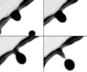
Figure 8. ($a$) Sequence illustrating the growth of a ligament from initial perturbation to a corrugation that is finally pulled away from the rim to form a long ligament in the reference frame of the rim. Time increment between images is 0.5 ms. Scale bar is 0.5 mm. ($b$) Schematic diagram of the model of ligament growth from corrugation without solid-boundary constraints at its root (§ 5.2.2). ($c$) Schematic diagram of the reduced model of ligament dynamics (§ 5.2.3).

We analyse the ligament dynamics in the reference frame of the rim. Recall that, during the entire unsteady sheet fragmentation, the rim is continuously decelerating due to the pull of surface tension acting on the rim at the rim–sheet junction, with the rim acceleration, $\ddot {r_s}$, following the $Bo = \rho b^2 (-\ddot {r_s})/\sigma = 1$ criterion (§ 2.2) (Wang et al. Reference Wang, Dandekar, Bustos, Poulain and Bourouiba2018c). Thus, the reference frame of the rim is a non-Galilean frame, where the rim acceleration, $\ddot {r_s}$, is a fictitious body force, $f_c$, acting on the rim in the direction opposite to that of the rim's acceleration. The rim continuously decelerates, with an acceleration vector pointing radially inward toward the centre of the sheet. Thus, the fictitious force points radially outward: $f_c = -\ddot {r_s}$, which pushes the fluid outward, away from the rim.

When the mass of the corrugation $m_g$ grows further, such a fictitious outward force, $m_g f_c = m_g(-\ddot {r_s})$, becomes eventually larger than surface tension, the fluid in the corrugation is pulled away from the rim (figure 8a iv) and becomes an obtuse protrusion. After that, under the effect of both surface tension and the acceleration force, the protrusion deforms further into an elongated ligament (figure 8a v). When the ligament is formed, its tip grows into a bulged shape due to surface tension (figure 8a vi). Finally, after the bulge forms, the neck between the bulged tip and the root of the ligament appears, and exacerbate until the tip breaks away into a secondary droplet.

5.2.2. Full model of ligament growth

The difficulty of the analysis of ligament dynamics lies in the complex deformation of its shape due to capillary forces. Figure 8($b$) shows a schematic diagram of ligament growth on a rim. For simplicity, we assume that during its growth, the ligament remains axisymmetric and cylindrical. We define $r$ as the radial direction along the width of the ligament, and $z$ as the direction of the ligament length which is perpendicular to the rim. We define $v_{\ell }$ as the speed of fluid emanating from the rim into the ligament during its growth. By choosing a control volume around the entire ligament, mass conservation reads

(5.7)\begin{align} \frac{\textrm{d}m(t)}{\textrm{d}t} = \frac{\textrm{d}}{\textrm{d}t}\int_0^{\ell(t)} \rho A(z,t)\,\textrm{d}z = \rho q_{\ell}(t) = \rho A(0,t)v_{\ell}(t) \quad \text{with}\ A(z,t) = \frac{\rm \pi}{4}w^2(z,t), \end{align}

where $w(z,t)$ and $A(z,t)$ are the local instantaneous width (diameter) and cross-sectional area of the ligament at height $z$ and time $t$, respectively. $\ell (t)$ is the instantaneous total length of the ligament at time $t$. $q_{\ell }(t)$ is the instantaneous rate of fluid volume entering the ligament, expressed by the product of the cross-sectional area of the ligament, $A(0,t)$, and the fluid influx speed, $v_{\ell }(t)$. In addition, momentum balance at the ligament gives

(5.8)\begin{equation} \underbrace{\frac{\textrm{d}}{\textrm{d}t}\int_0^{\ell(t)} \rho A(z,t)u(z,t)\,\textrm{d}z}_{\text{inertia}} = \underbrace{\rho q_{\ell}v_{\ell}}_{\text{momentum influx}} -\underbrace{{\rm \pi} w(0,t) \sigma + p A(0,t)}_{\text{surface tension}} + \underbrace{m(-\ddot{r_s})}_{\text{fictitious force}}, \end{equation}

where $u(z,t)$ is the fluid velocity profile in the ligament along the $z$-direction; $\rho q_{\ell } v_{\ell }$ is the momentum influx entering the ligament; ${\rm \pi} w(0,t) \sigma$ is the surface tension force acting on the root of the ligament pulling it toward the rim; $p A(0,t)$ is the pressure force acting on the root cross-section, $A(0,t)$, of the ligament, induced by the local curvature there. Such a term was initially neglected by prior studies aiming to predict the retraction speed of ligament tips (Keller Reference Keller1983; Clanet & Lasheras Reference Clanet and Lasheras1999), but was subsequently shown experimentally to be important in the dynamics of a cylindrical liquid column (Hoepffner & Paré Reference Hoepffner and Paré2013). Here, $m(-\ddot {r_s})$ is the fictitious body force introduced by the non-Galilean frame of the rim (Wang & Bourouiba Reference Wang and Bourouiba2020b).

The mass and momentum balance equations (5.7) and (5.8) are still not closed. First, the speed $v_{\ell }$ of fluid entering the ligament remains unknown. Second, with no physical constraint, the width of the ligament, $w(z,t)$, on the rim remains unknown. It is non-uniform along the ligament height, $z$, and also changes with time $t$. Third, the fluid velocity profile, $u(z,t)$, in the ligament remains unknown as well.

Assuming $v_{\ell }$ to be known, which we will discuss in § 5.4, the fluid velocity profile $u(z,t)$ in the ligament can be determined by continuity

(5.9)\begin{equation} \frac{\partial}{\partial t}A(z,t) + \frac{\partial}{\partial z}[A(z,t)u(z,t)] = 0. \end{equation}

The kinematic boundary condition at the free surface of the ligament gives

(5.10)\begin{equation} \frac{\textrm{D}}{\textrm{D}t}[r-w(z,t)/2] = 0, \end{equation}

where $\textrm {D}/\textrm {D}t$ is the material derivative in cylindrical coordinates. To determine the full geometric evolution of the ligament, the full system (5.7)–(5.10) would have to be solved numerically. However, to gain physical insights and tractable predictions, we next reduce further the model to capture the leading-order geometric evolution of the ligament analytically.

5.2.3. Reduced analytical model of ligament growth

The core insight is that the variation of thickness along the ligament is actually small (figure 8$a$). Here, we thus neglect the variation of the ligament width $w(z,t)$ along its length (figure 8$c$). The ligament, thus, becomes approximately a cylinder of uniform width $\bar {w}$ at each time. Physically, the uniform width can be considered to be the width of the original ligament averaged along its central axis (figure 8$c$)

(5.11)\begin{equation} \bar{w}(t) = \sqrt{\frac{4}{\rm \pi}\bar{A}(t)} \quad \text{with} \ \bar{A}(t) = \frac{1}{\ell(t)}\int_0^{\ell(t)}A(z,t)\,\textrm{d}z, \end{equation}

where $\bar {A}(t)$ is the average cross-sectional area of the ligament along its central axis. For reduced cumbersomeness, we drop the symbol ‘$\ \bar{}\ $’ from $\bar {w}$ and $\bar {A}$ hereafter; $w(t)$ now represents the average width along the ligament, which depends only on time. The mass of the ligament is thus

(5.12)\begin{equation} m_{\ell}(t) = \int_0^{\ell(t)} \rho {A}(t)\,\textrm{d}z = \rho \frac{\rm \pi}{4} {w}^2(t)\ell(t), \end{equation}

which reduces the mass conservation equation (5.7) to

(5.13)\begin{equation} \frac{\textrm{d}}{\textrm{d}t}\left(\frac{\rm \pi}{4}w^2 \ell\right) =q_{\ell} = \frac{\rm \pi}{4}w^2v_{\ell} \quad \Longrightarrow \quad \frac{\textrm{d}\ell}{\textrm{d}t} + \frac{2\ell}{w}\frac{\textrm{d}w}{\textrm{d}t} = v_{\ell}. \end{equation}

The continuity equation can then be simplified to

(5.14)\begin{equation} \frac{\textrm{d}}{\textrm{d}t}A(t) + A(t)\frac{\partial}{\partial z}u(z,t) = 0 \quad \Longrightarrow \quad \frac{\textrm{d}w}{\textrm{d}t}+ \frac{w}{2}\frac{\partial u}{\partial z} = 0. \end{equation}

Using (5.13) and (5.14),

(5.15)\begin{equation} \frac{\partial u}{\partial z} = -\frac{2}{w}\frac{\textrm{d}w}{\textrm{d}t} = \frac{1}{\ell}\left(\frac{\textrm{d}\ell}{\textrm{d}t} - v_{\ell}\right). \end{equation}

Since both $\ell$ and $v_{\ell }$ are independent of $z$, we take the integral over $z$ on both sides of (5.15), which gives

(5.16)\begin{equation} u(z,t) = \frac{z}{\ell}\left(\frac{\textrm{d}\ell}{\textrm{d}t} - v_{\ell}\right) + u(0,t), \end{equation}

where $u(0,t)$ is the fluid velocity at the root of the ligament, equal to the speed of fluid entering the ligament, namely, $u(0,t) = v_{\ell }(t)$.

Under the uniform-width approximation we made, the variation of the ligament width along its length is neglected. Thus, the kinematic boundary condition (5.10) that governs the free surface become trivial. Finally, the momentum balance (5.8), based on uniform-width approximation, simplifies to

(5.17)\begin{equation} \frac{\textrm{d}}{\textrm{d}t}\int_0^{\ell(t)} \rho \frac{\rm \pi}{4}w^2(t)u(z,t)\,\textrm{d}z = \rho q_{\ell}v_{\ell} -{\rm \pi} w(t) \sigma + p \frac{1}{4}{\rm \pi} w(t)^2 + m_{\ell}(-\ddot{r_s}), \end{equation}

where the curvature-induced pressure at the root of the ligament is approximately $p = 2\sigma /w(t)$. Using (5.12), (5.14), and (5.16), the momentum balance can be re-written, after algebraic manipulation, as

(5.18)\begin{equation} \ell\frac{\textrm{d}}{\textrm{d}t}\left(\frac{\textrm{d}\ell}{\textrm{d}t}+v_{\ell} \right) = v_{\ell}\left(v_{\ell}-\frac{\textrm{d}\ell}{\textrm{d}t} \right) -\frac{4\sigma}{\rho w} + 2(-\ddot{r_s})\ell. \end{equation}

Therefore, using the uniform-width approximation, we arrive at a reduced theoretical model to capture the leading-order evolution of ligament growth on the rim, which, combining mass conservation and momentum balance, reads

(5.19)\begin{equation} \left. \begin{gathered} \frac{\textrm{d}\ell}{\textrm{d}t} + \frac{2\ell}{w}\frac{\textrm{d}w}{\textrm{d}t} = v_{\ell},\\ \ell\frac{\textrm{d}}{\textrm{d}t}\left(\frac{\textrm{d}\ell}{\textrm{d}t}+v_{\ell} \right) = v_{\ell}\left(v_{\ell}-\frac{\textrm{d}\ell}{\textrm{d}t} \right) -\frac{4\sigma}{\rho w} + 2(-\ddot{r_s})\ell. \end{gathered} \right\} \end{equation}

Compared to the original full ligament dynamics model (5.7)–(5.10), which involved four partial differential equations, the reduced model (5.19) only involves two coupled ordinary differential equations, which ensures tractability. Before solving (5.19), we first examine its dynamics. In particular, we elucidate under which conditions can a corrugation elongate into a ligament.

5.2.4. Dynamical criterion for elongation of a corrugation

We first examine the case where no fluid enters the root of the corrugation, namely $v_{\ell } = 0$. In this case, the reduced model can be further simplified to

(5.20)\begin{equation} \left. \begin{array}{c@{}} \displaystyle \dfrac{\textrm{d}}{\textrm{d}t}(w^2 \ell) = 0, \\ \displaystyle \ell\dfrac{\textrm{d}^2\ell}{\textrm{d}t^2} = -\dfrac{4\sigma}{\rho w} + 2(-\ddot{r_s})\ell, \end{array}\right\} \quad \Longrightarrow \quad \left. \begin{array}{c@{}} \displaystyle w^2 \ell = \varOmega_{\ell}, \\ \displaystyle w\ell[\ddot{\ell} - (-2\ddot{r_s})] = -\dfrac{4\sigma}{\rho}, \end{array} \right\} \end{equation}

where $\varOmega _{\ell }$ is the initial volume of the corrugation. Based on mass conservation $w^2 \ell = \varOmega _{\ell }$, the ligament width can be expressed as

(5.21)\begin{equation} w = \sqrt{\varOmega_{\ell}/\ell}. \end{equation}

Substituting into the momentum equation leads to

(5.22)\begin{equation} \sqrt{\ell}[\ddot{\ell} - (-2\ddot{r_s})] = -\frac{4\sigma}{\rho \sqrt{\varOmega_{\ell}}}. \end{equation}

Such an equation, in fact, has a critical dynamical property. Taking,

(5.23a,b)\begin{equation} \alpha = -2\ddot{r_s} \quad \text{and} \quad \beta = \frac{4\sigma}{\rho \sqrt{\varOmega}}, \end{equation}

and noting that both $\alpha$ and $\beta$ are positive, (5.22) becomes

(5.24)\begin{equation} \sqrt{\ell}(\ddot{\ell} - \alpha) = -\beta. \end{equation}

We first examine the case without the fictitious force associated with the rim deceleration on the corrugation, namely the case $\alpha = 0$. In this case, (5.24) becomes

(5.25)\begin{equation} \sqrt{\ell}\ddot{\ell} = -\beta < 0. \end{equation}

Since $\ell$ and $w$ are the length and width of the ligament, respectively, which are positive, the above equation gives $\ddot {\ell }< 0$. Since the initial stage of the ligament formation without volume influx should have zero initial growth speed, namely $\dot {\ell }(0) = 0$, then, the case of no fictitious force with associated $\ddot {\ell } < 0$ implies that the corrugation cannot elongate into a ligament.

However, the interesting dynamics of (5.24) arises when $\alpha \neq 0$, i.e. the fictitious force acts on the corrugation. In this case, the ligament can grow only if the initial length and width of the corrugation satisfy a certain dynamical criterion. We can rewrite (5.24) as

(5.26)\begin{equation} \ddot{\ell} = -\frac{\beta}{\sqrt{\ell}}+\alpha. \end{equation}

Recalling the definition of $\alpha$ and $\beta$ from (5.23a,b),

(5.27)\begin{equation} \ddot{\ell} > 0 \quad \text{if} \ \ell > \frac{\beta^2}{\alpha^2} = \left(\frac{2\sigma}{\rho(-\ddot{r_s})}\right)^2\frac{1}{\varOmega_{\ell}}, \end{equation}

which shows that, for a corrugation of initial growth speed $\dot {\ell }(0) = 0$, if its initial length $\ell (0) > \beta ^2/\alpha ^2$, then its growth acceleration is positive, $\ddot {\ell }>0$, with a length increase rate $\dot {\ell } > 0$. Otherwise, if $\ell (0) < \beta ^2/\alpha ^2$, then the ligament length further decreases with $\dot {\ell }<0$. Therefore, $\beta ^2/\alpha ^2$ is the critical length that a corrugation has to reach to trigger its transition to an elongated ligament in the absence of fluid feeding the corrugation from the rim. Given that $\varOmega _{\ell } = w^2 \ell$, we can also re-write the criterion (5.27) as

(5.28)\begin{equation} w^2 \ell^2 > \left(\frac{2\sigma}{\rho (-\ddot{r_s})}\right)^2 \quad \Longrightarrow \quad w \ell > \frac{2\sigma}{\rho (-\ddot{r_s})}. \end{equation}

Based on the local rim criterion of $Bo = 1$ (Wang et al. Reference Wang, Dandekar, Bustos, Poulain and Bourouiba2018c) (§ 2.2) with

(5.29)\begin{equation} -\!\ddot{r_s} = \frac{\sigma}{\rho b^2}, \end{equation}

the final expression for the elongation criterion, (5.28), is

(5.30)\begin{equation} w\ell > 2b^2. \end{equation}

In sum, if the initial size of a corrugation satisfies (5.30), even if no fluid feeds it from the rim, the corrugation can deform and elongate, under the fictitious force acting on it in the reference frame of the decelerating rim. Similarly, if the initial size of the corrugation does not satisfy (5.30), the corrugation is pulled back by surface tension force and cannot elongate, remaining a blob of comparable height to that of the rim (figure 1$a$). With this key insight, it is critical to examine now whether corrugations satisfy (5.30).

5.2.5. Size of initial corrugations for a rim of fixed volume

As described in § 4.1, the initial growth of corrugations on the rim is governed by the interplay of coupled Rayleigh–Plateau and Rayleigh–Taylor instabilities. When the local Bond number of the rim equals 1, the coupled instability wavelength approaches that of the Rayleigh–Plateau instability. Due to such rim destabilization, even without fictitious force acting on corrugations, it remains energy-favourable for the rim to transition into spherical drops of diameters set by the wavelength of the instability's fastest-growing mode

(5.31)\begin{equation} \frac{\rm \pi}{6}d_r^3 = \frac{\rm \pi}{4}b^2\lambda_{RP} \quad \Longrightarrow \quad d_r = 1.89b. \end{equation}

As shown in figure 4($b$), the rim's thickening time scale, $\tau _h$, from injection of fluid from the sheet is much larger than its instability time scale, $\tau _{is}$. Thus, we take the rim thickness, $b$, to be quasi-constant for the purpose of the analysis of the corrugation dynamics (Agbaglah et al. Reference Agbaglah, Josserand and Zaleski2013; Li et al. Reference Li, Thoraval, Marston and Thoroddsen2018). Therefore, the maximum size of a corrugation growing on the rim would be of diameter $d_c \approx 1.89b$. Taking an initial corrugation of width, $w = d_c= 1.89b$, and length $\ell = d_c-b = 0.89b$, the product of the width and length of the maximum size of the initial corrugation (5.30) gives

(5.32)\begin{equation} w\ell = 1.89b\ 0.89 b = 1.68b^2 < 2b^2, \end{equation}

which does not satisfy the criterion enabling corrugation elongation (5.30). This conclusion shows that without fluid injection from the sheet into the rim and rim shedding, the corrugation due to initial linear rim destabilization alone can only remain a short bulge but cannot elongate into a long slim ligament nor can it grow. This exactly explains why not all corrugations can grow into ligaments: sufficient fluid injection into corrugations, $v_{\ell } \neq 0$, and the fictitious force, are both necessary.

5.3. Verification of the modified theory of ligament growth: measured $v_{\ell }$

Using the uniform-width ligament approximation, a reduced model describing the leading-order ligament dynamics on the rim was developed. In (5.19), the speed $v_{\ell }$ of fluid entering the ligament remains unknown. We will determine it in § 5.4. Here, we first validate the reduced model (5.19) based on the measured $v_{\ell }$.

Figure 9($a$) shows the time evolution of the measured and predicted rim deceleration during the sheet evolution (Wang & Bourouiba Reference Wang and Bourouiba2020b). We first take the measured rim deceleration ($-\ddot {r_s}$). The inset of figure 9($a$) illustrates the experimental measurement of ligament size. Figure 9($b$) shows the measured time evolution of the volume, $\varOmega _{\ell }$, of a single ligament on the rim, which continuously increases over time. Time $t_1$ is the time at which the corrugation is first detected by the algorithm. Time $t_2$ is the time at which the ligament finally fragments, via end-pinching, into a secondary droplet. The remaining part of the ligament after end-pinching is considered as a new corrugation, and may or may not grow back into a ligament. The measured fluid volume rate, $q_{\ell }$, entering the ligament can be obtained by taking the derivative of the ligament volume at each time, such that

(5.33)\begin{equation} v_{\ell} = \frac{q_{\ell}}{({\rm \pi}/4) w^2} \quad \text{with} \ q_{\ell} = \frac{\textrm{d}}{\textrm{d}t}(\varOmega_{\ell}). \end{equation}

Figure 9. ($a$) Time evolution of the measured and predicted dimensionless rim deceleration $\ddot {-R_s}$ throughout the sheet evolution. The deceleration is non-dimensionalized by $d_0/\tau _{cap}^2$, where $d_0$ is the impacting drop diameter and $\tau _{cap}$ is the capillary time. $We = \rho u_0^2 d_0/\sigma$ is the impact Weber number. The time window shown is that over which the ligament shown in ($b$,$c$,$d$) elongates. The inset illustrates the experimental measurement of the ligament length and average width. ($b$) Time evolution of the measured volume of one ligament based on our AIP algorithms. $t_1$ is the time of onset of corrugation growth. $t_2$ is the time of ligament breakup into a secondary droplet. ($c$,$d$) Time evolution of the measured length ($c$) and average width ($d$) of the ligament, compared with our predictions using the measured volume rate, $q_{\ell }$, from ($b$), which captures the data of both ligament length and width very well, showing the ability of our reduced model, (5.19), to capture the ligament dynamics very well.

Figures 9($c$) and 9($d$) show the time evolution of the measured width, $w$, and length $\ell$, of a ligament during its growth, compared with the predictions of $w$ and $\ell$ from the reduced model (5.19) and the measured volume rate, $q_{\ell }$, (measured from figure 9$b$). The prediction captures very well both the length and width evolution of the ligament.

Figure 10 shows the comparison between the measured time evolution of the ligament growth and the prediction from our reduced model (5.19) for different ligaments growing on the rim at different times of the sheet evolution, and for different impact $We$. We used the measured volume influx, $q_{\ell }$, by the AIP algorithms (figure 10$a$–$c$) to evaluate the geometric evolution of each single ligament. The predictions of the ligament length (figure 10$d$–$f$) and width (figure 10$g$–$i$) capture the data very well. This confirms that the reduced model (5.19) successfully captures the key ingredients of the universal local dynamics of ligament evolution on an unsteady rim, independent of the impact $We$.

Figure 10. ($a$–$c$) Time evolution of the measured volume of various ligaments for different impact $We$. The other two rows show the time evolution of the ligament length ($d$–$f$) and width ($g$–$i$) for the corresponding single ligament volume evolution shown in ($a$–$c$). Based on the measured injection volume rate, $q_{\ell }$, for each ligament, the predictions of the ligament width, $w$, and length, $\ell$, are in very good agreement with the data. This confirms the ability of the reduced model (5.19) to capture the geometrical evolution of ligament growth on unsteady rims. $(a{,}d{,}g)\, We = 484,\, (b{,}e{,}h)\, We = 679 \,\,{\rm and}\,\, (c,f{,}i)\, We = 963.$

5.4. Fluid speed entering the ligament: $v_{\ell }$

We confirmed the accuracy of the reduced model predicting the ligament evolution on an unsteady rim when imposing a measured speed of fluid, $v_{\ell }$, injection into the ligament (§ 5.3). The fluid injection speed, $v_{\ell }$, is the last unknown quantity. In fact, once a transition occurs to introduce curvature at the foot of the corrugation (figure 11$a$), the fluid volume rate entering the ligament of an evolving rim is prescribed locally.

Figure 11. ($a$) Schematic diagram of the ligament's root where the curvature is associated with suction of fluid emanating from the rim into the ligament. ($b$) Experimental observations of the roots of different ligaments growing on the same rim at the same time, for different impact $We$. The circles fit the curvature of the roots set by the width of the ligaments. Scale bar is 0.5 mm.

5.4.1. Fluid speed from the rim into the rim–ligament junction: $v_b$

Figure 11($a$) shows a schematic diagram of the shape of a ligament at its root where it connects to the rim. We select the rim–ligament junction as a control volume that is in the non-Galilean reference frame of the rim. We take the fluid velocity entering from the rim to the junction to be $v_b$ and the fluid speed entering the ligament from the junction to be $v_{\ell }$. Since both the ligament and the rim are cylindrical and perpendicular to each other, a meniscus-shape free surface connects them. Taking the radius of curvature of the meniscus at the ligament root to be $r_c$ (figure 11$b$), the associated local suction pressure is $\Delta p = {\sigma }/{r_c}$. The local dynamics at this junction is faster than the motion of the sheet: one evolves on the local time $\tau _b \sim \sqrt {\rho b^3/\sigma }$, while the other evolves on the sheet time scale $\tau _{cap} \sim \sqrt {\rho d_0^3/\sigma }$, with $\tau _b \ll \tau _{cap}$, given that $b\ll d_0$. We can thus consider $v_{\ell }$ to be constant in what follows. We determine the speed $v_{\ell }$ of the fluid entering the junction from the rim, by applying a steady Bernoulli equation between two points (figure 11): (i) in the rim where the curvature-induced pressure is $2\sigma /b$; and (ii) in the junction close to the boundary between the rim and the junction, where the curvature-induced pressure is $2\sigma /b - \sigma /r_c$. This reads

(5.34)\begin{equation} \frac{2\sigma}{b} = \frac{1}{2}\rho v_b^2 + \frac{2\sigma}{b} - \frac{\sigma}{r_c} \quad \Longrightarrow \quad v_b = \sqrt{\frac{2 \sigma}{\rho r_c}}. \end{equation}

The mechanism that induces flow from the rim into the ligament–rim junction is distinct from that inducing flow from the ligament–rim junction into the growing ligament. The latter is discussed next.

5.4.2. Fluid speed from the rim–ligament junction into the growing ligament

The curvature-induced pressure in the ligament is $2\sigma /w$, would be higher than that of the junction, if we consider $w \sim O(b)$. Hence, the rim's deceleration is critical in enabling flow, against such curvature, from the rim–ligament junction into the ligament. In particular, in the non-Galilean frame of motion of the rim, the fictitious body force, $-\ddot {r_s}$, acts on the control volume – selected to be the junction – pulling fluid away from the junction into the growing ligament (figure 11$a$). Similarly to § 5.4.1, to determine the flow speed entering the ligament from the junction, we apply Bernoulli's law from point (i) in the rim where the curvature-induced pressure is $2\sigma /b$; and now point (iii) in the ligament, where the curvature-induced pressure is $2\sigma /b$ (figure 11$a$). However, considering the potential associated with the fictitious body force $-\ddot {r_s}$, we take the central line of the rim as the ground (reference) level of such potential. Since the force acts along the direction of the ligament growth, the potential of the force at point (iii) in the ligament should be negative and equal to $-\rho (r_c+b/2)(-\ddot {r_s})$. Thus, we obtain

(5.35)\begin{equation} \frac{2\sigma}{b} = \frac{1}{2}\rho v_{\ell}^2 + \frac{2\sigma}{w} -\rho\left(r_c+\frac{b}{2}\right)(-\ddot{r_s}), \end{equation}

from which, the fluid speed from the rim–ligament junction to the ligament is

(5.36)\begin{equation} v_{\ell} = \sqrt{\left(2r_c+ b\right)(-\ddot{r_s}) + \frac{4\sigma}{\rho} \left(\frac{1}{b} - \frac{1}{w}\right)}. \end{equation}

Based on the $Bo = 1$ criterion governing the rim's self-adjusting thickness (Wang et al. Reference Wang, Dandekar, Bustos, Poulain and Bourouiba2018c), we can link the rim's deceleration, $\ddot {r_s}$, to its thickness, $b$, with $(-\ddot {r_s}) = \sigma /\rho b^2$. Thus, $v_{\ell }$ reads

(5.37)\begin{equation} v_{\ell} = \sqrt{\frac{2\sigma}{\rho b}\left(\frac{r_c}{b}+\frac{5}{2} - 2\frac{b}{w}\right)}. \end{equation}

In the derived expressions for $v_b$ and $v_{\ell }$, all quantities are known except for the local curvature radius at the foot of the ligament, $r_c$. From observations, e.g. figure 11($b$), the radius of curvature $r_c \sim w$. Figure 12 shows the time evolution of the measured influx speed $v_{\ell }$ of fluid entering a ligament (appendix A), compared with our predicted, $v_{\ell }$, from (5.37), taking $r_c = w$ and for various impact $We$. The prediction captures the data very well. Thus, the final validated predictions for local dynamics linking the rim and a ligament is

(5.38a,b)\begin{equation} v_b = \sqrt{\frac{2\sigma}{\rho w}} \quad \text{and} \quad v_{\ell} = \sqrt{\frac{2\sigma}{\rho b}\left(\frac{w}{b}+\frac{5}{2}-\frac{2b}{w}\right)}, \end{equation}

with $b$ given by (2.5). Recall that the validated prediction (5.38a,b) of fluid speed entering the ligament, $v_{\ell }$, is based on the reduced ligament growth model (5.19), with constant average width.

Figure 12. Time evolution of the measured volume influx speed into various ligaments, compared with prediction (5.38a,b). The prediction captures the data very well for each ligament and for all $We$. $(a)\,\, We = 484,\, (b)\,\, We = 679\,\, {\rm and}\,\, (c)\,\, We = 963.$

5.5. Closed governing equation of the ligament dynamics on an unsteady rim

Having derived the prediction for $v_{\ell }$ (5.38a,b) and ensured its experimental validation (§ 5.4.2), we can now entirely predict the evolution of a growing ligament on an unsteady rim. The closed system governing such dynamics is

(5.39)\begin{equation} \left. \begin{aligned} & \ell\frac{\textrm{d}}{\textrm{d}t}\left(\frac{\textrm{d}\ell}{\textrm{d}t}+v_{\ell} \right) = v_{\ell}\left(v_{\ell}-\frac{\textrm{d}\ell}{\textrm{d}t} \right) -\frac{4\sigma}{\rho w} + 2(-\ddot{r_s})\ell,\\ & \frac{\textrm{d}\ell}{\textrm{d}t} + \frac{2\ell}{w}\frac{\textrm{d}w}{\textrm{d}t} = v_{\ell} \quad \text{and} \quad v_{\ell} = \sqrt{\frac{2\sigma}{\rho b}\left(\frac{w}{b}+\frac{5}{2}-\frac{2b}{w}\right)},\\ & Bo = 1 \quad \Longrightarrow \quad b = \frac{\sigma}{\rho (-\ddot{r_s})}, \end{aligned} \right\} \end{equation}

where the rim deceleration, $\ddot {r_s}$, was determined in Wang & Bourouiba (Reference Wang and Bourouiba2020b) and recalled in (2.4). This system is closed and can thus fully determine $\ell$ and $w$. Figure 13 shows the time evolution of the measured width, $w$, and length, $\ell$, of ligaments for different impact $We$. These measurements are compared with two predictions: (i) where the value of $v_{\ell }$ is deduced from measurements of volume influx, $q_{\ell }$, (5.33) (as was shown in figure 9); and (ii) where we use the prediction of $v_{\ell }$ from (5.38a,b). The predictions capture the data very well. In sum, we elucidated the dynamics driving the onset of the transition from a corrugation to a ligament, and the subsequent dynamics governing the elongation and growth of such ligament when coupled to an unsteady rim feeding it fluid via deceleration. We can now turn to the prediction of the properties of the population of ligaments.

Figure 13. Time evolution of the measured ligament width ($a$–$c$) and length ($d$–$f$), compared with our predictions derived from (5.39). Our predictions are in excellent agreement with the data. $(a{,}d)\,\, We = 484,\, (b{,}e)\,\, We = 679\,\, {\rm and}\,\, (c,f) We = 963.$

6.1. Population mean width of ligaments for a fixed rim length

To enable the sustainability of the growth of a given ligament, the lower bound of the rate of fluid volume injection into the rim–ligament junction, $q_b$, (figure 11$a$) should equate to the rate of fluid volume injection from the rim–ligament junction into the ligament, $q_{\ell }$, namely $2q_{b} = q_{\ell }$. Associated mass conservation can be expressed as

(6.1)\begin{equation} 2\ \frac{\rm \pi}{4} b(t)^2\ v_b(t) = 2q_{b}(t) = q_{\ell}(t) = \frac{\rm \pi}{4} w^2(t)\ v_{\ell}(t). \end{equation}

Substituting (5.38a,b) governing $v_b$ and $v_{\ell }$ into (6.1) gives

(6.2)\begin{equation} w^3(t) \sqrt{1+\frac{5b(t)}{2w(t)}-\frac{2b^2(t)}{w^2(t)}} = 2b^3(t) \quad \Longrightarrow \quad w(t) \approx 1.16b(t), \end{equation}

which states that mass conservation at the rim–ligament junction imposes for the population mean width of ligaments, $w$, to be proportional to the rim thickness, $b$.

Figure 14($a$) shows that the time evolution of the ratio of the ligament width, $w$, with the rim thickness, $b$, collapses on a single curve, showing independence from impact $We$. Moreover, this ratio increases over time, distinct from prediction (6.2). The constant ratio prediction $w/b=1.16$ (6.2) captures nevertheless the order of magnitude of the data, evolving from approximately 1 to 1.25. Thus, at first order, mass conservation at the rim–ligament junction (figure 14$a$) does capture the physical link between the rim thickness and the ligament width.

Figure 14. ($a$) Measured time evolution of the ratio of the ligament's population average width $w$ with the rim thickness $b$, which is independent of the impact $We$ and increases over time. The dashed line shows that the prediction from mass conservation (6.2) captures the order of magnitude of $w/b$, but misses its temporal evolution. The solid line shows that the prediction (6.15) involving the rim stretching and contraction captures the data very well. The inset shows the time evolution of $w$, compared with $b$ for $We = 693$. ($b$) Measured time evolution of the population average width $\langle W \rangle$ of ligaments on the rim, normalized by $We^{-1/4}$, compared with the prediction (6.17), which captures the data very well. The inset shows the non-normalized evolution of $\langle W \rangle$. Error bars indicate the standard deviation of 28 experiments for each condition (table 1).

A last missing ingredient from our description is in fact the dynamics of the unsteady rim, which stretches, when the sheet expands (figure 15$a$), and contracts, when the sheet retracts (figure 15$b$). In the next section, we discuss how the rim stretching and contraction affect $v_b$ and $v_{\ell }$, and the resulting population average ligament width $w$, and the inter-distance $\lambda$ between ligaments on the unsteady rim.

Figure 15. Schematic diagram of the rim between two adjacent ligaments defined as control volume II (CVII) (grey area). ($a$) Shows the change in control volume II when the rim is stretching, during the phase of sheet expansion. ($b$) Shows the change in control volume II when the rim contracts, during the phase of sheet retraction.

6.2. Effect of the rim stretching and contraction on the ligament population

When the sheet expands and the rim stretches, everything else being equal, less fluid becomes available to feed the rim–ligament region (figure 15$a$). Similarly, when the sheet retracts, and the rim contracts, more fluid is available to feed the rim–ligament region (figure 15$b$). In each of the stretching and contraction regime, how are $v_b$ and $v_{\ell }$, and the resulting ligament dynamics, affected precisely?

To answer this question, we take a control volume (CVII) shown in figure 15 and apply mass conservation. As discussed in § 5.4, the curvature-induced depression at the rim–ligament junction induces the fluid to flow toward the foot of the ligament at flow speed, $v_b$. However, the volume rate of fluid exiting the rim to feed the rim–ligament foot region is $q_b = ({{\rm \pi} }/{4})b^2v_b$ if and only if the control volume II has a fixed boundary on both ends. However, as stretching or contraction of the rim occurs, the boundaries of CVII evolve at a relative velocity $v_c$ with respect to the centre line of CVII (figure 15). By symmetry, the velocity of the boundaries on both ends of the centre of CVII are equal in magnitude, but opposite in direction. If less volume is available to feed ligament growth during a given time window of the rim stretching, there must exist a minimal distance, $\lambda _m$, between two adjacent ligaments, that can support the growth of these two nascent ligaments. This minimal distance must be determined by the ability of the fluid volume rate feeding the ligament–rim foot region to balance the curvature and inertially induced growth of the nascent ligament (§§ 5.4.1–5.4.2). In what follows we aim to predict such minimum distance, $\lambda _m$, and its coupling with the average width, $w$, of the growing ligaments it separates.

Upon sheet expansion and retraction, the stretching rate of the rim, $\omega _{st}$, defined as the rate of change of the arclength of the rim per unit arclength, reads

(6.3)\begin{equation} \omega_{st}(t) = \frac{1}{2{\rm \pi} r_s(t)} \frac{\textrm{d}}{\textrm{d}t}\left[2{\rm \pi} r_s(t)\right] = \frac{\dot{r_s}(t)}{r_s(t)}, \end{equation}

where $r_s$ (2.4) is the radius of the expanding sheet, and $\dot {r_s}$ is its time derivative. Then, the velocity of the boundaries at the two ends of CVII is

(6.4)\begin{equation} v_c(t) = \omega_{st}(t) \frac{\lambda(t)}{2} = \frac{1}{2}\frac{\dot{r_s}(t)}{r_s(t)}\lambda(t), \end{equation}

where the positive direction of $v_c$ is defined as the direction aligning with the flow speed $v_b$ (figure 15). Using (5.38a,b) and (6.4), the momentum flux $q_b$ entering the rim–ligament junction, incorporating the rim's stretching/contraction, is

(6.5)\begin{equation} q_b(t) = \frac{\rm \pi}{4}b^2(t)(v_b-v_c) = \frac{\rm \pi}{4}b^2(t)\left[\sqrt{\frac{2\sigma}{\rho w(t)}} - \frac{1}{2}\frac{\dot{r_s}(t)}{r_s(t)}\lambda(t) \right]. \end{equation}

As foreseen, (6.5) shows that during sheet expansion, and associated rim stretching, $\dot {r_s} > 0$, the volume flux $q_b$ entering the rim–ligament junction decreases, while it increases during sheet retraction, and associated rim contraction, $\dot {r_s} < 0$ (figure 15).

In addition, the full mass conservation at the rim–ligament connecting junction should also consider the volume change in the junction. Namely, the modified mass conservation at the junction (figure 15) should read

(6.6)\begin{equation} \frac{\textrm{d}}{\textrm{d}t}\varOmega_j(t) = 2q_{b}(t) - q_{\ell}(t), \end{equation}

where $\varOmega _j$ is the volume of the junction, which can be separated into three parts (figure 15$b$). The part of volume $\varOmega _{jb}$ in the rim determined by the rim thickness $b$. The actual volume of the junction that changes with the width of the ligament is $\varOmega _j = \varOmega _{j1} + \varOmega _{j2}$, where $\varOmega _{j1}$ is the middle region of the rim–ligament junction which has the same cross-sectional area as that of the ligament. $\varOmega _{j2}$ is the transition region from the rim to the ligament assumed to have the radius of curvature $r_c \sim w$. The volume of the rim–ligament junction can be expresses as

(6.7)\begin{equation} \varOmega_j (t)= \varOmega_{j1}(t) + \varOmega_{j2}(t) = \frac{\rm \pi}{4}w^3(t) + 2\left(1-\frac{\rm \pi}{4}\right)w^3(t) \approx 1.2 w^3(t). \end{equation}

Substituting (5.38a,b), (6.4) and (6.7) into the mass conservation equation at the rim–ligament junction (6.6), and recalling that $q_{\ell } = ({{\rm \pi} }/{4})w^2v_{\ell }$ and $q_b$ is given in (6.5),

(6.8)\begin{align} \frac{14.4}{\rm \pi} w^2(t)\frac{\textrm{d}w}{\textrm{d}t} = 2b^2(t)\left(\sqrt{\frac{2\sigma}{\rho w(t)}} - \frac{1}{2}\frac{\dot{r_s(t)}}{r_s(t)}\lambda(t)\right) - w^2(t) \sqrt{\frac{2\sigma}{\rho b(t)}\left(\frac{w(t)}{b(t)} + \frac{5}{2} - \frac{2b(t)}{w(t)} \right)}. \end{align}

The physical picture from (6.8) is that the population average width of growing ligaments is set by the ability of the available fluid volume in the rim, over the minimal arc distance $\lambda _m$, to sustain fluid suction imposed by the local curvature and fictitious acceleration force in the rim–ligament junction. In fact, this mass balance constraint sets both the average ligament width $w$, and the minimal inter-ligament distance, $\lambda _m$, between two adjacent corrugations that actually can grow into ligaments.

To completely determine both $w$ and $\lambda _m$ with a closed system, one last constraint needs to be recalled. As summarized in § 2.2, Wang & Bourouiba (Reference Wang and Bourouiba2020a,Reference Wang and Bourouibab) showed and validated that the volume shed from the rim per unit of time, and radian, $q_{out}$, is determined by the mass balance between the fluid entering the rim per unit of time, and radian, $q_{in}$, and continuous self-adjustment of the rim thickness to balance inertial and capillary forces via the unsteady local $Bo = 1$ criterion (Wang et al. Reference Wang, Dandekar, Bustos, Poulain and Bourouiba2018c). The expression of $q_{out}$ (2.6) shows that the total fluid volume shed, per unit of time and radian, by the rim into all growing ligaments is prescribed by the global mass conservation of the rim; while the volume injected, per unit of time, into each ligament is prescribed, by the local mass conservation at the rim–ligament junction (6.8). Therefore, with minimal inter-ligament distance $\lambda _m$ between two adjacent ligaments, the average volume shed by the rim available for each ligament is constrained by

(6.9)\begin{equation} q_{\lambda_m}(t) = \frac{q_{out}(t)}{r_s(t)}\lambda_m(t), \end{equation}

where $q_{out}(t)/r_s(t)$ is the volume shed by the rim per unit of time and arclength, and thus $q_{\lambda _m}$ is the total fluid volume shed, per unit of time, by the rim over a critical arclength distance $\lambda _m$ separating two adjacent ligaments. Combining these global and local mass conservation constraints, the minimal distance, $\lambda _m$, between two adjacent growing ligaments that can sustain their growth is governed by $q_{\lambda _m} = q_{\ell }$, namely

(6.10)\begin{equation} \frac{q_{out}(t)}{r_s(t)}\lambda_m(t) = q_{\lambda_m}(t) = q_{\ell}(t) = \frac{\rm \pi}{4}w^2(t) \sqrt{\frac{2\sigma}{\rho b(t)}\left(\frac{w(t)}{b(t)} + \frac{5}{2} - \frac{2b(t)}{w(t)} \right)}, \end{equation}

where $q_{\ell }$ is the volume injected per unit of time from the rim into the ligament, sufficient to support the growth of such ligament (figure 15). In sum, if the distance between two adjacent corrugations is smaller than $\lambda _m$ determined by (6.10), they cannot grow into ligaments. Thus, we can consider $\lambda _m$ to be, in fact, the average distance between relevant ligaments that can eventually shed droplets.

Combining the local mass conservation at the junction, (6.8), with the mass conservation of the rim, (6.10), the system that governs both the ligament width, $w$, and the critical inter-ligament distance, $\lambda _m$, is

(6.11)\begin{align} \left. \begin{aligned} \frac{14.4}{\rm \pi}w^2(t)\frac{\textrm{d}w}{\textrm{d}t} & = 2b^2(t)\left(\sqrt{\frac{2\sigma}{\rho w(t)}} - \frac{1}{2}\frac{\dot{r_s}(t)}{r_s(t)}\lambda_m(t)\right) - w^2(t) \sqrt{\frac{2\sigma}{\rho b(t)}\left(\frac{w(t)}{b(t)} + \frac{5}{2} - \frac{2b(t)}{w(t)} \right)},\\ \frac{q_{out}(t)}{r_s(t)}\lambda_m(t) & = \frac{\rm \pi}{4} w^2(t) \sqrt{\frac{2\sigma}{\rho b(t)}\left(\frac{w(t)}{b(t)} + \frac{5}{2} - \frac{2b(t)}{w(t)} \right)}. \end{aligned} \right\} \end{align}

We discuss the derivation and validity of the resulting prediction of $\lambda _m$ in § 6.5 and the corresponding prediction of the population average ligament width, $w$ next in § 6.3.

6.3. Population average ligament width for a dynamic rim in stretching or contraction

To solve (6.11), we introduce $\alpha (t) = w(t)/b(t)$ as the ratio of the ligament width $w$ with the rim thickness $b$. Substituting $\alpha (t)$ into (6.11) and rearranging (appendix B), the governing equation for the ligament-to-rim size ratio $\alpha$ is

(6.12)\begin{align} \frac{14.4}{\rm \pi}\frac{\textrm{d}}{\textrm{d}t}[\alpha b] = \frac{1}{\alpha^{5/2}}\sqrt{\frac{2\sigma}{\rho b}} \left[ 2\left(1 - \frac{{\rm \pi}\dot{r_s}b^2}{8q_{out}}\alpha^2 \beta \right) - \alpha^2 \beta \right] \quad \text{with} \ \beta = \sqrt{\alpha^2+\frac{5}{2}\alpha -2}. \end{align}

As mentioned in § 2, the sheet radius $r_s$, the rim thickness $b$, and $q_{out}$ are all already determined (Wang & Bourouiba Reference Wang and Bourouiba2020a,Reference Wang and Bourouibab). Thus, (6.12) becomes the governing equation of $\alpha (t)$, which, in non-dimensional form, reads

(6.13)\begin{equation} \frac{14.4}{\rm \pi}\frac{\textrm{d}}{\textrm{d}T}[\alpha B] = \frac{1}{\alpha^{5/2}}\sqrt{\frac{1}{3B}} \left[ 2\left(1 - \frac{{\rm \pi}\dot{R_s}B^2}{8Q_{out}}\alpha^2 \beta \right) - \alpha^2 \beta \right], \end{equation}

where the characteristic length scale is the impacting drop diameter $d_0$ and the characteristic time scale is the capillary time $\tau _{cap} = \sqrt {\rho \varOmega _0/{\rm \pi} \sigma }$, with $\varOmega _0 = {\rm \pi}d_0^3/6$ the impact drop volume (Wang & Bourouiba Reference Wang and Bourouiba2020b).

As summarized in § 2, the sheet radius was shown to scale as $\sqrt {We}$. The rim thickness, $B$, to scale as $We^{-1/4}$, and the volume rate shed by the rim $Q_{out}$ to be independent of $We$. Recall that

(6.14a,b)\begin{equation} R_s = \sqrt{We}Y(T) \quad \text{and} \quad B(T) = We^{-1/4}\varPsi(T), \end{equation}

with $Y(T)$ in (2.4) and $\varPsi (T)$ in (2.5), as well as $Q_{out}$ in (2.7), all determined universal function independent of $We$. Substituting (6.14a,b) into (6.13), we show that (appendix B) the governing equation (6.13) is nearly independent of $We$ and can be expressed approximately as

(6.15)\begin{equation} \frac{3}{5}\sqrt{\varPsi}\frac{\textrm{d}}{\textrm{d}T}[\alpha \varPsi] = \frac{1}{\alpha^{5/2}} \left[ 2\left(1 - \frac{{\rm \pi}\dot{Y}\varPsi^2}{8Q_{out}}\alpha^2 \beta \right) - \alpha^2 \beta\right]. \end{equation}

Concerning the initial condition of (6.15), although the initial ligament-to-rim size ratio $\alpha (0)$ is not known, the initial rate of change of the ratio should be zero when the ligament starts to evolve, namely $\dot {\alpha }(0) = 0$, as verified by our data (figure 14$a$). With the initial condition $\dot {\alpha }(0)=0$, the governing equation of $\alpha$ (6.15) can be solved numerically.

Since both the governing equation and initial condition of $\alpha (T)$ are independent of $We$, the solution of $\alpha$ is also independent of $We$, consistent with our data (figure 14$a$). The solid line in figure 14($a$) shows that the prediction of $\alpha$, solved from (6.15) captures our data very well. To gain tractability, we also derive an approximate analytic solution of $\alpha (T)$ (appendix C.1) as

(6.16)\begin{equation} \alpha(T) = 0.32T^2 + 0.24T + 0.92, \end{equation}

independent of $We$ and with all the coefficients constant and theoretically derived, not fitted. Then, the population mean ligament width $W$, in non-dimensional form, gives

(6.17)\begin{equation} W(T) = \alpha(T)B(T) \sim We^{-1/4}, \end{equation}

with $\alpha (T)$ given by (6.16) and $B(T)$ by (2.5) solved in Wang & Bourouiba (Reference Wang and Bourouiba2020a). Since the ligament-to-rim size ratio $\alpha$ is independent of $We$, and the rim thickness scales as $We^{-1/4}$ (6.14a,b), the population mean width of ligaments $W$ should also scale as $We^{-1/4}$, consistent with our data (figure 14$b$). The solid line in figure 14($b$) shows that our prediction (6.17) captures the data very well. The approximate analytic solution of the average ligament width, $W(T)$, is derived (appendix C.2) to be

(6.18)\begin{equation} W(T) = We^{-1/4}\varPhi(T) \quad \text{with} \ \varPhi(T) = -0.33T^2 + 0.94T+ 0.16, \end{equation}

where $\varPhi (T)$ is a universal time evolution function independent of $We$, with all the coefficients constant and theoretically derived, not fitted.

6.4. Average speed, $v_{\ell }$, and volume rate, $q_{\ell }$, entering each ligament on the rim

With the population average width of ligaments, $w$, determined, we can also predict the average speed, $v_{\ell }$, and volume rate, $q_{\ell }$, of fluid entering each ligament on the rim. Based on (5.38a,b), the average speed, $v_{\ell }$, entering each ligament, in non-dimensional form, is

(6.19)\begin{equation} V_{\ell}(T) = \frac{v_{\ell}}{d_0/\tau_{cap}} = \sqrt{\frac{1}{3B(T)}\left(\frac{W(T)}{B(T)}+\frac{5}{2}-\frac{2B(T)}{W(T)}\right)} = \frac{\beta(T)}{\sqrt{3W(T)}}, \end{equation}

where $\beta (T) = \sqrt {\alpha ^2(T)+5\alpha (T)/2 -2}$ is defined in (6.12). Since the ligament width $W$ (6.17) scales as $We^{-1/4}$ and $\alpha$ (6.16) is independent of $We$, the fluid speed entering each ligament scales as $V_{\ell }(T) \sim We^{1/8}$, a very weak dependence on $We$, consistent with our data (figure 16$a$). The solid line in figure 16($a$) shows that the prediction (6.19) captures the data very well. The approximate analytic solution of average fluid speed, $V_{\ell }(T)$, entering each ligament is derived (appendix C.3) to be

(6.20)\begin{equation} V_{\ell}(T) = We^{1/8}\varGamma(T) \quad \text{with} \ \varGamma(T) = T^2 - 0.9T + 1.3, \end{equation}

where $\varGamma (T)$ is a universal time evolution function independent of $We$, with all coefficients constant and derived, not fitted. Recalling that $q_{\ell } = ({{\rm \pi} }/{4})w^2v_{\ell }$, the average volume rate, $q_{\ell }$, entering each ligament on the rim, in non-dimensional form, reads

(6.21)\begin{equation} Q_{\ell}(T) = \frac{q_{\ell}}{d_0^3/\tau_{cap}} = \frac{\rm \pi}{4}W^2(T)V_{\ell}(T) = \frac{{\rm \pi} }{4\sqrt{3}}W^{3/2}(T)\beta(T), \end{equation}

where $\beta (T) = \sqrt {\alpha ^2(T)+5\alpha (T)/2 -2}$. Since the ligament width $W(T)$ (6.17) scales as $We^{-1/4}$ and $\alpha$ (6.16) is independent of $We$, the fluid volume rate entering each ligament scales as $Q_{\ell }(T) \sim We^{-3/8}$, consistent with our data (figure 16$b$). The solid line in figure 16($b$) shows that the prediction (6.21) captures the data very well. The approximate analytic solution of the average volume rate, $Q_{\ell }(T)$, entering each ligament is derived (appendix C.4) to be

(6.22)\begin{equation} Q_{\ell}(T) = We^{-3/8}\chi(T) \quad \text{with} \ \chi(T) = 0.23T^2 + 0.37T + 0.02, \end{equation}

where $\chi (T)$ is a universal time evolution function independent of $We$, with all the coefficients constant and theoretically derived, not fitted.

Figure 16. ($a$) Measured time evolution of population average fluid speed, $V_{\ell }$, entering each ligament on the rim for different impact $We$. The solid line shows that our prediction (6.19) captures the data very well. ($b$) Measured time evolution of population average fluid volume, $Q_{\ell }$, entering each ligament on the rim for different impact $We$. Normalized by $We^{-3/8}$, all data collapse on a single curve. The solid line shows that our prediction (6.21) captures the data very well. Error bars indicate the standard deviation of 28 experiments for each condition (table 1).

6.5. Average distance between ligaments and number of ligaments

Having derived and validated a closed form prediction for $w$, we now turn to the minimal distance, $\lambda _m$, separating the adjacent growing ligaments on the rim. Using (6.10), $\lambda _m$ can be directly derived as

(6.23)\begin{equation} \lambda_m(t) = \frac{{\rm \pi} r_s(t) w^2(t)}{4q_{out}(t)} \sqrt{\frac{2\sigma}{\rho b(t)}\left(\frac{w(t)}{b(t)} + \frac{5}{2} - \frac{2b(t)}{w(t)}\right)}. \end{equation}

Using the impacting drop diameter $d_0$ and the capillary time scale $\tau _{cap}$, the minimal distance between ligaments, in non-dimensional form, is

(6.24)\begin{equation} \varLambda_m(T) = \frac{\lambda_m}{d_0} = \frac{{\rm \pi} R_s(T)}{4\sqrt{3} Q_{out}(T)}W^{3/2}(T)\beta(T), \end{equation}

where $\beta (T) = \sqrt {\alpha ^2(T)+5\alpha (T)/2 -2}$. With the sheet radius $R_s$ (2.4), the ligament width $W$ (6.17), the volume rate shed by rim $Q_{out}$ (2.7) and $\alpha$ (6.16) all determined, the prediction of $\lambda _m(t)$ is expressed explicitly by (6.24). Figure 17($a$) shows the measured average distance $\lambda$ between the ligaments on the rim, compared to the prediction (6.24) of minimum distance $\lambda _m$, which are in very good agreement. The approximate analytic solution of minimal distance, $\varLambda _m(T)$, between ligaments is derived (appendix C.6) to be

(6.25)\begin{equation} \varLambda_m(T) = We^{1/8} \xi(T) \quad \text{with} \ \xi(T) = -0.78T^2 + 0.82 + 0.07, \end{equation}

where $\xi (T)$ is a universal time evolution function independent of $We$, with all the coefficients constant and theoretically derived, not fitted. Note that the minimal distance $\lambda _m$ sets the lower bound for the distance between ligaments on the rim.

Figure 17. ($a$) Measured time evolution of the average distance, $\varLambda (T)$, between ligaments on the rim for different impact $We$. Normalized by $We^{1/8}$, all data collapse on a single curve. The solid line shows that the prediction (6.24) of the minimal inter-ligament distance $\varLambda _m$ captures the data very well. ($b$) Measured time evolution of the number of ligaments, $N_{\ell }(T)$ on the rim for different impact $We$. Normalized by $We^{3/8}$, all data collapse on a single curve. The solid line shows that prediction (6.26) captures the data well. Error bars indicate the standard deviation of 28 experiments for each condition (table 1).

6.6. Prediction of the number of ligaments on the rim

Based on the local dynamics of a single ligament (§ 5.2), we have learned that the growth of a ligament requires an initial corrugation on the rim where the fluid from the rim can collect. However, this is not enough. Based on mass conservation at the rim and junction (§ 6.1), the growth of such ligament set by its local force balance, also requires sufficient volume shed by the rim to support the elongation and growth of the ligament in both phases of stretching and contraction of the rim. Therefore, the number of ligaments, $N_{\ell }$, is restricted by both the number of corrugations $N_c$, and the minimal distance, $\varLambda _m$, between them to provide sufficient fluid volume to sustain their growth. Based on (4.1), $R_s(T)$ (2.4) and $B(T)$ (2.5), the number of corrugation $N_c \sim We^{3/4}$.

Based on the minimal inter-ligament distance $\lambda _m$ (6.24), the number of ligaments is,

(6.26)\begin{equation} N_{\ell}(T) = \frac{2{\rm \pi} R_s(T)}{\varLambda_{m}(T)} \left(=\frac{2{\rm \pi} Q_{out}(T)}{Q_{\ell}(T)} \right) = \frac{8\sqrt{3} Q_{out}(T)}{W^{3/2}(T)\beta(T)} \sim We^{3/8}, \end{equation}

where $\beta (T) = \sqrt {\alpha ^2(T)+5\alpha (T)/2 -2}$. Since both $Q_{out}$ (2.7) and $\alpha$ (6.16) are independent of $We$, and $W \sim We^{-1/4}$ (6.17), the number of ligaments $N_{\ell } \sim We^{3/8}$ consistent with our data (figure 17$b$). The solid line in figure 17($b$) shows that our prediction (6.26) captures our data well. The approximate analytic solution of the number of ligaments, $N_{\ell }(T)$, on the rim is derived (appendix C.5) to be

(6.27)\begin{equation} N_{\ell}(T) = We^{3/8}\varTheta(T) \quad \text{with} \ \varTheta(T) = -14.1T^3 + 19.3T^2 - 10.3T + 4.3, \end{equation}

where $\varTheta (T)$ is a universal time evolution function independent of $We$, with all the coefficients constant and theoretically derived, not fitted.

In sum, the lower Weber dependence of the number of ligaments $N_{\ell } \sim We^{3/8}$ than that of the number of corrugations $N_c \sim We^{3/4}$ is consistent with the systematically smaller $N_{\ell }$ compared to $N_c$ (figure 5$b$). The number of ligaments is indeed constrained by the minimal inter-ligament distance $\lambda _m$ (6.24), enabling sufficient volume injection from the rim to support elongation of an existing corrugation. In fact, the average ligament distance $\lambda = \lambda _m$.

6.7. Physical insights underlying the evolution of the ligament population on the rim

We showed that the closed model (6.11), involving the rim stretching and contraction, captures all key properties of the ligament population on the rim very well. Beyond the quantitative predictions, here, we summarize the key physical insights gained on the dynamics governing the time evolution of the ligament population on the rim.

The ligament growth on the rim requires fluid volume injection from the rim. As summarized in § 2, the total volume shed by the rim, $q_{out}$ (2.7), per unit of time increases over time. Namely, the fluid volume available for all ligaments increases over time.

However, the volume entering each ligament, $q_{\ell }$, per unit of time is distinct from the total volume shed by the rim, $q_{out}$, per unit of time. The latter is governed by a global mass conservation at the rim (2.6), while the former is determined by the local mass conservation at each local rim–ligament connecting junction (figure 11).

At first order, the volume rate $q_{\ell }$ entering one ligament is equal to the volume rate, $2q_b$ (6.5), entering one junction from the rim, namely,

(6.28)\begin{equation} q_{\ell} \sim 2q_b = \frac{\rm \pi}{2}b^2 (v_b-v_c). \end{equation}

Due to the rim stretching and contraction, associated with the sheet expansion and retraction, the relative velocity entering the junction, $v_b-v_c$, at first order, increases over time. In addition, the rim thickness, $b$ (2.5), also increases over time. Thus, the volume entering each ligament, $q_{\ell }$, per unit of time should increase over time, as confirmed by our prediction (6.22) and data (figure 16$b$).

The volume entering the ligament, $q_{\ell }$, per unit of time is also equal to the fluid speed $v_{\ell }$ entering the ligament multiplied by its cross-sectional area, namely, $q_{\ell } = ({{\rm \pi} }/{4})w^2 v_l$. As discussed in § 6.3, the fluid speed $v_{\ell }$ entering the ligament is imposed by the balance of local curvature at the rim–ligament junction and the fictitious force associated with the rim deceleration, which, recall (5.37), reads

(6.29)\begin{equation} v_{\ell} = \sqrt{\left(2w+ b\right)(-\ddot{r_s}) + \frac{4\sigma}{\rho} \left(\frac{1}{b} - \frac{1}{w}\right)} \sim \sqrt{b(-\ddot{r_s})} \overset{(Bo \,=\, 1)}{\Longrightarrow} \sqrt{\frac{\sigma}{\rho b}}. \end{equation}

At first order, the ligament width, $w$, is close to the rim thickness, $b$, thus the fluid speed entering the ligament mainly depends on the rim deceleration. Since the rim deceleration decreases over time, the fictitious force pushing the fluid into ligaments also decreases over time. Although the rim thickness increases over time, based on the $Bo = 1$ criterion, the decrease of rim deceleration dominates. Thus the fluid speed, $v_{\ell }$, entering the ligament, at first order, should slightly decrease over time, as confirmed by our prediction (6.19) and data (figure 16$a$).

Since the volume entering a ligament, $q_{\ell }$, per unit of time increases over time, while the fluid velocity, $v_{\ell }$, entering the rim decreases over time, the ligament width,

(6.30)\begin{equation} w \sim \sqrt{\frac{q_{\ell}}{v_l} }, \end{equation}

continuously increases over time as confirmed by our prediction (6.17) and the data (figure 14$b$). In sum, the increase of the population average ligament width, $w$, throughout the entire fragmentation is caused by the increase of volume rate, $q_{\ell }$, entering each ligament while the fluid speed, $v_{\ell }$, entering the ligament slightly decreases. The former is due to the rim stretching and contraction effect as well as the increase of rim thickness, and the latter is due to the reduced fictitious force associated with the decrease of rim deceleration throughout the sheet evolution.

Since both the total volume shed by the rim, $q_{out}$, per unit of time and the volume entering each ligament, $q_{\ell }$, per unit of time increase over time, the evolution of the number of ligaments, namely the ratio of $2{\rm \pi} q_{out}/q_{\ell }$, should depend on,

(6.31)\begin{equation} \dot{N_{\ell}} = \frac{\textrm{d}}{\textrm{d}t} \left(\frac{2{\rm \pi} q_{out}}{q_{\ell}}\right) = 2{\rm \pi}\frac{q_{out}}{q_{\ell}}\left( \frac{\dot{q}_{out}}{q_{out}} - \frac{\dot{q}_{\ell}}{q_{\ell}}\right), \end{equation}

the competition of the normalized increase rate of $q_{out}$ and $q_{\ell }$. The prediction (6.26) and data (figure 17) shows that the number of ligaments decreases over time, which indicates that the normalized increase of the volume rate, $q_{\ell }$, entering each ligament in (6.31) takes over.

Here, we note that understanding the time evolution of the population average width and the number of ligaments is critical to elucidate the properties of secondary droplets shed, which we discuss next.

7.1. Ligament breakup into secondary droplets via end-pinching

We first review the case of fluid ejection from a fixed orifice at a constant rate. When the volume rate of fluid ejected from the orifice is small, the fluid out of the orifice forms a droplet that remains attached to the orifice due to capillary forces. Until the body force of the droplet becomes larger than surface tension, Drops of the same mass detach from the orifice via end-pinching at a constant frequency, known as periodic dripping. When the jet volume rate of ejection is large, the fluid forms a continuous liquid jet that breaks into a sequence of droplets via Rayleigh–Plateau instability, known as jetting.

In fact, for an inviscid fluid, where the Ohnesorge number $Oh= \mu /\sqrt {\rho w \sigma } < 0.1$, prior studies (Martien et al. Reference Martien, Pope, Scott and Shaw1985; Clanet & Lasheras Reference Clanet and Lasheras1999) showed that there exists an intermediate regime between the periodic dripping and jetting, known as chaotic dripping, where the detachment of the drop remains close to the orifice via end-pinching, but both the mass and frequency of the detachment become quasi-periodic or even chaotic.

We can consider the ligament growth on the rim to be analogous to a jet ejected from an orifice. Figure 18($a$–$c$) shows the snapshot for the ligaments and secondary droplets shed at different times during the sheet fragmentation. We can clearly see that the droplets detach from the ligaments close to the rim via end-pinching, but do not attach to the rim. The droplets also do not detach at constant frequency. Thus, by observation, the ligaments on the rim are in a chaotic dripping regime. To verify this, we conduct a quantitative analysis.

Figure 18. ($a$–$c$) Snapshot of ligaments and droplets shed at different times during sheet evolution. ($d$) Comparison of the time evolution of the critical Weber number $We_{\ell }^{(P)}$ (7.5) and the average Weber number, $We_{\ell }$ (7.6), for the fluid entering the ligament throughout the fragmentation. The inset shows the ratio of $We_{\ell }/We_{\ell }^{(P)}$. ($e$) Measured time evolution of the shedding rate, $S_d$, of secondary droplets for $We = 679$, non-dimensionalized by $1/\tau _{cap}$. The prediction (7.7) of the shedding rate is obtained from multiplication of the average shedding rate of each ligament and the number of ligaments. The solid line shows the prediction (7.8) based on the fastest-growing mode of the Rayleigh–Plateau instability, which overestimate the shedding rate. The inset of ($e$) shows that the average length of ligaments on the rim increases over time. $ (a)\,\, t = 0.2 \tau_{cap},\, (b)\,\, t = 0.4 \tau_{cap} \,\,{\rm and}\,\, (c) t = 0.6 \tau_{cap}.$

By choosing the control volume at the tip of the fluid ejected from the orifice as summarized in § 5.1, Clanet & Lasheras (Reference Clanet and Lasheras1999) provided a criterion for the upper bound of the periodic dripping. The physics underlying the criterion for periodic dripping is that if the retraction distance of the bulged tip prior to breakup is smaller than the travelling distance of the fluid ejected from the orifice, the tip remains attached to the orifice and drips. Mathematically, a critical Weber number for the fluid ejection from the orifice can be derived, in non-dimensional form, to read

(7.1)\begin{equation} We_{\ell}^{(P)} = 4\left\{1+K Bo_{\ell}^2 - \left[\left(1+K Bo_{\ell}^2\right)^2-1\right]^{1/2} \right\}^2 \quad \text{with} \ K = 0.186, \end{equation}

where $K$ is theoretically derived (Clanet & Lasheras Reference Clanet and Lasheras1999). $Bo_{\ell }$ and $We_{\ell }$ are the jet/ligament Bond and Weber numbers, respectively, for the fluid ejection from an orifice, which are defined as

(7.2a,b)\begin{equation} Bo_{\ell} = \frac{\rho g w_o^2}{\sigma} \quad \text{and} \quad We_{\ell} = \frac{\rho v_{\ell}^2 w_o}{\sigma}, \end{equation}

where $w_o$ is the width of the orifice, $v_{\ell }$ is the ejection speed of fluid from the orifice and $g$ is the body force exerted on the fluid. Now, we consider the ligaments in the non-Galilean reference frame of the decelerating rim. $We_{\ell }$ and $Bo_{\ell }$ defined in (7.2a,b) become

(7.3a,b)\begin{equation} Bo_{\ell} = \frac{\rho (-\ddot{r_s}) w^2}{\sigma} \quad \text{and} \quad We_{\ell} = \frac{\rho v_{\ell}^2 w}{\sigma}, \end{equation}

where now $w$ is the population average ligament width, $\ddot {r_s}$ is the rim deceleration, and $v_l$ is the fluid speed entering the ligament. Using the $Bo = 1$ criterion of the rim, the Bond number, $Bo_{\ell }$, for the fluid entering the ligament can be re-expressed by

(7.4)\begin{equation} Bo_{\ell} = \frac{\rho (-\ddot{r_s}) w^2}{\sigma} = \frac{\rho w^2}{\sigma} \cdot \frac{\sigma}{\rho b^2} = \frac{w^2}{b^2} = \alpha^2, \end{equation}

which is independent of the impact $We$. Based on (7.3a,b), this indicates that the critical local ligament Weber number, $We_{\ell }^{(P)}$, for periodic dripping is also independent of the impact $We$ and reads

(7.5)\begin{equation} We_{\ell}^{(P)} = 4\left\{ 1+K \alpha^4 - \left[(1-K \alpha^4)+1\right]^{1/2} \right\}^2 \quad \text{with} \ K = 0.186. \end{equation}

The quantification of the criterion for the upper bound of the chaotic dripping with jetting remains difficult (Coullet, Mahadevan & Riera Reference Coullet, Mahadevan and Riera2005) and has no explicit expression. However, it was shown experimentally (Ambravaneswaran et al. Reference Ambravaneswaran, Subramani, Phillips and Basaran2004) that, for an inviscid fluid where the Ohnesorge number $Oh = \mu /\sqrt {\rho w \sigma } < 10^{-2}$, which is our case, the measured critical local ligament Weber number, $We_{\ell }^{(C)}$, of the criterion for the upper bound of chaotic dripping is around 10 times that of the periodic dripping, $We_{\ell }^{(P)}$ (7.5).

Using the expression of $v_{\ell }$ (6.19) and $w$ (6.17), the average Weber number, $We_{\ell }$, for the fluid entering the ligaments on the rim, in our system, is

(7.6)\begin{equation} We_{\ell} = \frac{\rho v_{\ell}^2 w}{\sigma} = 6W V_{\ell}^2 = 6\alpha B\ \frac{1}{3B}\left(\alpha +\frac{5}{2}-\frac{2}{\alpha}\right) = 2 \left(\alpha^2 +\frac{5}{2}\alpha-2\right), \end{equation}

which is also independent of the impact $We$; $w$ is non-dimensionalized by $d_0$ and $v_l$ is non-dimensionalized by $d_0/\tau _{cap}$, where $\tau _{cap} = \sqrt {\rho \varOmega _0 /{\rm \pi} \sigma } = \sqrt {\rho d_0^3/6}$ is the capillary time. Figure 18($d$) compares the time evolution of the critical Weber number of the ligament $We_{\ell }^{(c)}$ (7.5) with the average Weber number $We_{\ell }$ (7.6). The two remain of the same order of magnitude. The inset shows the ratio $We_{\ell }/We_{\ell }^{(P)}$ within $O(1)-O(10)$ throughout the sheet evolution, indicating that the ligaments remain in the chaotic dripping regime, consistent with our observations (figure 18$a$–$c$).

Here, we note that the calculation of the average Weber number (7.6) of fluid entering the ligament is in fact an idealized case that maximizes this value. Since the number of corrugations is systemically larger than that of ligaments, the probability of fluid shed from the rim to be continuously injected into one ligament is low. In practice, the fluid is ejected into different corrugations at different times. This further maintains the ligaments in the regime of chaotic dripping, rather than allowing them to grow into long liquid jets.

Note also that throughout the sheet evolution, the ratio of $We_{\ell } /We_{\ell }^{(P)}$ increases over time, indicating that the ligament has a gradual transition to upper bound of the chaotic dripping with jetting, which is consistent with our observation (figure 18$d$) and measurement of ligament length growth (figure 18$e$-inset). However, the limited growth maintains shedding in the chaotic dripping regime, where secondary droplets are shed from the tip of ligaments, via end-pinching, one drop at a time.

Hence, recalling the question at the beginning of this section: why do ligaments shed droplets via end-pinching while not forming long liquid jets? The average Weber number, $We_{\ell }$, of the fluid entering the ligament is in the regime of chaotic dripping, where the ligament cannot grow into a long liquid jet prior to breakup. Since both the critical Weber number, $We_{\ell }^{(P)}$ (7.5), and the average Weber number, $We_{\ell }$ (7.6), for the fluid entering the ligament are independent of the impact $We$, the regime of secondary droplet shedding governed by chaotic end-pinching mechanism remains valid for all different impact $We$.

7.2. Shedding rate of secondary droplets

We now turn to the shedding of secondary droplets. For each fragmentation experiment, the ejection of secondary droplets is discontinuous, which makes the measurement of ejection rate delicate. Thus, sufficient repetition of experiments under same impact conditions is required (table 1). We first examine the shedding rate $s_d$: the number of droplets shed per unit of time.

The instantaneous shedding rate of secondary droplets during sheet evolution can be decomposed as the product of the instantaneous number of ligaments and the average instantaneous shedding rate of secondary droplets from each ligament, namely,

(7.7)\begin{equation} s_d(t) = N_{\ell}(t)\cdot s_{ed}(t), \end{equation}

where $N_{\ell }(t)$ is the number of ligaments and $s_{ed}(t)$ is the average droplet ejection rate from a single ligament. The prediction of the number of ligaments was discussed in § 6.6. Here, we focus on predicting the average shedding rate of droplets from each ligament.

As discussed in § 7.1, the ligaments on the rim are in the regime of chaotic dripping with end-pinching mechanism shedding one drop at a time from the tip of the ligament, instead of breakup as a long liquid jet. If the breakup of the ligaments on the rim was governed by the Rayleigh–Plateau instability, the shedding rate of droplets from each ligament $s_{ed}$ would be equal to the growth rate of the instability's fastest-growing mode, namely,

(7.8)\begin{equation} s_{ed}(t) = \omega_{RP}(t) = 0.343\sqrt{\frac{8\sigma}{\rho w^3(t)}} \approx \sqrt{\frac{\sigma}{\rho w^3(t)}}, \end{equation}

where $w$ is the width of the ligament. Figure 18($d$) shows the time evolution of the measured non-dimensional shedding rate, $S_d = s_d/(1/\tau_{cap})$, compared with the prediction (7.7) using (7.8), which overestimates $s_d(t)$ during the entire sheet evolution. This confirms that the ligaments on the rim do not break up as a continuous liquid jets/ligaments.

In fact, the droplet shedding via chaotic end-pinching indicates that the shedding rate, $s_d$, is also constrained by the volume rate shed by the rim. Namely, the frequency of droplets shed from a single ligament also depends on how quickly the amount of fluid injected from the rim into the ligament can form a droplet. Recall that the average volume rate shed by the rim into a single ligament is

(7.9)\begin{equation} q_{\ell}(t) = \frac{\rm \pi}{4}w^2(t) v_{\ell}(t). \end{equation}

The average volume of a secondary droplet shed by a single ligament at a given time is $\varOmega _{ed}(t) = {\rm \pi}d^3(t)/6$, where $d(t)$ is the average diameter of droplets shed. Wang & Bourouiba (Reference Wang and Bourouiba2018) showed that, for end-pinching, the ratio of the population average diameter of droplets with the population average width of ligaments remains constant, $\eta = d/w \approx 1.5$, during the entire sheet evolution. Thus, the average volume of secondary droplets shed at time $t$ is

(7.10)\begin{equation} \varOmega_{ed}(t) = \frac{\rm \pi}{6} [1.5w(t)]^3 = \frac{9{\rm \pi}}{16} w^3 (t). \end{equation}

The time scale over which this volume enters the ligament is

(7.11)\begin{equation} \tau_{\varOmega}(t) = \frac{\varOmega_{ed}(t)}{q_{\ell}(t)} = \frac{9{\rm \pi} w^3(t)/16}{{\rm \pi} w^2(t) v_{\ell}(t)/4 } = \frac{9w(t)}{4v_{\ell}(t) } = \frac{2.25}{\beta(t)}\sqrt{\frac{\rho w^3(t)}{2\sigma}}, \end{equation}

where (5.37) was used and $\beta = \sqrt {\alpha ^2+5\alpha /2 -2}$. The average width of a ligament, $w$, and the ligament-to-rim size ratio $\alpha = w/b$ were predicted and validated in § 6. When sufficient fluid is shed from the rim into the ligament, it takes additional time for the ligament to break up into a droplet via end-pinching. The necking time scale of a single ligament during end-pinching was reported in Wang & Bourouiba (Reference Wang and Bourouiba2018) to be

(7.12)\begin{equation} \tau_{neck}(t) = 3.2 \sqrt{\frac{\rho w^3(t)}{8\sigma}} = 1.6 \sqrt{\frac{\rho w^3(t)}{2\sigma}}. \end{equation}

Thus, the average shedding rate of droplets from a single ligament reads

(7.13)\begin{equation} s_{ed}(t) = \frac{1}{\tau_{\varOmega}(t) + \tau_{neck}(t)} = \frac{1}{1.6+2.25/\beta(t)}\sqrt{\frac{2\sigma}{\rho w^3(t)}}. \end{equation}

Using (7.7), the total shedding rate of droplets from all ligaments, in non-dimensional form, is

(7.14)\begin{equation} S_d(T) = \frac{s_d}{1/\tau_{cap}} = N_{\ell} \cdot \frac{\tau_{cap}}{\tau_{\varOmega}+ \tau_{neck}} = \frac{N_{\ell}(T)}{1.6+2.25/\beta(T)} \sqrt{\frac{1}{3 W^3(T)}}. \end{equation}

Using the number of ligaments $N_{\ell }$ (6.26) gives the final expression of the number of secondary droplets shed per unit of time during unsteady fragmentation

(7.15)\begin{equation} S_d(T) = \frac{8}{1.6\beta(T) +2.25} \frac{Q_{out}(T)} {W^3(T)} \sim We^{3/4}, \end{equation}

where $\beta (T) = \sqrt {\alpha ^2(T)+5\alpha (T)/2 -2}$. Since the volume rate shed by the rim $Q_{out}(T)$ (2.7) and $\alpha (T)$ (6.16) are both independent of $We$, and the population average ligament width $W(T)$ scales as $We^{-1/4}$, the shedding rate $S_d(T)$ scales as $We^{3/4}$, consistent with our data (figure 19$a$). The solid line in figure 19($a$) shows that the prediction (7.15) captures the data well.

Figure 19. ($a$) Measured time evolution of the shedding rate $S_d$ of secondary droplets during unsteady fragmentation for different impact $We$. Normalized by $We^{3/4}$, all data collapse on a single curve. The solid line shows that the prediction (7.15) captures the data well, except at the early time when the rim has not destabilized to trigger the shedding of droplets yet. ($b$) Measured time evolution of the cumulative volume partition of secondary droplets shed during fragmentation for different $We$. The volume is normalized by the impacting drop volume $\mathcal {V}_0$. All data collapse onto a single curve, indicating independence from $We$. The inset shows the time evolution of the droplet shedding volume rate $Q_d$. The solid line shows that both predictions (7.17) and (7.21) capture the data well. Error bars indicate the standard deviation of 28 experiments for each condition (table 1).

We note that the prediction (7.15) of the shedding number rate $S_N(T)$ decreases over time (figure 19$a$), while the data show an increase at early time. This is because, at early time and low $We$, the rim has not yet destabilized into corrugation, thus no or only few droplets shed at that time. The prediction of the first time of droplet shedding for different impact $We$ requires additional analysis of rim destabilization, which is beyond the scope of this paper, focusing on the ligament dynamics. Hereafter, we focus on the shedding rate where the rim has fully destabilized into corrugations, during which the prediction (7.15) captures the data very well. The approximate analytic expression of the shedding number rate is derived (appendix C.7) to be

(7.16)\begin{equation} S_d(T) = 0.3We^{3/4}\varPhi^{-2}(T) \quad \text{with} \ \varPhi(T) = -0.33T^2 + 0.94T+0.16, \end{equation}

where the coefficients are constants theoretically derived, not fitted. $\varPhi (T)$ was introduced in (6.17). Having determined the shedding number rate, $s_d$, of secondary droplets, the last quantity of interest is the shedding volume rate, $q_d$, namely, the volume of droplets shed per unit of time. Since the average volume of each droplet is given by (7.10), and the shedding number rate is determined by (7.15), the shedding volume rate of secondary droplets can be directly derived as $q_d = \varOmega _{ed}s_d$, which, in non-dimensional form, is

(7.17)\begin{equation} Q_d(T) = \frac{q_d}{2{\rm \pi} d_0^3/\tau_{cap}} = \frac{9}{32}W^3(T) S_d(T) = \frac{2.25}{1.6\beta(T)+2.25}Q_{out}(T). \end{equation}

Since both $Q_{out}(T)$ (2.7) and $\beta (T)$ (6.12) are independent of $We$, thus $Q_d(T)$ (7.17) is also independent of $We$, consistent with our data (figure 19$b$-inset). The solid line in figure 19($b$)-inset shows that the prediction (7.17) captures the data well. The approximate analytic solution of shedding volume rate $Q_d$ is derived (appendix C.8) to be

(7.18)\begin{equation} Q_d(T) = \frac{27}{320}\varPhi(T) \quad \text{with} \ \varPhi(T) = -0.33T^2 + 0.94T+0.16, \end{equation}

where the coefficients are constants theoretically derived, not fitted. $\varPhi (T)$ was introduced in (6.17). Then, the cumulative volume of secondary droplets shed during fragmentation can then be derived, in non-dimensional form, as

(7.19)\begin{equation} \mathcal{V}_d(T) = \frac{\varOmega_d}{2{\rm \pi} d_0^3} = \int_0^{T} Q_d \,\textrm{d}T = \int_0^{T} \frac{2.25}{1.6\beta+2.25}Q_{out}(T) \,\textrm{d}T. \end{equation}

Using the same volume scale, the impacting drop volume $\varOmega _0 = {\rm \pi}d_0^3/6$, in non-dimensional form, reads

(7.20)\begin{equation} \mathcal{V}_0 = \frac{\varOmega_0}{2{\rm \pi} d_0^3} = \frac{1}{12}. \end{equation}

Thus, the time evolution of the cumulative volume fraction of secondary droplets shed throughout the sheet evolution is

(7.21)\begin{equation} \frac{\mathcal{V}_d(T)}{\mathcal{V}_0} = 12\int_0^{T} Q_d \,\textrm{d}T = \int_0^{T} \frac{2.25}{1.6\beta+2.25}Q_{out}(T) \,\textrm{d}T, \end{equation}

which is also independent of $We$, consistent with our data (figure 19$b$-inset). The solid line in figure 19($b$-inset) shows that the prediction (7.21) captures the data well. The approximate analytic solution of the cumulative volume fraction shed in the form of secondary droplets is derived (appendix C.8) to be

(7.22)\begin{equation} \frac{\mathcal{V}_d(T)}{\mathcal{V}_0} = \int_0^{T} \varPhi(T) \,\textrm{d}T = -0.11T^3 + 0.47T^2 + 0.16T, \end{equation}

where the coefficients are constants theoretically derived, not fitted. $\varPhi (T)$ was introduced in (6.17).

Here, we note that the shedding volume rate $q_d$ of secondary droplets was shown to continuously increase over time, while the shedding rate, $s_d$, of droplets, after onset of rim destabilization, continuously decrease over time, opposite to the shedding volume rate. The increase of the shedding volume rate, $Q_d$, of secondary droplets is physically reasonable since both the total volume rate shed by the rim $Q_{out}$ (2.6) and the volume rate entering each ligament, $Q_{\ell }$ (figure 16$b$), increase over time.

However, the decrease of shedding rate, $s_d$, can appear counter-intuitive. The physical reason for it is the increase of the average volume of secondary droplets over time. As discussed in § 6.7, the increase of the volume rate entering each ligament also leads to the increase of the average width of ligaments, $w$. Therefore, even though the total shedding volume of secondary droplets per unit of time increases over time, the volume and therefore time required to form each droplet, $\varOmega _d$, also largely increase due to the increase of the ligament width $w$. The evolution of the shedding rate, $s_d$, is determined by the competition of the increase rate of shedding volume rate, $q_d$, with that of the average ligament width, $w$, namely,

(7.23)\begin{equation} \dot{S_d} = \frac{\textrm{d}}{\textrm{d}t}\left( \frac{q_d}{\varOmega_{ed}}\right) = \frac{q_d}{\varOmega_d}\left( \frac{\dot{q_d}}{q_d} - \frac{\dot{\varOmega}_{ed}}{\varOmega_{ed}} \right) = \frac{q_d}{\varOmega_{ed}}\left( \frac{\dot{q_d}}{q_d} -3 \frac{\dot{w}}{w} \right). \end{equation}

The normalized increase rate of the average droplet volume $\varOmega _{ed}$ (7.10) is larger than that of the shedding volume rate $q_d$ (7.17). Thus, the shedding rate, $s_d$, continuously decreases over time throughout the unsteady sheet evolution.

In sum, the secondary droplet shedding from ligaments was verified to be governed by end-pinching with a shedding rate of secondary droplets constrained by the volume rate entering the ligament due to rim's stretching and contraction, subject to local and global mass constraints of the entire sheet evolution, governed by the sheet velocity and thickness profiles (Wang & Bourouiba Reference Wang and Bourouiba2017), the non-Galilean Taylor–Culick's law (Wang & Bourouiba Reference Wang and Bourouiba2020b) and the $Bo = 1$ criterion of the rim thickness (Wang et al. Reference Wang, Dandekar, Bustos, Poulain and Bourouiba2018c; Wang & Bourouiba Reference Wang and Bourouiba2020a).