


NOMENCLATURE
- Ah
Combined LE hole area
- C
Calibration thermocouple location
- E
Prediction error metric
- h
Heat transfer coefficient
- Fr
Frossling number
- JD
Dilution port momentum flux ratio
- k
Thermal conductivity
-
 ${\skew3\dot{m}}_c$
LE coolant mass flow rate
- N
Iterations to convergence
- n
Iteration number
-
$q^{\prime\prime}$
Convective heat flux
-
$q^*$
Reflected radiation
- Re
Reynolds number
- T
Temperature
- t
Time since gas temperature rise
- v
Velocity
- w
NGV axial width
- x
Pixel location
- α
Thermal diffusivity
-
${\triangle q}_r$
Net surface heat flux reduction
- ε
Emissivity
- η
Film cooling effectiveness
- ρ
Density
- σ
Stefan-Boltzmann constant
- τ
Transmissivity
- ϕ
Non-dimensionalised surface temp.


- 0
Non-film-cooled
- 1, 2
Guess one, guess two
- aw
Adiabatic wall
- bb
Black-body
- c
Coolant
- f
Fluid
- g
External driving gas
- i
Initial surface
- p
Predicted
- s
Surface
- t
True
- w
Calibration thermocouple reading
- ∞
Mainstream
- 1D, 3D
One-, three-dimensional
- CTI
Combustor-Turbine Interactions
- HTC
Heat Transfer Coefficient
- FE
Finite Element
- IR
Infrared
- LE
Leading Edge
- NGV
Nozzle Guide Vane
- PS, SS
Pressure Side, Suction Side
- TLC
Thermochromic Liquid Crystal
1.0 INTRODUCTION
To further increase the thermal efficiency of gas turbine engines, higher turbine entry temperatures and thus more efficient turbine cooling systems are required. Despite the ongoing cost reduction of computing resources, experimental heat transfer measurements on engine-representative cooling geometries continue to provide the most cost-effective and accurate results across a wide range of technology readiness levels. The performance of film cooling schemes is usually evaluated in terms of two parameters: the film effectiveness Equation (1) and the heat transfer coefficient HTC, Equation (2). The film effectiveness η is the non-dimensionalised form of the temperature commonly used as a reference driving gas temperature, the adiabatic wall temperature Taw:
 $$\eta = \frac{T_{\infty } - T_{aw}}{T_{\infty } - T_c}
\label{eqn1}$$
$$\eta = \frac{T_{\infty } - T_{aw}}{T_{\infty } - T_c}
\label{eqn1}$$
where T∞ and Tc are the mainstream and coolant supply temperatures, respectively. The HTC h is inversely related to the thermal boundary layer thickness and defined as:
 $$h = \frac{q^{\prime\prime}}{T_{aw} - T_s}
\label{eqn2}$$
$$h = \frac{q^{\prime\prime}}{T_{aw} - T_s}
\label{eqn2}$$
where
 $q^{\prime\prime}$
is the local surface convective heat flux and Ts is the local temperature of the cooled surface. Usually, two separate experiments are used to determine the full-surface distributions of these two parameters, and several assumptions are made leading to an easily soluble equation involving both Taw and h, in which t is the time after the mainstream temperature rise begins, and k and α are the thermal conductivity and diffusivity of the test piece solid, respectively:
$q^{\prime\prime}$
is the local surface convective heat flux and Ts is the local temperature of the cooled surface. Usually, two separate experiments are used to determine the full-surface distributions of these two parameters, and several assumptions are made leading to an easily soluble equation involving both Taw and h, in which t is the time after the mainstream temperature rise begins, and k and α are the thermal conductivity and diffusivity of the test piece solid, respectively:
 $$\frac{T_s(t)-T_i}{T_{aw}-T_i} = 1 - {\exp \left(\frac{h^2\alpha t}{k^2}\right){{\rm erfc} \left(\frac{h\sqrt{\alpha t}}{k}\right)\ }\ }
\label{eqn3}$$
$$\frac{T_s(t)-T_i}{T_{aw}-T_i} = 1 - {\exp \left(\frac{h^2\alpha t}{k^2}\right){{\rm erfc} \left(\frac{h\sqrt{\alpha t}}{k}\right)\ }\ }
\label{eqn3}$$
The assumptions leading to Equation (3) are as follows:
1. The driving gas temperature rises instantaneously at the beginning of the test from the initial surface temperature Ti to the local adiabatic wall temperature Taw.
2. The conduction into the solid from the heated (film-cooled) side is essentially one-dimensional.
3. The thermal pulse does not reach the opposite surface (‘semi-infinite’ substrate).
4. The solid initially has temperature Ti at all depths.
Although modifications have been made to take into account the transient rise of the driving gas temperature (e.g. Metzger & Larson(Reference Metzger and Larson1) and Ireland & Jones(Reference Ireland and Jones2)), the remaining assumptions introduce additional experimental constraints and uncertainty in results. This study proposes a single-test, experimental-numerical technique which is not subject to these assumptions.
In a two-test approach, authors such as Vedula & Metzger(Reference Vedula and Metzger3) and Du et al.(Reference Du, Han and Ekkad4) used a thermochromic liquid crystal (TLC) colour transition to detect at which time each surface location reached the corresponding transition temperature. The first test had the temperature of the film coolant and mainstream both equal to a constant Taw, allowing solution of Equation (3) for h. The second test used heated coolant to create a temperature difference with the mainstream, producing a driving temperature distribution Taw which could be solved for by substitution into Equation (3) of the known h distribution.
A single-test TLC approach was proposed by Licu et al.(Reference Licu, Findlay, Gartshore and Salcudean5) in which a wide-band TLC coating yields full-surface temperatures for a longer duration transient, allowing calculation of both Taw and h distributions as a function of time. They noted that the use of a full temperature transient reduces measurement noise and captures the time-averaged behaviour of unsteady flows. Chyu & Hsing(Reference Chyu and Hsing6) proposed an earlier single-test approach using thermographic phosphors, also employing their relatively wide-band temperature capabilities to produce transient Taw and h distributions.
Ekkad et al.(Reference Ekkad, Ou and Rivir7) proposed an infrared (IR) technique yielding both parameters in a single test and applied it to measurements of a single film cooling hole on a cylindrical leading edge with a flat afterbody. Similar to a two-test approach, they employed two infrared images of the test piece surface temperature captured at two different times in a single, transient heated experiment to generate two simultaneous equations which were then solved for the two unknowns Taw and h. They identified the advantages of IR over temperature-sensitive coatings, namely that the test surface paint does not need frequent reapplication or calibration, the temperature range is much broader, and the initial surface temperature distribution is easily obtained. They also identified the advantages of single-test experiments over two-test experiments; since only a single operating condition is required, experimental time, complexity, and uncertainty are all reduced. More recently, authors such as Chen et al.(Reference Chen, Chyu and Shih8) and Hayes et al.(Reference Hayes, Nix, Nestor, Billups and Haught9) have used many frames of IR data from a single test to determine the distributions of both parameters, making use of an iterative, least-squares regression to satisfy with minimal error the many resulting equations of the Equation (3) form.
In this study, a new technique is proposed for IR acquisition of both the film effectiveness and HTC in a single-test, but without the necessity to assume a semi-infinite substrate or that the initial temperatures are uniform with depth. This technique carries the aforementioned advantages associated with IR and single-test, while also introducing more flexible experimental design and lower uncertainty in results. Furthermore, the technique can be extended to cases in which the assumption of purely one-dimensional conduction does not hold.
2.0 EXPERIMENTAL APPARATUS
2.1 Oxford combustor turbine interactions rig
The Oxford Combustor-Turbine Interaction (CTI) rig (Fig. 1) generates engine-representative flow at its large-scale, two-passage, nozzle guide vane (NGV) cascade by employing a combustor simulator with opposed dilution ports and endwall film cooling. The NGV cascade geometry is a linear extrusion of the midspan cross section of a modern civil engine NGV design. Tailboards downstream of the vanes are adjusted in order to obtain a periodic pressure distribution(Reference Cresci10). The mainstream flow is drawn by a suction fan and heated by approximately 40 K using an electric mesh upstream of the simulator, as measured by a thermocouple downstream. The combustor inlet mass flow rate is measured by a pitot tube upstream of the heater mesh. The dilution port, endwall, and NGV coolant are supplied by a separate blower fan.
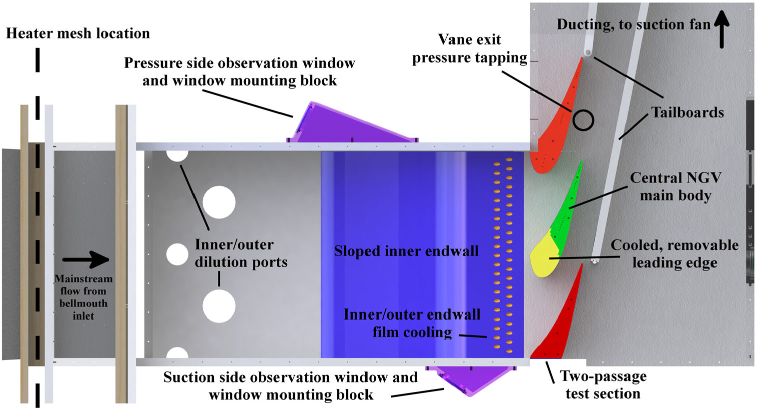
Figure 1. Features of the Oxford Combustor-Turbine Interaction rig.
Butterfly valves and orifice flow meters permit control and measurement of the coolant mass flow rate to the feed plenum of each cooling feature, where the coolant temperature is also measured by a thermocouple. The endwall film cooling is unused in this study, but dilution port and NGV leading edge (LE) film coolant mass flow rates are varied. Only the central vane LE is film-cooled, with the rig being designed to allow this LE to be replaced with various test pieces to allow experiments of different types and on different film hole geometries. The LE film coolant mass flow rate
 ${\dot{{\rm m}}}_{{\rm c}}$
is non-dimensionalised as an average blowing ratio based upon the bulk velocity approaching the vane
${\dot{{\rm m}}}_{{\rm c}}$
is non-dimensionalised as an average blowing ratio based upon the bulk velocity approaching the vane
 $v_{\infty }$
:
$v_{\infty }$
:
 $$M = \frac{{\skew3\dot{m}}_c}{{\rho }_{\infty }v_{\infty }A_h}
\label{eqn4}$$
$$M = \frac{{\skew3\dot{m}}_c}{{\rho }_{\infty }v_{\infty }A_h}
\label{eqn4}$$
where Ah is the combined area of the leading edge film cooling holes and ρ∞ and
 $v_{\infty }$
are the mainstream flow density and velocity, respectively. The dilution port coolant mass flow rate is reported as a momentum flux ratio between the coolant and the mainstream:
$v_{\infty }$
are the mainstream flow density and velocity, respectively. The dilution port coolant mass flow rate is reported as a momentum flux ratio between the coolant and the mainstream:
 $$J_D=\frac{{\rho }_c{v_c}^2}{{\rho }_{\infty }{v_{\infty }}^2}
\label{eqn5}$$
$$J_D=\frac{{\rho }_c{v_c}^2}{{\rho }_{\infty }{v_{\infty }}^2}
\label{eqn5}$$
The combustor-turbine interface plane temperature, turbulence, and velocity profiles at fixed JD = 9 were experimentally measured by Cresci et al.(Reference Cresci, Ireland, Bacic, Tibbott and Rawlinson11,Reference Cresci, Ireland, Bacic, Tibbott and Rawlinson12) . Turbulence intensities were approximately 18% near the midspan and 25% just downstream of the outer endwall film injection. Infrared temperature measurements of the central leading edge are recorded through two Germanium windows positioned to allow observation of both the pressure side (PS) and the suction side (SS). While the coolant-to-mainstream density ratio is not engine-realistic, the leading edge film cooling results are intended for comparison rather than use in engine overall effectiveness calculations etc. Previous research on film cooling density ratio has found that higher density ratios reduce coolant momentum at a given blowing ratio, which tends to reduce jet lift off and thus enhance film effectiveness(Reference Drost and Bölcs13,Reference Pietrzyk, Bogard and Crawford14) . The film effectiveness measurements in this study are therefore expected to be slightly lower than those for equivalent engine condition results. The suction fan speed was kept constant across tests, such that changes to the dilution port and leading edge coolant mass flow rates resulted in a range of Reynolds numbers (based on the vane throat flow properties and chord length) of
 $8.54\times {10}^5$
to
$8.54\times {10}^5$
to
 $1.02\times {10}^6$
. Varying the fan speed while the coolant parameters were fixed at JD = 0 and M = 1.5 showed that across this Reynolds number range the film effectiveness and HTC distributions vary by less than 0.02 and 5%, respectively.
$1.02\times {10}^6$
. Varying the fan speed while the coolant parameters were fixed at JD = 0 and M = 1.5 showed that across this Reynolds number range the film effectiveness and HTC distributions vary by less than 0.02 and 5%, respectively.
2.2 Leading edge test pieces
Three film-cooled, Rohacell foam leading edge test pieces have been investigated in terms of the changes to their film cooling performance across a range of blowing ratios and dilution port mass flow rates. The three models all feature the same cross-sectional profile and identical PS3 and SS3-SS6 hole rows, inclined purely in the streamwise direction. They vary only in terms of the spanwise distribution of radial showerhead hole surface angle, as shown in Fig. 2 (rows PS2-SS2 i.e. the four rows surrounding the geometric stagnation line, which expel coolant in the radial direction of the turbomachine). The position of the geometric stagnation line is also indicated. A fourth foam test piece used in this study features no film cooling holes, but instead includes an array of 42 foil thermocouples distributed over both the PS and SS surfaces. Experiments performed with this ‘calibration test piece’ provided an IR calibration which considered the variation in the magnitude of IR reflections from different locations on the test piece. All test pieces were uniformly spray-painted the same matte black colour in order to minimise the intensity of the reflected radiation originating from the wind tunnel walls.
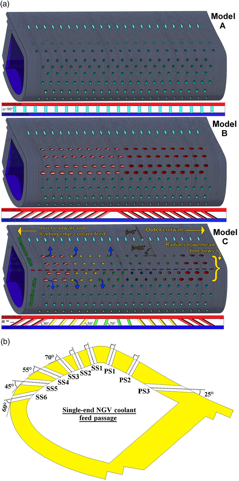
Figure 2. (a) Three film-cooled NGV leading edge geometries and (b) the streamwise inclinations of their hole rows.
2.3 Infrared thermography
Leading edge surface temperatures are acquired simultaneously by two FLIR A655sc infrared cameras at 12.5 frames-per-second throughout the approximately 50 second duration of each heated experiment. This duration is sufficient for the temperatures of both the wind tunnel interior surfaces and the observed test surface to asymptote such that any further changes are less than 1% of the overall local temperature change. For each frame, the surface temperature distribution Ts(x) is calculated according to Equation (6):
 $$T_s({\mathbf x})=\sqrt[4]{\frac{\sigma {T_{bb}({\mathbf x})}^4-(1-\tau )q^*({\mathbf x})}{\sigma \tau \varepsilon }}
\label{eqn6}$$
$$T_s({\mathbf x})=\sqrt[4]{\frac{\sigma {T_{bb}({\mathbf x})}^4-(1-\tau )q^*({\mathbf x})}{\sigma \tau \varepsilon }}
\label{eqn6}$$
where σ is the Stefan-Boltzmann constant. The black-body temperature
 $T_{bb}({\mathbf x})$
is the temperature distribution recorded by the camera on the assumption that all the IR radiation it receives is due to ideal black-body thermal emission from the NGV. In fact, the transmissivity τ of the optical pathway (through the air and Germanium window), the emissivity of the painted vane surface ε, and the extraneous radiation reflecting from the test piece
$T_{bb}({\mathbf x})$
is the temperature distribution recorded by the camera on the assumption that all the IR radiation it receives is due to ideal black-body thermal emission from the NGV. In fact, the transmissivity τ of the optical pathway (through the air and Germanium window), the emissivity of the painted vane surface ε, and the extraneous radiation reflecting from the test piece
 $q^*({\mathbf x})$
must all be accounted for. The product
$q^*({\mathbf x})$
must all be accounted for. The product
 $\tau \varepsilon = \frac{{T_{bb}}^4-{T_{amb}}^4}{{T_w}^4-{T_{amb}}^4}$
was calculated by simultaneously measuring the through-window camera
$\tau \varepsilon = \frac{{T_{bb}}^4-{T_{amb}}^4}{{T_w}^4-{T_{amb}}^4}$
was calculated by simultaneously measuring the through-window camera
 $T_{bb}$
and the observed surface thermocouple temperature
$T_{bb}$
and the observed surface thermocouple temperature
 $T_w$
on a heated aluminium block painted with the same black paint as the Rohacell test pieces, and can be treated as a constant under CTI rig experimental conditions(Reference Holgate, Ireland and Self15). For each heated film cooling experiment performed, a heated experiment with the same rig conditions is also carried out with the calibration test piece. The spatially variant reflection quantity
$T_w$
on a heated aluminium block painted with the same black paint as the Rohacell test pieces, and can be treated as a constant under CTI rig experimental conditions(Reference Holgate, Ireland and Self15). For each heated film cooling experiment performed, a heated experiment with the same rig conditions is also carried out with the calibration test piece. The spatially variant reflection quantity
 $q^*({\mathbf x})$
can then be determined uniquely for each experiment (necessary since it is a function of the rig wall temperatures). It is calculated as the normalised difference between the vane surface radiosity perceived by the IR camera
$q^*({\mathbf x})$
can then be determined uniquely for each experiment (necessary since it is a function of the rig wall temperatures). It is calculated as the normalised difference between the vane surface radiosity perceived by the IR camera
 $\sigma {T_{bb}({\mathbf x})}^{4}$
and the amount of that radiosity which is due to the thermal emissions of the surface
$\sigma {T_{bb}({\mathbf x})}^{4}$
and the amount of that radiosity which is due to the thermal emissions of the surface
 $\sigma \tau \varepsilon {T_w({\mathbf x})}^{4}$
:
$\sigma \tau \varepsilon {T_w({\mathbf x})}^{4}$
:
 $$q^*({\mathbf C}) = \frac{\sigma {T_{bb}}^{4}\left({\mathbf C}\right) - \sigma \tau \varepsilon {T_w}^{4}\left({\mathbf C}\right)}{1-\tau \varepsilon }
\label{eqn7}$$
$$q^*({\mathbf C}) = \frac{\sigma {T_{bb}}^{4}\left({\mathbf C}\right) - \sigma \tau \varepsilon {T_w}^{4}\left({\mathbf C}\right)}{1-\tau \varepsilon }
\label{eqn7}$$
This quantity is calculated separately for each thermocouple location
 ${\mathbf C}$
on the calibration test piece using its temperature reading
${\mathbf C}$
on the calibration test piece using its temperature reading
 $T_w({\mathbf C})$
and the mean
$T_w({\mathbf C})$
and the mean
 $T_{bb}$
value for pixels near to it
$T_{bb}$
value for pixels near to it
 $T_{bb}({\mathbf C})$
. Thermocouple and IR video data are recorded at the same frequency, permitting transient
$T_{bb}({\mathbf C})$
. Thermocouple and IR video data are recorded at the same frequency, permitting transient
 $q^*({\mathbf C})$
measurements. For calculating pixel-wise surface temperatures Ts(x), a pixel-wise
$q^*({\mathbf C})$
measurements. For calculating pixel-wise surface temperatures Ts(x), a pixel-wise
 $q^*({\mathbf x})$
is interpolated from the at-thermocouple values
$q^*({\mathbf x})$
is interpolated from the at-thermocouple values
 $q^*({\mathbf C})$
.
$q^*({\mathbf C})$
.
3.0 EXPERIMENTAL METHODS
3.1 Film effectiveness
A test’s final three seconds of surface temperature data are averaged for calculation of the film effectiveness. By this time, the rig walls and test piece temperatures are essentially steady. Rohacell foam is used for the leading edge test pieces due to its combination of stability under machining and low thermal conductivity (
 $k = 0.032\ {\rm W\ }{{\rm m}}^{-1}{{\rm K}}^{-1}$
). Despite this, the wall thickness between the vane leading edge external surface and the film coolant supply passage is low enough (9 mm) for conduction to produce an appreciable discrepancy between the measured external surface temperature distribution and the corresponding adiabatic wall temperature distribution. Images of the surface temperature on the no-films calibration test piece are used to correct film-cooled surface temperature results for these conduction effects, as detailed by Holgate et al.(Reference Holgate, Ireland and Romero16). The same authors also describe a technique by which the temperature profile generated by the upstream injection of dilution port coolant is removed from the image to yield the true additional cooling effect of the leading edge films.
$k = 0.032\ {\rm W\ }{{\rm m}}^{-1}{{\rm K}}^{-1}$
). Despite this, the wall thickness between the vane leading edge external surface and the film coolant supply passage is low enough (9 mm) for conduction to produce an appreciable discrepancy between the measured external surface temperature distribution and the corresponding adiabatic wall temperature distribution. Images of the surface temperature on the no-films calibration test piece are used to correct film-cooled surface temperature results for these conduction effects, as detailed by Holgate et al.(Reference Holgate, Ireland and Romero16). The same authors also describe a technique by which the temperature profile generated by the upstream injection of dilution port coolant is removed from the image to yield the true additional cooling effect of the leading edge films.
3.2 Heat transfer coefficients
HTCs are determined from the transient phase of the same test used to determine the corresponding film effectiveness at steady-state. They are calculated via a transient, one-dimensional (1D) finite element (FE) conduction model of the test piece wall, implemented in MATLAB. Convective heat transfer boundary conditions are used for both the internal surface (coolant plenum) and the external surface (hot mainstream). The internal driving gas temperature is the NGV coolant temperature
 $T_c$
, which is essentially constant everywhere and throughout an entire test. The internal HTC is estimated as a constant attained with the Dittus-Boelter equation. The results for external HTC were found to have very low sensitivity to the internal HTC, justifying this estimation.
$T_c$
, which is essentially constant everywhere and throughout an entire test. The internal HTC is estimated as a constant attained with the Dittus-Boelter equation. The results for external HTC were found to have very low sensitivity to the internal HTC, justifying this estimation.
The external driving gas temperature history throughout the transient phase
 $T_g({\mathbf x},t)$
can be calculated for each pixel with Equation (8). Since the blowing ratio and coolant-to-mainstream density ratio variations are small throughout the transient (approximately 6% and 10%, respectively), the leading edge coolant jet physics remain essentially unchanged. Therefore, the film effectiveness distribution as determined during the steady-state phase closely approximates the driving gas temperature distribution throughout the transient mainstream temperature rise generated by the heater mesh
$T_g({\mathbf x},t)$
can be calculated for each pixel with Equation (8). Since the blowing ratio and coolant-to-mainstream density ratio variations are small throughout the transient (approximately 6% and 10%, respectively), the leading edge coolant jet physics remain essentially unchanged. Therefore, the film effectiveness distribution as determined during the steady-state phase closely approximates the driving gas temperature distribution throughout the transient mainstream temperature rise generated by the heater mesh
 $T_{\infty }({\textit{t}})$
.
$T_{\infty }({\textit{t}})$
.
 $$T_g({\mathbf x},t) = T_{\infty }(t) - \eta ({\mathbf x}){\mathbf \times }\left(T_{\infty }(t) - T_c\right)
\label{eqn8}$$
$$T_g({\mathbf x},t) = T_{\infty }(t) - \eta ({\mathbf x}){\mathbf \times }\left(T_{\infty }(t) - T_c\right)
\label{eqn8}$$
 $T_{\infty }(t)$
is the mass-averaged temperature of the combustor simulator inlet flow (heated by the heater mesh) and the flow from the dilution ports. When the dilution ports are unused,
$T_{\infty }(t)$
is the mass-averaged temperature of the combustor simulator inlet flow (heated by the heater mesh) and the flow from the dilution ports. When the dilution ports are unused,
 $T_{\infty }(t)$
is just the measured combustor inlet transient temperature. The temperature as measured across the combustor inlet was found to be highly uniform, however the dilution ports create momentum flux ratio-dependent temperature profiles at the cascade inlet. A typical driving gas temperature transient for a single pixel is shown in Fig. 3. The departure from an ideal step rise is caused by initial heat conduction from the mesh into its brass electrical connectors and from the heated flow into the initially ambient temperature rig walls.
$T_{\infty }(t)$
is just the measured combustor inlet transient temperature. The temperature as measured across the combustor inlet was found to be highly uniform, however the dilution ports create momentum flux ratio-dependent temperature profiles at the cascade inlet. A typical driving gas temperature transient for a single pixel is shown in Fig. 3. The departure from an ideal step rise is caused by initial heat conduction from the mesh into its brass electrical connectors and from the heated flow into the initially ambient temperature rig walls.

Figure 3. Iterative progress of the HTC-finding algorithm, showing convergence of FE-predicted surface temperature histories towards the measured history for a single pixel. To reduce the computational requirements of the transient FE calculations, only a reduced, initial portion of the entire heated experiment is considered.
An iterative algorithm was devised to refine an initial pair of HTC guesses
 ${(h_1,h_2)}_0$
at a single pixel for N iterations until the pair of improved guesses
${(h_1,h_2)}_0$
at a single pixel for N iterations until the pair of improved guesses
 ${(h_1,h_2)}_{{\rm N}}$
converges to within a small tolerance. The initial guesses are chosen to span the full range of expected HTC values in the domain, since the algorithm assumes that the true HTC lies somewhere in between. Each HTC guess is applied to the FE model external surface to produce an external surface temperature history prediction
${(h_1,h_2)}_{{\rm N}}$
converges to within a small tolerance. The initial guesses are chosen to span the full range of expected HTC values in the domain, since the algorithm assumes that the true HTC lies somewhere in between. Each HTC guess is applied to the FE model external surface to produce an external surface temperature history prediction
 $T_{s,p}(t)$
intended to resemble the true history
$T_{s,p}(t)$
intended to resemble the true history
 $T_{s,t}(t)$
captured by the camera. A simple error metric E is used to evaluate the closeness of each fit:
$T_{s,t}(t)$
captured by the camera. A simple error metric E is used to evaluate the closeness of each fit:
 $E{\mkern 1mu} = {\mkern 1mu} {\sum _r}\left( {{T_{s,p}} - {T_{s,t}}} \right)$
, where
$E{\mkern 1mu} = {\mkern 1mu} {\sum _r}\left( {{T_{s,p}} - {T_{s,t}}} \right)$
, where
 $\Gamma$
is the set of infrared temperature data points within the time period considered. A positive error metric indicates that
$\Gamma$
is the set of infrared temperature data points within the time period considered. A positive error metric indicates that
 $T_{s,p}(t)$
lies entirely or primarily above
$T_{s,p}(t)$
lies entirely or primarily above
 $T_{s,t}(t)$
and that the associated HTC guess is too high (and vice-versa). The algorithm proceeds as follows at each iteration, and an example of the convergence towards an answer for a single pixel is presented in Fig. 3. The symbols
$T_{s,t}(t)$
and that the associated HTC guess is too high (and vice-versa). The algorithm proceeds as follows at each iteration, and an example of the convergence towards an answer for a single pixel is presented in Fig. 3. The symbols
 $\cap \ $
and
$\cap \ $
and
 $\cup $
refer to logical ‘and’ and ‘or’, respectively.
$\cup $
refer to logical ‘and’ and ‘or’, respectively.
1) For each of the current guesses
${(h_1,h_2)}_n$
perform the FE calculation leading to the predicted surface temperature history.2) Get the error metrics
${(E_1,E_2)}_n$
for the current guesses.3) Determine new guesses
${(h_1,h_2)}_{n+1}$
according to
${(E_1,E_2)}_n$
:
a) If
$(E_{1} > 0\cap E_{2} \lt {\rm{0}})\cup (E_{1} \lt {\rm{0}}\cap E_{2} \gt {\rm{0}})$
i.e. one predicted history lies primarily above and the other primarily below the true history:
$h_{1,n+1}$
- mean of guesses
${(h_1,h_2)}_{{\rm n}}$
$h_{2,n+1}$
- guess
${(h_1,h_2)}_{{\rm n}}$
with the lowest error metric (absolute value)b) If
$(E_{1} > 0\cap E_{2} > 0)$
i.e. both predicted histories lie primarily above the true history:
$h_{{1},n +1 }$
- minimum of guesses
${(h_{1},h_{2})}_n$
$h_{{2},n +1 }$
- minimum of guesses
${(h_{1},h_{2})}_{n-{1}}$
c) If
$(E_{1} \lt 0\cap E_{2} \lt 0)$


i.e. both predicted histories lie primarily below the true history:
 ${h}_{{1},n +1 }$
- maximum of guesses
${h}_{{1},n +1 }$
- maximum of guesses
 ${(h_{1},h_{2})}_n$
 $h_{{2},n +1 }$
- maximum of guesses
$h_{{2},n +1 }$
- maximum of guesses
 ${\left(h_{1},h_{2}\right)}_{n-{1}}$
4) If
$(h_{1,n+1}-h_{2,n+1})$
is less than the tolerance value, the solution is the mean of guesses
${(h_1,h_2)}_{n+1}$
, otherwise return to step 1 with the updated guesses. A tolerance of 0.5 is used, which is small compared to the overall HTC uncertainty.


This process resembles that used by Coletti et al.(Reference Coletti, Scialanga and Arts17) and later Ryley et al.(Reference Ryley, Mcgilvray and Gillespie18) to determine HTC distributions on ribbed internal cooling geometries. They used a commercial, transient FE code and full-surface temperature data (obtained by IR and TLC, respectively) on their complex, three-dimensional (3D) geometries to iteratively refine initial guesses for full-surface HTC distributions. This was intended to improve upon the constraint of 1D geometry imposed by the common analytical solution in Equation (3), while the present technique employs FE to avoid the analytical solution’s initial temperature and semi-infinite substrate assumptions. It also differs from these past FE applications by being simple to implement without a commercial FE code, and in the technique by which the distribution of transient gas driving temperature is determined from the steady-state film effectiveness measurement, as per Equation (8).
The blower fan used in this experiment to supply coolant increases the temperature of the coolant above atmospheric. Before the heater mesh is turned on, the leading edge test pieces are therefore initially exposed to warmed air inside the coolant plenum and predominantly atmospheric air on the external, film-cooled surface. This creates initial depth-wise temperature gradients inside the leading edge test piece which are modelled at each pixel in the FE HTC calculation as a linear temperature gradient between the two sides. In the present experiment, using the FE model and assuming that the temperature throughout the thickness at each pixel is uniformly equal to that pixel’s initial surface temperature results in HTC over-predictions of up to 7%. Increasing the test surface thickness in the FE model to be essentially semi-infinite further increases this maximum error to over 30%. This illustrates the importance in the present experiment of accounting for the initial temperature gradient and the true thickness of the test pieces.
For the present study, a single workstation was used to run the explicit method, 1D FE calculations in a serial MATLAB implementation. Under these conditions, each full surface pressure side HTC solution takes approximately 30 minutes (around 0.01 seconds per converged pixel solution). While acceptable for most experimental purposes, this duration could be significantly improved upon by optimisation of the finite element method and parallelisation, as well as the choice of computer hardware and software.
3.3 Uncertainty analysis
The combustor inlet velocity uncertainty is calculated according to the uncertainties in the pitot tube velocity equation measurands. The coolant mass flow rate uncertainties are calculated in accordance with the orifice meter uncertainty procedures detailed in European Standard ISO 5167-2. The facility is designed for easy removal and replacement of the central vane’s leading edge, and some leakage from the film coolant plenum around the leading edge test pieces into the mainstream is unavoidable. The leading-edge coolant mass flow rate is therefore assigned an additional 2% uncertainty on the basis of an estimation of the leakage area as a proportion of the total cooling hole area. Coolant mass flow rates are reported as dimensionless quantities dependent on the mainstream velocities near the injection points, and uncertainty is propagated from both coolant and mainstream flow velocities and densities. Since the coolant mass flow rates are controlled with hand-operated valves, there is always a small deviation of the measured nominal quantity from its target value, and these deviations were included in the uncertainty estimates. The resulting maximum percentage uncertainties are approximately 12% for M and 5% for
 $J_D$
.
$J_D$
.
Conduction-corrected film effectiveness uncertainties vary slightly over the PS (0.033 to 0.043) and SS (0.029 to 0.034) and are calculated on the basis of the underlying temperature and mass flow rate measurands. HTC uncertainties were estimated using the perturbation method described by Moffat(Reference Moffat19). The variables driving uncertainty in the HTC calculation procedure were surface temperature, material thermal diffusivity, and surface-gas temperature time error, as well as the film effectiveness, coolant temperature and mainstream temperature used in the calculation of the driving gas temperatures. By far the largest contributors to HTC uncertainty are the surface temperature and the film effectiveness. This is apparent in the maps of uncertainty %δHTC in Fig. 4 for both the PS and SS since they resemble the corresponding maps of effectiveness shown in Figs. 5(a) and 6(a). This leads to uncertainties of approximately 9% to 18% on the PS 10% to 60% on the SS. The lower uncertainties occur near PS and upstream SS film rows and are broadly consistent with uncertainties reported in previous, single-row HTC studies. Regions of high film cooling effectiveness (within and after the final SS rows) exhibit greatly elevated HTC uncertainty because they experience a relatively insignificant temperature rise after the mainstream becomes heated. The HTC uncertainties in these regions could be reduced with a greater mainstream-to-coolant temperature difference. Alternatively, conducting a second test in which the coolant is heated rather than the mainstream would create a longer temperature transient in these regions. The HTC results from this test could then be blended with the existing HTC results farther upstream as per Chambers et al.(Reference Chambers, Gillespie, Ireland and Dailey20) (though the experimental technique would essentially become two-test).

Figure 4. Percentage HTC uncertainties on the PS and SS (model C, M = 3.5, JD = 9). Geometric stagnation line indicated.
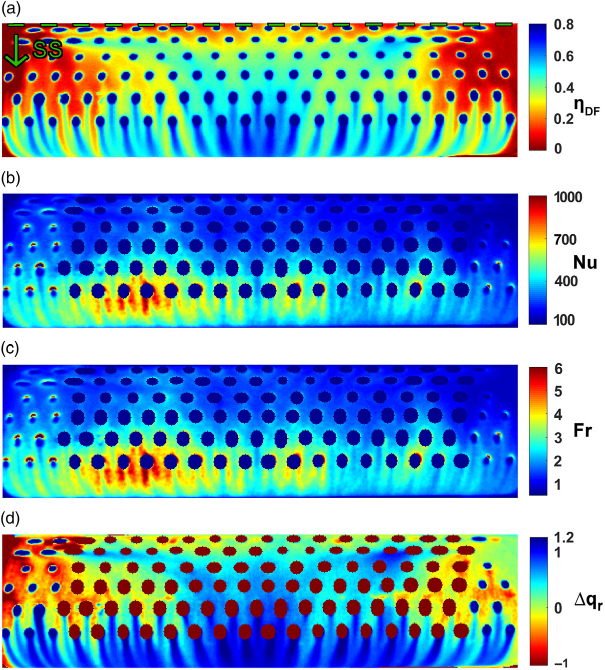
Figure 5. (a) Film effectiveness (b) Nusselt number (c) Frossling number and (d) predicted net heat flux reduction on the suction side (model C, M = 3.5, JD = 9). Geometric stagnation line indicated.
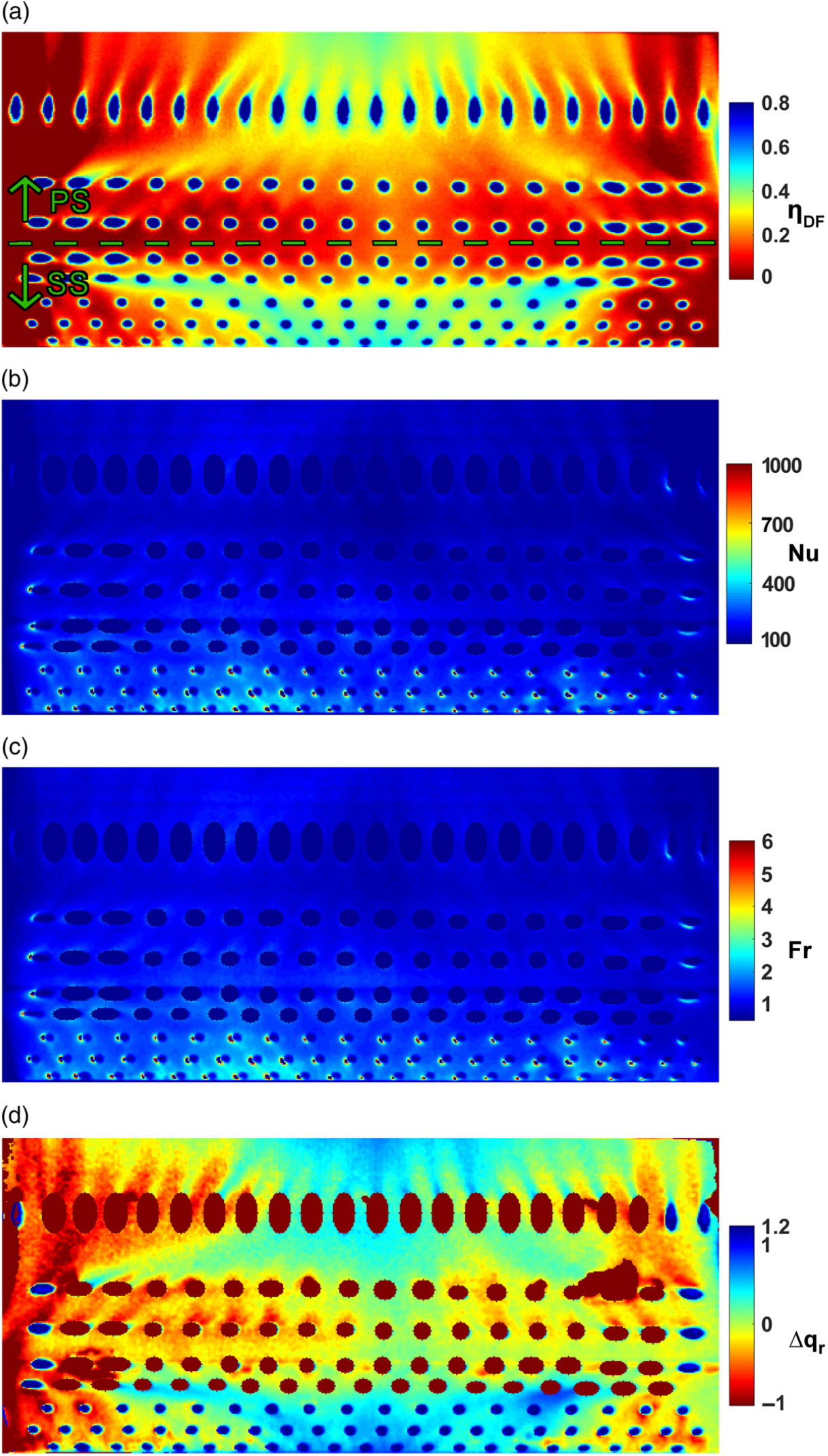
Figure 6. (a) Film effectiveness (b) Nusselt number (c) Frossling number and (d) predicted net heat flux reduction on the pressure side (model C, M = 3.5, JD = 9). Geometric stagnation line indicated.
The 1D FE code was extended to a reduced-domain 3D code in order to assess the influence on HTC results of the 1D conduction assumption. The domains were rectangular prisms comprised of the same number of nodes in the wall thickness direction as in the 1D case, but additional nodes in the surface directions to correspond to the additional surface temperature pixel data available. The pixel for which HTC was calculated remained as the central external surface node, and the unique pixel-wise gas temperature histories calculated according to Equation (8) were applied to their appropriate nodes. The coolant plenum nodes were all subject to the aforementioned convective boundary condition, while the remaining sides of the domain were adiabatic. Regardless of the size of the domain, the results indicated HTC variations consistently less than 2% from the 1D model, justifying the use of the latter. So long as convergence is achieved, the choice of time step makes a negligible difference to results, while the nodal distance used produces results consistently less than 1% different from those produced with smaller distances.
4.0 RESULTS
4.1 Film effectiveness
Figures 5(a) and 6(a) show the SS and PS distributions of film effectiveness on leading edge model C for
 $M=3.5$
and JD = 9. Model C exhibits the most elaborate film effectiveness patterns owing to its varying radial hole surface angles. These results are corrected for 1D conduction effects but not for the temperature profile generated by the dilution ports, making them the effectiveness results relevant for determining the driving gas temperature distribution for HTC calculations. Further detailed distributions of effectiveness have been reported by Holgate et al.(Reference Holgate, Ireland and Romero16,Reference Coletti, Scialanga and Arts17) , with discussion of the effects of dilution port flow on leading edge film cooling performance for various radial showerhead hole inclinations.
$M=3.5$
and JD = 9. Model C exhibits the most elaborate film effectiveness patterns owing to its varying radial hole surface angles. These results are corrected for 1D conduction effects but not for the temperature profile generated by the dilution ports, making them the effectiveness results relevant for determining the driving gas temperature distribution for HTC calculations. Further detailed distributions of effectiveness have been reported by Holgate et al.(Reference Holgate, Ireland and Romero16,Reference Coletti, Scialanga and Arts17) , with discussion of the effects of dilution port flow on leading edge film cooling performance for various radial showerhead hole inclinations.
4.2 Heat transfer coefficients
Heat transfer coefficients are non-dimensionalised as Frossling number according to:
 $$Fr = \frac{Nu}{\sqrt{{Re}_w}} = \frac{h{\rm \ w}}{k_f\sqrt{{Re}_w}}
\label{eqn9}$$
$$Fr = \frac{Nu}{\sqrt{{Re}_w}} = \frac{h{\rm \ w}}{k_f\sqrt{{Re}_w}}
\label{eqn9}$$
Past studies reporting this quantity on cylindrical leading edges used the cylinder diameter as the characteristic length (e.g. Ekkad et al.(Reference Ekkad, Han and Du21), Mick and Mayle(Reference Mick and Mayle22), and Sen et al.(Reference Sen, Schmidt and Bogard23)). By analogy, the vane leading edge axial width w (defined by the axial line segment intersecting both the geometric stagnation point and the suction surface) is used in this study.
 $k_f$
is the fluid thermal conductivity and
$k_f$
is the fluid thermal conductivity and
 ${Re}_w$
is the Reynolds number based on the mainstream approach velocity and characteristic length w. Figures 5(c) and 6(c) show the Frossling number distributions on model C for
${Re}_w$
is the Reynolds number based on the mainstream approach velocity and characteristic length w. Figures 5(c) and 6(c) show the Frossling number distributions on model C for
 $M =3.5$
and JD = 9. Due to convective cooling inside of holes and conduction effects visible in Figs. 5(a) and 6(a), the film effectiveness and hence driving gas temperatures are not accurately known immediately next to each hole exit. Therefore, the hole exits and their immediate surrounds are intentionally excluded from HTC calculation. These near-hole HTCs could be obtained more accurately with a fully 3D FE approach in which appropriate assumptions were made about the convection within the holes. The HTCs are clearly elevated towards the inner endwall (left), especially around SS5 and SS6, due to the slightly higher mainstream velocity generated by the inner endwall contraction(Reference Cresci, Ireland, Bacic, Tibbott and Rawlinson11).
$M =3.5$
and JD = 9. Due to convective cooling inside of holes and conduction effects visible in Figs. 5(a) and 6(a), the film effectiveness and hence driving gas temperatures are not accurately known immediately next to each hole exit. Therefore, the hole exits and their immediate surrounds are intentionally excluded from HTC calculation. These near-hole HTCs could be obtained more accurately with a fully 3D FE approach in which appropriate assumptions were made about the convection within the holes. The HTCs are clearly elevated towards the inner endwall (left), especially around SS5 and SS6, due to the slightly higher mainstream velocity generated by the inner endwall contraction(Reference Cresci, Ireland, Bacic, Tibbott and Rawlinson11).
Figure 7 presents laterally averaged Frossling number for all three models across all three blowing ratios and dilution port momentum flux ratios. Due to the low acceleration on the PS, the HTC is relatively flat, increasing modestly with the elevated mainstream turbulence of higher dilution flow rates and the elevated local turbulence of higher film coolant mass flow rates. SS HTCs increase rapidly as the flow accelerates, producing more turbulence due to increasingly violent shear stresses with subsequent rows of film jets. After the final hole row, the ability of a turbulent boundary layer to grow begins to reduce the HTC. The SS HTCs also tend to increase with higher dilution and film coolant flow rates. Model A tends to produce the highest SS HTCs. Since this model experiences the greatest stagnation region jet lift off and hence the most significant shear and mixing, his suggests a strong dependence of SS HTCs on the turbulence generation by upstream film jets.
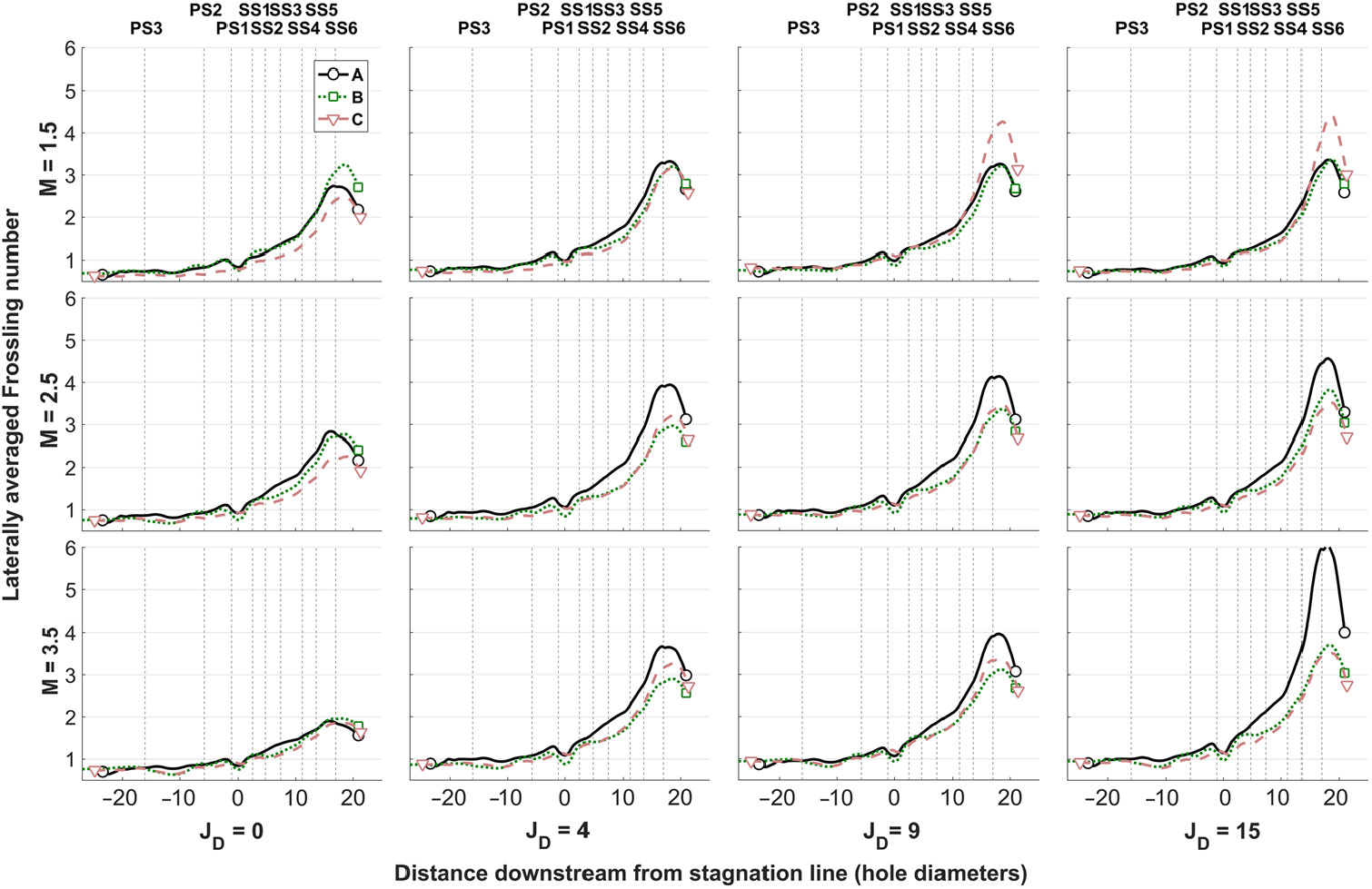
Figure 7. Laterally averaged Frossling number for all three film-cooled leading edge models across three blowing ratios and four dilution port momentum flux ratios.
4.3 Net heat flux reduction
The efficacy of a film cooling design is often assessed with the net surface heat flux reduction
 ${\triangle q}_r$
which would be experienced by an aerofoil under real operating conditions, as defined in Equation (10):
${\triangle q}_r$
which would be experienced by an aerofoil under real operating conditions, as defined in Equation (10):
 $${\triangle q}_r = \frac{q^{\prime\prime}_0 - q^{\prime\prime}_f}{q^{\prime\prime}_0} = 1 - \frac{h_f}{h_0}\left(1-\frac{\eta }{\phi}\right)
\label{eqn10}$$
$${\triangle q}_r = \frac{q^{\prime\prime}_0 - q^{\prime\prime}_f}{q^{\prime\prime}_0} = 1 - \frac{h_f}{h_0}\left(1-\frac{\eta }{\phi}\right)
\label{eqn10}$$
where the subscripts f and 0 indicate quantities with and without film cooling, respectively. The non-dimensionalised surface temperatures
 $\phi=\frac{T_{\infty }-T_s}{T_{\infty }-T_c}$
under such conditions are not available in the present experiment since it neglects the relevant internal cooling features and Biot number. The heat flux reduction is therefore estimated using a common estimate of
$\phi=\frac{T_{\infty }-T_s}{T_{\infty }-T_c}$
under such conditions are not available in the present experiment since it neglects the relevant internal cooling features and Biot number. The heat flux reduction is therefore estimated using a common estimate of
 $\phi =0.6$
(Reference Sen, Schmidt and Bogard23,Reference Mouzon, Terrell, Albert and Bogard24) , while
$\phi =0.6$
(Reference Sen, Schmidt and Bogard23,Reference Mouzon, Terrell, Albert and Bogard24) , while
 $h_0$
is the measurement of HTC on the uncooled calibration test piece. The SS and PS distributions for
$h_0$
is the measurement of HTC on the uncooled calibration test piece. The SS and PS distributions for
 $M =3.5$
and
$M =3.5$
and
 $J_D = 9 $
are shown in Figs. 5(d) and 6(d), respectively. The strong resemblance to the relevant film effectiveness distributions indicates the dominance of effectiveness over HTC in predicting heat fluxes in film cooling scenarios.
$J_D = 9 $
are shown in Figs. 5(d) and 6(d), respectively. The strong resemblance to the relevant film effectiveness distributions indicates the dominance of effectiveness over HTC in predicting heat fluxes in film cooling scenarios.
5.0 CONCLUSIONS
A new technique has been developed for determining both film effectiveness and heat transfer coefficient from a single, heated film cooling experiment. In the steady state phase, experimental film-cooled surface temperature data yield the film effectiveness, which is then used to determine the distribution of driving gas temperatures throughout the transient phase. These are applied to a transient, one-dimensional, finite element model of the test piece material. The pixel-wise solution for heat transfer coefficient is determined by refining guesses until the computationally predicted surface temperature history fits optimally with the experimentally observed one.
The advantages of the technique over conventional analytical techniques are that there is no need to assume that the test piece thickness is essentially semi-infinite or initially uniform in temperature. This increases result accuracy and experimental flexibility, permitting the use of thin-walled test pieces with unequal initial temperatures on the film-cooled and internal surfaces.
The technique was applied to three film-cooled nozzle guide vane leading edge geometries. The model without radial inclination of the four most upstream hole rows experienced higher downstream heat transfer coefficients because of the increased turbulence produced by the upstream jets’ increased penetration into the mainstream. Film effectiveness dominates in predictions of net heat flux reduction due to leading edge film cooling.
ACKNOWLEDGMENTS
This research was supported by Rolls-Royce and the UK Engineering and Physical Sciences Research Council under the Centre for Doctoral Training in Gas Turbine Aerodynamics. The authors are grateful to Mr. David O’Dell and Mr. Trevor Godfrey of the Oxford Thermofluids Institute for manufacturing and instrumenting the test pieces used in this study.


