


1. Introduction
Non-isothermal reactive transport within complicated porous media is widely encountered in energy, environmental science and engineering applications, including natural subsurface smouldering fires (Rein Reference Rein2009; Mokheimer et al. Reference Mokheimer, Hamdy, Abubakar, Shakeel, Habib and Mahmoud2019), smouldering remediation of coal-tar-contaminated soil (Scholes et al. Reference Scholes, Gerhard, Grant, Major, Vidumsky, Switzer and Torero2015), underground coal gasification for coal mining (Bhutto, Bazmi & Zahedi Reference Bhutto, Bazmi and Zahedi2013) and in situ combustion (ISC) for crude oil recovery (Mahinpey, Ambalae & Asghari Reference Mahinpey, Ambalae and Asghari2007). The temperature-dependent chemical reaction rate and transport properties enhance the nonlinear nature of reactive transport. For example, during the ISC process, high-pressure air is injected into the reservoir and reacts with the solid residue formed from thermal/oxidative pyrolysis of the crude oil, referred to as coke, to release combustion heat (Mahinpey et al. Reference Mahinpey, Ambalae and Asghari2007). The combustion front propagates through the reservoir and displaces the heavy oil downstream into the production well and improves oil mobility heating by coke combustion, averaging 773–1173 K (Liang et al. Reference Liang, Guan, Wu, Wang and Huang2013; Mokheimer et al. Reference Mokheimer, Hamdy, Abubakar, Shakeel, Habib and Mahmoud2019). However, unreasonable operating conditions for specified reservoir conditions, including the ignition temperature and air injection rate (Moore et al. Reference Moore, Laureshen, Mehta and Ursenbach1999; Liu et al. Reference Liu, Tang, Zheng and Song2021), may induce combustion instabilities, such as combustion extinction with a low burning temperature, flaming combustion with an extremely high burning temperature and air breakthrough into the production well (Liang et al. Reference Liang, Guan, Jiang, Xi, Wang and Li2012). A deep understanding of the non-isothermal reactive flow at the combustion front is essential to achieve a successful ISC project with sustained combustion front propagation.
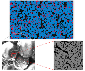
At the combustion front shown in figure 1, coke combustion is coupled with weakly compressible gas flow, species transport, conjugate heat transfer and heterogeneous coke oxidation kinetics in a complex coked porous medium (Xu et al. Reference Xu, Long, Jiang, Zan, Huang, Chen and Shi2018b; Lei, Wang & Luo Reference Lei, Wang and Luo2021). Furthermore, the geometrical structure continually evolves as the coke burns out into gas products, thereby changing the heat and mass transport properties of the channels and their surroundings. The pores in the coked porous medium can be categorized as micrometre-range pores  $({\sim} O(1)\;\mathrm{\mu }\textrm{m)}$ in the rock void space and nanometre-range pores
  $({\sim} O(10)\;\textrm{n}\textrm{m)}$ in the coke void space. Commonly, the micrometre-range pores can be resolved by X-ray computed micro-tomography (micro-CT) images (Xu et al. Reference Xu, Long, Jiang, Ma, Zan, Ma and Shi2018a), referred to hereafter as the resolved macropores, while the nanometre-range pores are below the image resolution, referred to hereafter as the unresolved (sub-resolution) nanopores. Nanoscale refined pores introduce different flow regimes and then Knudsen diffusion primarily occurs at the sub-resolution nanopores. The complex nonlinear nature of the multiple physicochemical and thermal processes in multiscale porous media increases the complications compared with isothermal reactive flow problems in stationary porous media. Considerable experimental and numerical studies have been carried out to explore the effect of operating conditions on combustion dynamics (Aleksandrov, Kudryavtsev & Hascakir Reference Aleksandrov, Kudryavtsev and Hascakir2017; Zhu et al. Reference Zhu, Liu, Liu, Wang and Kovscek2019; Yuan et al. Reference Yuan, Sadikov, Varfolomeev, Khaliullin, Pu, Al-Muntaser and Saeed Mehrabi-Kalajahi2020; Liu et al. Reference Liu, Tang, Zheng and Song2021). Among the experimental work, one-dimensional combustion tube experiments were performed to guide the operating conditions at the ISC field project. However, the inconsistent thermal conditions between laboratory investigations and reservoir conditions, such as the high heat capacity of the experimental apparatus designed for elevated temperature and pressure, and the imperfect thermal insulation system designed for adiabatic boundaries, result in conventional combustion tube experiments that cannot operate at low air fluxes to establish stable combustion front propagation (Alamatsaz et al. Reference Alamatsaz, Moore, Mehta and Ursenbach2011). Therefore, the air flux in combustion tube experiments, averaging 30 sm3 (air) (m2 h)−1, is significantly greater than the air flux experienced in the field, where the minimum air flux can be 0.55 sm3 (air) (m2 h)−1 (Moore et al. Reference Moore, Laureshen, Mehta and Ursenbach1999). Regarding unscaled air fluxes, there remains significant concern about whether sustainable combustion can be reproduced in field applications when given the feasible operating parameters from experimental studies. Moreover, high-temperature and high-pressure experiments pose great challenges in revealing the fundamental combustion dynamics regime behind fully coupled thermal and reactive processes (Aleksandrov et al. Reference Aleksandrov, Kudryavtsev and Hascakir2017; Yuan et al. Reference Yuan, Sadikov, Varfolomeev, Khaliullin, Pu, Al-Muntaser and Saeed Mehrabi-Kalajahi2020).

Figure 1. General representation of coke combustion in the multiscale porous medium with pore space in different characteristic length: the resolved macropores surrounded by the rock grains and unresolved nanoporous continuum in the coke regions.
Regarding numerical simulations, most existing numerical studies (Cinar, Castanier & Kovscek Reference Cinar, Castanier and Kovscek2011; Nissen et al. Reference Nissen, Zhu, Kovscek, Castanier and Gerritsen2015; Liu et al. Reference Liu, Tang, Zheng and Song2021) employ macroscopic or representative element volume (REV) solutions, which simulate coke combustion in porous media using volume-averaged geometrical properties, transport properties and the coke combustion rate. Without explicit pore-scale details, the REV-based or Darcy-scaled model often filters the flow instability with preferential penetration related to the local geometry (Lei & Luo Reference Lei and Luo2021). Furthermore, the volume-averaged chemical reaction rate is highly nonlinear owing to the effective reaction rate being a complex function of the specific surface area, local advection-diffusion conditions and intrinsic reaction rate determined by the local thermodynamic conditions (Molins Reference Molins2015; Soulaine et al. Reference Soulaine, Roman, Kovscek and Tchelepi2017; Xu et al. Reference Xu, Long, Jiang, Zan, Huang, Chen and Shi2018b; Yang et al. Reference Yang, Dai, Xu, Liu, Zan, Long and Shi2021a). The challenges of REV-scale closure problems remain for obtaining an effective reaction rate (or mass exchange coefficients), effective transport properties and effective geometrical properties (Golfier et al. Reference Golfier, Bazin, Lenormand and Quintard2004). Compared with the chemical rate under isothermal conditions, the intrinsic coke combustion rate is highly sensitive to the local temperature, making upscaling of those effective properties to be more sophisticated. Therefore, the highly nonlinear nature of different coke combustion regimes makes it practically impossible to understand the mechanism based on the REV-based solution.
Recently, pore-scale modelling of reactive flow has attracted growing interest to provide deeper insight into the physics of reactive flow in complicated porous media (Rein Reference Rein2009; Qiu et al. Reference Qiu, Dennison, Knehr, Kumbur and Sun2012; Pereira Nunes, Blunt & Bijeljic Reference Pereira Nunes, Blunt and Bijeljic2016; Soulaine et al. Reference Soulaine, Roman, Kovscek and Tchelepi2017, Reference Soulaine, Roman, Kovscek and Tchelepi2018; Soulaine, Creux & Tchelepi Reference Soulaine, Creux and Tchelepi2019; Maggiolo et al. Reference Maggiolo, Picano, Zanini, Carmignato, Guarnieri, Sasic and Ström2020), particularly with the accelerating development of imaging techniques (Bultreys, De Boever & Cnudde Reference Bultreys, De Boever and Cnudde2016) and well-established image processing techniques. Regarding the pore-scale modelling of the combustion front during ISC processes, several attempts have been conducted over the past five years. Xu et al. (Reference Xu, Long, Jiang, Ma, Zan, Ma and Shi2018a) reconstructed micro-CT images of coked packed beds with 500 nm pixel resolution and found that the basic coke deposition pattern was pore filling in narrow pore throats. Based on three-dimensional (3-D) digital rock, single-phase flow and mass diffusion processes were simulated to quantify the effect of coke deposition on the permeability and mass diffusivity, respectively (Xu et al. Reference Xu, Long, Jiang, Ma, Zan, Ma and Shi2018a). However, few studies that are directly based on micro-CT images have been developed to model coke combustion in realistic coked porous structures. Regarding the coke combustion simulation, Xu et al. (Reference Xu, Long, Jiang, Zan, Huang, Chen and Shi2018b) was one of the first to develop a single-relaxation-time (SRT) lattice Boltzmann (LB) model to simulate coke combustion in an ideal and small computational domain meshed in 100 × 480 cells. Lei et al. (Reference Lei, Wang and Luo2021) developed a multiple-relaxation-time (MRT)-LB model instead of the SRT-LB model to improve the numerical accuracy and stabilities. They also included the equation of state for an ideal gas to diminish the constant density assumption that accounts for the thermal expansion effect on coke combustion. These studies (Xu et al. Reference Xu, Long, Jiang, Zan, Huang, Chen and Shi2018b; Lei et al. Reference Lei, Wang and Luo2021) extended our knowledge of coke combustion dynamics and influencing factors during ISC processes, although some limitations in the numerical model still exist. First, the one-way coupling between the coke combustion reaction and the weakly compressible gas flow was made without considering the effect of the dramatic gas production on mass transfer. Second, the energy conversion law broke down when using the volume of pixel (VOP) method (Kang, Lichtner & Zhang Reference Kang, Lichtner and Zhang2006) to handle the temporal evolution of the coke phase in a binary manner for the non-isothermal reactive flow. Third, the computation domain remained restricted to the ideal porous medium consisting of staggered or random arrangements of circle-like grains with all coke deposited on the grain surface (Xu et al. Reference Xu, Long, Jiang, Zan, Huang, Chen and Shi2018b; Lei & Luo Reference Lei and Luo2021). However, the effect of realistic coke deposition on coke combustion was not explored, including the pore-filling deposition pattern and the multiscale nature. Fourth, coke naturally deposits in pore throats and blocks most of the connectable pathways (Xu et al. Reference Xu, Long, Jiang, Ma, Zan, Ma and Shi2018a). However, the previous LB model for idealized porous structures typically considered coke to be an impermeable obstacle regardless of the gas flow through the coke nanopores (Xu et al. Reference Xu, Long, Jiang, Zan, Huang, Chen and Shi2018b; Lei & Luo Reference Lei and Luo2021), which led to the simulation of coke combustion through a multiscale coked porous medium to be difficult or even impossible to perform. Fifth, only the coke combustion reaction that occurred on the external sharp reactive interface between the coke and fluid grid cell was considered without accounting for the internal sub-resolution nanopores (Bhatia & Perlmutter Reference Bhatia and Perlmutter1980) and the Knudsen diffusion through the coke nanopores (Fong, Jorgensen & Singer Reference Fong, Jorgensen and Singer2018). This may introduce inhibited reactivity, leading to varied combustion regimes. Considering the imaging resolution and unacceptable computation cost, direct ‘pore’-scale modelling of the coke combustion dynamics for the multiscale pores is practically impossible. Therefore, multiscale pore-scale modelling of the coupled thermal and reactive flow still must be developed to improve mass and energy conservation during the evolution of the pore-filling coke structure with combustion.
An elegant idea to model multiscale phenomena is hybrid modelling (Neale & Nader Reference Neale and Nader1974; Golfier et al. Reference Golfier, Zarcone, Bazin, Lenormand, Lasseux and Quintard2002, Reference Golfier, Bazin, Lenormand and Quintard2004; Luo et al. Reference Luo, Quintard, Debenest and Laouafa2012, Reference Luo, Laouafa, Guo and Quintard2014, Reference Luo, Laouafa, Debenest and Quintard2015), which describes the fluid dynamics in the larger channel using the Navier–Stokes equation while modelling the flow through the surrounding porous medium by the Darcy law. This idea dates back to the work of Brinkmann (Reference Brinkman1949b), who proposed the Darcy–Brinkmann–Stokes (DBS) equation with the combination of the Brinkmann term and the Darcy law for the flow in a high-porosity porous medium. The DBS equation was also validated for both flows in the larger channels and the matrix (Neale & Nader Reference Neale and Nader1974; Whitaker Reference Whitaker1986). Golfier et al. (Reference Golfier, Zarcone, Bazin, Lenormand, Lasseux and Quintard2002) employed the DBS equation to simulate heterogeneous mineral dissolution in both the fluid and porous regions with a local non-equilibrium dissociation condition. Unlike these Darcy-scale simulations (Golfier et al. Reference Golfier, Zarcone, Bazin, Lenormand, Lasseux and Quintard2002, Reference Golfier, Bazin, Lenormand and Quintard2004) Soulaine et al. (Soulaine & Tchelepi Reference Soulaine and Tchelepi2016; Soulaine et al. Reference Soulaine, Roman, Kovscek and Tchelepi2017) employed pore-scale models based on the DBS approach, which introduced bounding values of the local porosity  ${\varepsilon _f} = 1$ and
  ${\varepsilon _f} = 0 \equiv 0.01$ to represent the resolved macropores and the impermeable rocks in images and intermediate
  $0 < {\varepsilon _f} < 1$ to represent the unresolved pores. Such hybrid modelling of the fluid flow with a single DBS equation was regarded as the micro-continuum DBS approach (Soulaine & Tchelepi Reference Soulaine and Tchelepi2016; Soulaine et al. Reference Soulaine, Roman, Kovscek and Tchelepi2017). Their studies (Soulaine & Tchelepi Reference Soulaine and Tchelepi2016; Soulaine et al. Reference Soulaine, Roman, Kovscek and Tchelepi2017) showed that the pore-scale micro-continuum framework can efficiently bridge the gap between modelling of the resolved and unresolved pores in the images. For the image-based single-phase fluid flow simulation, the pore-scale micro-continuum model can be used to solve for the standard Navier–Stokes flow in the resolved macropore channels, degenerate to Darcy laws in the unresolved nanopore regions, reproduce the non-slip velocity condition at the macropore-rock interface by penalization, and ensure continuity of the stress and velocity in the entire computational domain (Soulaine & Tchelepi Reference Soulaine and Tchelepi2016). With the appealing micro-continuum framework, mineral dissolution and wormholes were simulated by Soulaine et al. (Reference Soulaine, Roman, Kovscek and Tchelepi2017) in micromodel pore networks to observe five different dissolution regimes. Scheibe et al. (Reference Scheibe, Perkins, Richmond, McKinley, Romero-Gomez, Oostrom, Wietsma, Serkowski and Zachara2015) applied the DBS equation to simulate the flow and transport in 3-D micro-CT images with unresolved pores for better agreement with the experimental results. Recently, the micro-continuum framework was further extended to model multiphase flow in a multiscale porous medium (Carrillo, Bourg & Soulaine Reference Carrillo, Bourg and Soulaine2020). Soulaine et al. investigated pore-scale multiphase reactive transport in mineral dissolution with CO2 production (Soulaine et al. Reference Soulaine, Roman, Kovscek and Tchelepi2018) and shale formation (Soulaine et al. Reference Soulaine, Creux and Tchelepi2019) for deeper insight into the mechanisms behind such multiscale transport phenomena. To date, these multiscale pore-scale modelling efforts on reactive flow have focused on isothermal processes in the presence of sharp reactive interfaces. To the best of our knowledge, few studies have been devoted to the more nonlinear dynamics of non-isothermal reactive flow accompanied by rich reactive nanopore surfaces within the sub-resolution matrix and their structural evolution with chemical reactions, such as coke combustion during ISC processes.
The present study extends the pore-scale micro-continuum model to non-isothermal reactive flow through a multiscale porous medium in the presence of unresolved reactive nanopores. The single-phase model was introduced to account for the coke combustion between the solid fuel and the high-pressurized gaseous air, because the mobilizing oil, liquid water and light hydrocarbon gas have been vaporized/transported downstream of the combustion zone. Particular attention is given to sub-grid models for reactive transport that occur in the sub-resolution nanopores of the segmented coke phase, including Knudsen diffusion and the reactive surface area. The present study revisits the previous coke combustion problem (Xu et al. Reference Xu, Long, Jiang, Zan, Huang, Chen and Shi2018b) to demonstrate the improvements of the developed micro-continuum model, such as improved energy conservation during geometrical evolution. Furthermore, image-based coke combustion is simulated to investigate the effect of the multiscale porous medium on coke combustion and highlight the significance of sub-grid reactive transfer. The effects of ignition temperature and air flux are investigated to explore the five combustion dynamics regimes for the homogeneous base porous medium with different combustion characteristics in terms of combustion temperature and combustion front morphological pattern. Additionally, the study provides insights into the different combustion regimes that emerge in typical experimental and field operations, as well as risk control for sustainable combustion.
This paper is organized as follows. In § 2, a computational domain based on micro-CT images, governing equations for the coupled non-isothermal reactive flow and sub-grid reactive transfer models are introduced. In § 3, the numerical algorithm developed to solve the nonlinear problem with the open-source simulation platform OpenFOAM is described with more details in Appendix A. The validation and improvement analyses are given with some details in Appendix B and the supplementary material. The grid convergence test is shown in Appendix C. In § 4, the combustion regimes with different combustion characteristics and the effects of air flux and ignition temperature are analysed. We close with a summary and conclusion.
2. Mathematical and physical models
2.1. Pore-scale domain with realistic coke deposition pattern
Coke combustion was investigated in a two-dimensional (2-D) pore-scale computational domain constructed from micro-tomographic images by micro-CT (nanoVoxel-3000) for the coked porous media. The micro-CT system built digital images of 1700 × 1700 × 2100 voxels with a voxel resolution of 500 nm. A 2-D slice consisting of 1200 × 2000 voxels (dimensions 0.6 × 1 mm2) or 2.4 million grid cells, shown in figure 2(a), was cropped from the reconstructed data and imported into the ilastik toolkit (Berg et al. Reference Berg2019) for image segmentation by machine learning algorithms. The image segmentation workflow began from label assignments of the coke, rock and pore pixels through human annotations drawn on the raw greyscale image. Random forest classifiers were trained to learn the labelled features and empower the prediction capacity to partition the image into the coke, rock and pore phases. The labelling–training–prediction workflow was looped in an interactive mode to correct the classification flaw until the desired segmentation was achieved, as illustrated in figure 2(b). After segmentation, the volume fraction of the pore pixels was 23.8 %, while the coke volume fraction was 8.19 %. For the present coke combustion simulation, two additional open flow buffer regions 20 pixels wide were added before and after the entrance of the coked porous medium so that the fully developed boundary condition could be enforced at the inlet and outlet boundaries of the computational domain.

Figure 2. (a) Two-dimensional raw image slice scanned by micro-CT showing rock grains (lightest grey), coke (grey) and pore (darkest grey) and (b) segmented image slice for computational domain with coloured phase of interest for rock grains (blue), coke (red) and pore (black).
As observed in figure 2(b), the base matrix was packed with an idealized sphere-like glass bead pack, regarded as the sandstone proxy. Coke tended to deposit inside the pore throat, which agrees with previous observations from scanning electron microscopy (Xu et al. Reference Xu, Long, Jiang, Ma, Zan, Ma and Shi2018a). The coke deposition pattern blocked all of the connectable pore network if the coke was considered an impermeable obstacle. This implied that the previous numerical method (Xu et al. Reference Xu, Long, Jiang, Ma, Zan, Ma and Shi2018a), which neglected the effect of the sub-resolution continuum on the fluid flow, is not suitable for modelling the reactive flow in such a realistic coked porous medium. Additionally, the non-uniform spatial distribution of the coke deposition resulted in coke accumulations that were rich in some local regions but poor in other regions, increasing the heterogeneity of the coked porous medium. The naturally heterogeneous coke deposition in pore throats showed a significant difference compared with the previous idealized structures (Xu et al. Reference Xu, Long, Jiang, Zan, Huang, Chen and Shi2018b; Lei et al. Reference Lei, Wang and Luo2021), which were composed of staggered or random arrangements of circle-like grains with all coke deposited on the grain surface.
2.2. Governing equation and assumptions
The micro-CT system with micrometre-scale resolution and millimetre-scale field of view cannot resolve the pore structure in coke regions because the characteristic length scales of the coke nanopores and the rock macropores differ by orders of magnitudes. In addition, the direct pore-scale simulation for all the scales is unacceptable owing to the enormous computational cost for billion-cell representations despite the 2-D simulation problems. Therefore, the multiscale modelling framework (i.e. the micro-continuum approach for pore-scale simulation) was introduced to establish the governing equations for the multiscale coke combustion dynamics. With the micro-continuum approach, structured Cartesian-type grid cells directly correspond to the voxel elements of the segmented image in figure 2(b) without requiring a complex mesh technique. The volume fraction of void space in each grid cell,  ${\varepsilon _f}$, referred to as the local porosity, was imposed to represent the complex multiscale pore structure and filter the explicit structural information below the micro-CT resolution limit. In the current filtering strategy, the pore regions labelled in the segmented image were denoted by
  ${\varepsilon _f} = 1$ to represent the clear fluid zone, while the rock regions were denoted by
  ${\varepsilon _f} = 0$ to represent impermeable solid zones without small pore space. For the coke regions, an intermediate value of
  $0 < {\varepsilon _f} < 1$ can be given to symbolize the sub-resolution porous medium with an aggregate of nanopores and coke solids, as shown in figure 1. The intermediate value is equal to the intrinsic coke porosity, which depends on coke formation conditions, such as crude oil properties and pyrolysis temperature. In the present study, the sub-resolution coke porosity was specified as 0.7 to account for the gas transport and chemical reactions in such porous coke structures. The grid cells were assumed to not contain both the rock and the coke; therefore, the volume fraction of the rock phase,
  ${\varepsilon _{rock}}$, or the volume fraction of the coke phase,
  ${\varepsilon _{coke}}$, can be derived according to the known values of
  ${\varepsilon _f}$ and the constraint relation as
 \begin{equation}{\varepsilon _f} + {\varepsilon _{coke}} + {\varepsilon _{rock}} = 1.\end{equation}
In the micro-continuum approach, partial differential equations (PDEs) are averaged over control volumes, corresponding to the grid cells, to govern the conservation law of energy, mass and species concentrations, which are modelled with averaged field variables. According to the volume averaging theory, these PDEs hold for all computational cells regardless of their contents. Before deriving the governing equations, the following assumptions were made to simplify the modelling of the complex hybrid-scale physics:
(1) the non-slip boundary condition is held at the impermeable rock interface owing to the approximated Knudsen number of 2.28 × 10⁻³ in the resolved macropores surrounded by the rock grains;
(2) the heat capacities of the gas and solid components are constant and only depend on the initial temperature and pressure (Lei et al. Reference Lei, Wang and Luo2021);
(3) the densities of the solid components are constant;
(4) the gas is an ideal gas with the equation of state as (2.2)
(2.2) \begin{equation}{\rho _f} = {\bar{p}_f}/R\bar{T},\end{equation}

where  ${\bar{p}_f}$ is the intrinsically phase averaged pressure,
  ${\bar{p}_f} = (1/{V_f})\int_{{V_f}} {{p_f}} \,\textrm{d}V$;
(5) the radiative heat transfer is not considered;
(6) the thermal equilibrium condition is valid within each coke cell at 500 nm resolution when the burning temperature is less than 1200 K, which maintains
(2.3)\begin{equation}\varUpsilon = \frac{{\left|{\frac{{\dot{r}{h_r}}}{{\rho {c_p}}}} \right|}}{{\left|{\alpha \frac{{{\partial^2}T}}{{\partial {x^2}}}} \right|}} = O\left( {\frac{{\dot{r}{h_r}{L^2}}}{{\rho {c_p}\alpha T}}} \right) \ll 1,\end{equation}

where  $\varUpsilon$ is the ratio of the reaction term and the thermal conductive term in the energy equation, hr is the coke combustion heat,
  $\dot{r}$ is the coke combustion rate, and L is the cell size, 500 nm;
(7) the coke combustion is modelled as (2.4), which indicates that the coke reacts with the oxygen in the injected hot air to produce CO2. The reaction rate is estimated according to a first-order Arrhenius equation as (2.5)
(2.4)\begin{gather}\textrm{C} + {\textrm{O}_\textrm{2}} \to \textrm{C}{\textrm{O}_\textrm{2}} + {h_r},\end{gather}(2.5)\begin{gather}\dot{r} = {a_v}Aexp \left( { - \frac{E}{{R\bar{T}}}} \right)\frac{{{\rho _f}{{\bar{\omega }}_{f\textrm{,}{\textrm{O}_\textrm{2}}}}}}{{{M_{{\textrm{O}_\textrm{2}}}}}},\end{gather}


where  ${a_v}$ is the reactive surface area per control volume, which is only non-zero at the grid cells containing the coke. The detailed sub-grid model of the reactive surface area will be discussed in § 2.3. In the coke combustion kinetics formulation, A and E are the pre-exponential factor and activation energy, respectively, while R is the ideal gas constant,
  ${\rho _f}$ is the gas density, and
  ${M_{{\textrm{O}_\textrm{2}}}}$ is the molecular weight of the oxygen. To match the following volume averaging governing equations,
  $\bar{T}$ represents the temperature averaged over the control volume,
  $\bar{T} = (1/V)\int_V T \,\textrm{d}V$, and
  ${\bar{\omega }_{f\textrm{,}{\textrm{O}_\textrm{2}}}}$ is the O2 mass fraction intrinsically averaged over the gas phase,
  ${\bar{\omega }_{f\textrm{,}{\textrm{O}_\textrm{2}}}} = (1/{V_f})\int_{{V_f}} {{\omega _{f\textrm{,}{\textrm{O}_\textrm{2}}}}} \,\textrm{d}V$. In this simulation, the coke combustion kinetics of A, E and hr are set as
  $9.717 \times {10^6}\;\textrm{m}\;{\textrm{s}^{ - 1}}$, 131.09 kJ mol−1 and 388.5 kJ mol−1, respectively (Ren, Freitag & Mahinpey Reference Ren, Freitag and Mahinpey2007), which are the same values as in previous studies (Xu et al. Reference Xu, Long, Jiang, Zan, Huang, Chen and Shi2018b; Lei et al. Reference Lei, Wang and Luo2021) for better comparisons of different numerical models.
According to the above analysis and assumptions, a set of the volume averaging governing equations for multiscale coke combustion are shown in (2.6)–(2.10), which are valid throughout the domain regardless of the content of the grid cell:
 \begin{gather}\frac{1}{{{\varepsilon _f}}}\left( {\frac{{\partial {\rho_f}\bar{\boldsymbol{U}}}}{{\partial t}}+ \boldsymbol{\nabla }\boldsymbol{\cdot }\left( {\frac{{{\rho_f}}}{{{\varepsilon_f}}}\boldsymbol{\bar{U}\bar{U}}} \right)} \right) ={-} \boldsymbol{\nabla }{\bar{p}_f} + {\rho _f}g + \frac{{{\mu _f}}}{{{\varepsilon _f}}}{\nabla ^2}\bar{\boldsymbol{U}} - {\mu _f}{k^{ - 1}}\bar{\boldsymbol{U}},\end{gather}
 \begin{gather}\frac{{\partial {\rho _f}{\varepsilon _f}}}{{\partial t}} + \boldsymbol{\nabla }\boldsymbol{\cdot }({\rho _f}\bar{\boldsymbol{U}}) ={-} {\dot{m}_{coke}},\end{gather}
 \begin{gather}\frac{{\partial {\rho _{coke}}{\varepsilon _{coke}}}}{{\partial t}} = {\dot{m}_{coke}},\end{gather}
 \begin{gather}\frac{{\partial {\varepsilon _f}{\rho _f}{{\bar{\omega }}_{f,i}}}}{{\partial t}} + \boldsymbol{\nabla }\boldsymbol{\cdot }({\rho _f}\boldsymbol{U}{\bar{\omega }_{f,i}}) = \boldsymbol{\nabla }\boldsymbol{\cdot }({\varepsilon _f}{\rho _f}{\hat{D}_{i,eff}}\boldsymbol{\nabla }{\bar{\omega }_{f,i}}) + {\dot{m}_i},\quad i = {\textrm{O}_\textrm{2}}\textrm{,C}{\textrm{O}_\textrm{2}},\end{gather}
 \begin{gather}\dfrac{{\partial
{\varepsilon _s}{\rho _s}{h_s}}}{{\partial t}} +
\dfrac{{\partial {\varepsilon _f}{\rho _f}{h_f}}}{{\partial
t}} + \boldsymbol{\nabla }\boldsymbol{\cdot }({\rho
_f}\bar{\boldsymbol{U}}{h_f}) + \dfrac{{\partial {\rho
_f}K}}{{\partial t}} + \boldsymbol{\nabla
}\boldsymbol{\cdot }({\rho
_f}\bar{\boldsymbol{U}}K)\nonumber\\
\qquad=
\dfrac{{\partial {{\bar{p}}_f}}}{{\partial t}} +
\boldsymbol{\nabla }\boldsymbol{\cdot }({\lambda
_{eff}}\boldsymbol{\nabla }T) + {\rho
_f}\bar{\boldsymbol{U}}\boldsymbol{\cdot }\boldsymbol{g} +
{{\dot{q}}_r}.\end{gather}
\begin{gather}\dfrac{{\partial
{\varepsilon _s}{\rho _s}{h_s}}}{{\partial t}} +
\dfrac{{\partial {\varepsilon _f}{\rho _f}{h_f}}}{{\partial
t}} + \boldsymbol{\nabla }\boldsymbol{\cdot }({\rho
_f}\bar{\boldsymbol{U}}{h_f}) + \dfrac{{\partial {\rho
_f}K}}{{\partial t}} + \boldsymbol{\nabla
}\boldsymbol{\cdot }({\rho
_f}\bar{\boldsymbol{U}}K)\nonumber\\
\qquad=
\dfrac{{\partial {{\bar{p}}_f}}}{{\partial t}} +
\boldsymbol{\nabla }\boldsymbol{\cdot }({\lambda
_{eff}}\boldsymbol{\nabla }T) + {\rho
_f}\bar{\boldsymbol{U}}\boldsymbol{\cdot }\boldsymbol{g} +
{{\dot{q}}_r}.\end{gather}
The momentum conservation equation, known as the DBS equation (Brinkman Reference Brinkman1949a), is expressed in (2.6), where  $\bar{\boldsymbol{U}}$ is the superficial velocity, namely, the Darcy velocity, t is the time, g is the gravitational acceleration and
  ${\mu _f}$ is the gas viscosity. The k −1 in the last term of the (2.6) is the reciprocal of the absolute permeability, which varies with the local porosity via the commonly used Kozeny–Carman equation:
 \begin{equation}{k^{ - 1}} = k_0^{ - 1}\frac{{{{(1 - {\varepsilon _f})}^2}}}{{\varepsilon _f^3}}.\end{equation}
 According to the Kozeny–Carman relation, the porous resistance term,  ${\mu _f}{k^{ - 1}}\bar{\boldsymbol{U}}$, vanishes in the resolved macropore region (
 ${\varepsilon _f} = 1,\;{k^{ - 1}} = 0\;{\textrm{m}^{ - \textrm{2}}}$) so that the DBS equation degenerates to the standard Navier–Stokes equation to model the weakly compressible gas flow in the pore space. In the rock regions, a very small decimal number
  ${\varepsilon _f} = 0.01$ was used to replace
  ${\varepsilon _f} = 0$ to escape floating-point exceptions, leading to the permeability k of
  $1.02 \times {10^{ - 3}}\;\textrm{mD}$ with the specified parameter
  ${k_0}$ of 10−12 in the Kozeny–Carman relation. The rock permeability of
  $1.02 \times {10^{ - 3}}\;\textrm{mD}$ is consistent with the properties of the impermeable rock in the literature (Lis-Śledziona Reference Lis-Śledziona2019), which reported the lowest permeability of 10−3 mD in their interpreted wells. More sensitivity analysis of
  ${\varepsilon _f}$ on the coke combustion dynamics and the numerical stability can be found in the supplementary material. The velocity in the rock zones reduces to almost zero so that the DBS equation can recover both the impermeable properties of the internal rock regions and the non-slip boundary conditions at the fluid–rock interface (Soulaine & Tchelepi Reference Soulaine and Tchelepi2016). For the porous coke regions, the DBS equation is reduced towards the Darcy law because the porous resistance term gradually becomes dominant over the dissipative viscous term with
  $0 < {\varepsilon _f} < 1$ (Tam Reference Tam1969; Soulaine & Tchelepi Reference Soulaine and Tchelepi2016). When the coke is about to burn out, only a few fragments remain in the sub-resolution continuum, which leads to a porosity of approximately one. Under such conditions, the investigation (Lévy Reference Lévy1983; Auriault Reference Auriault2008) showed that the flow law obeys the Darcy–Brinkmann law with an approximation of
  $O(\varepsilon )$. We also recognized that the Kozeny–Carman equation might not be the best choice to relate the permeability and the porosity for coke nanoporous structures. With respect to the problem under consideration, however, the gas transport by Knudsen diffusion was more significant than that by viscous flow, which was located in the transition regime with a Knudsen number of
  $O(1)$. Therefore, the Kozeny–Carman equation was employed to assign an intrinsic permeability of
  $O(1)\sim O(10)\;\textrm{mD}$ to the coke regions for weak convective fluxes. Therefore, the DBS equation allows for the Darcy/Darcy–Brinkmann and Navier–Stokes flow to be simulated in the present multiscale coked porous medium (Brinkman Reference Brinkman1949b; Neale & Nader Reference Neale and Nader1974; Whitaker Reference Whitaker1986; Golfier et al. Reference Golfier, Zarcone, Bazin, Lenormand, Lasseux and Quintard2002, Reference Golfier, Bazin, Lenormand and Quintard2004; Rein Reference Rein2009; Luo et al. Reference Luo, Quintard, Debenest and Laouafa2012, Reference Luo, Laouafa, Guo and Quintard2014, Reference Luo, Laouafa, Debenest and Quintard2015; Scheibe et al. Reference Scheibe, Perkins, Richmond, McKinley, Romero-Gomez, Oostrom, Wietsma, Serkowski and Zachara2015; Soulaine & Tchelepi Reference Soulaine and Tchelepi2016).
The mass conversion equations for the gas and coke phases are written as (2.7) and (2.8), respectively, where  ${\rho _{coke}}$ is the coke density and
  ${\dot{m}_{coke}}$ is the coke burning rate, computed by
  ${\dot{m}_{coke}} ={-} {M_{coke}}\dot{r}$. Here,
  ${\dot{m}_{coke}}$ is a negative value because the solid coke gradually burns with O2 to release CO2 into the gas phase as the volume fraction of the coke
  ${\varepsilon _{coke}}$ decreases. Therefore, the coke morphology continually evolves with coke combustion, while the mass of the gas phase progressively increases.
The evolution of the species mass fraction, including O2 and CO2, is described by the volume averaging convection–diffusion equation in (2.9) with some additional insignificant terms being discarded (Golfier et al. Reference Golfier, Zarcone, Bazin, Lenormand, Lasseux and Quintard2002), where  ${\bar{\omega }_{f,i}}$ is the mass fraction of species components in gas and
  ${\hat{D}_{i,eff}}$ is the effective diffusivity of species i. Here,
  ${\hat{D}_{i,eff}}$ is given by
 \begin{equation}{\hat{D}_{i,eff}} =
\left\{ {\begin{array}{*{20}{@{\quad}l}}
{{{\hat{D}}_{i,b}},}&{\textrm{in}\;\textrm{the}\;\textrm{resolved}\;\textrm{macropore}\;\textrm{regions}}\\
{\dfrac{{{\varepsilon_f}}}{\tau } \times \dfrac{1}{{\left(
{\dfrac{1}{{{{\hat{D}}_{i,b}}}} +
\dfrac{1}{{{{\hat{D}}_{i,Knud}}}}} \right)}}\textrm{,
}}&{\textrm{in}\;\textrm{the}\;\textrm{unresolved}\;\textrm{nanopore}\;\textrm{regions}}
\end{array}} \right.\end{equation}
\begin{equation}{\hat{D}_{i,eff}} =
\left\{ {\begin{array}{*{20}{@{\quad}l}}
{{{\hat{D}}_{i,b}},}&{\textrm{in}\;\textrm{the}\;\textrm{resolved}\;\textrm{macropore}\;\textrm{regions}}\\
{\dfrac{{{\varepsilon_f}}}{\tau } \times \dfrac{1}{{\left(
{\dfrac{1}{{{{\hat{D}}_{i,b}}}} +
\dfrac{1}{{{{\hat{D}}_{i,Knud}}}}} \right)}}\textrm{,
}}&{\textrm{in}\;\textrm{the}\;\textrm{unresolved}\;\textrm{nanopore}\;\textrm{regions}}
\end{array}} \right.\end{equation}
where  ${\hat{D}_{i,b}}$ is the effective diffusion coefficient for component i of the mixture in the resolved macropore regions,
  ${\hat{D}_{i,Knud}}$ is the Knudsen diffusion coefficient and
  $\tau$ is the tortuosity of the coke nanoporous structure, taken as 1 owing to the cylindrical pores in coke. The effective diffusion coefficient
  ${\hat{D}_{i,b}}$ can be computed by the Wilke relation (Fairbanks & Wilke Reference Fairbanks and Wilke1950) as (2.13). The average pore radius in the sub-resolution nanopores is of the order of magnitude of 10 nm (Fei et al. Reference Fei, Hu, Xiang, Sun, Fu and Chen2011; Wang et al. Reference Wang, Liu, Li, Yang, Wang and Song2018), which leads to a Knudsen number of
  $O(1)$ and a transition regime. Therefore, Knudsen diffusion should be considered for the coke regions and can be determined by kinetic theory as (2.14). The well-known Bosanquet relation (Krishna & Wesselingh Reference Krishna and Wesselingh1997), as the second term of (2.12), was introduced to combine the effect of molecular diffusion and Knudsen diffusion, which is consistent with the dusty-gas model with acceptable deviations (Veldsink et al. Reference Veldsink, Van Damme, Versteeg and Van Swaaij1995). The additional factor
  ${\varepsilon _f}/\tau$ before the Bosanquet formula accounts for diffusion resistances owing to the porous structures (Wakao & Smith Reference Wakao and Smith1962; Soulaine & Tchelepi Reference Soulaine and Tchelepi2016; Soulaine et al. Reference Soulaine, Roman, Kovscek and Tchelepi2017). The mechanical dispersion in the sub-resolution continuum was not coupled in the diffusion term owing to its insignificance compared with the molecular and Knudsen diffusion under the low Péclet number during coke combustion (Bijeljic & Blunt Reference Bijeljic and Blunt2007),
 \begin{gather}{\hat{D}_{i,b}} = \frac{{1 - {{\bar{\chi }}_{f,i}}}}{{\sum\limits_{j{\ne}i} {({{\bar{\chi }}_{f,j}}/{{\hat{D}}_{ij}})} }},\quad i = {\textrm{O}_\textrm{2}}\textrm{,C}{\textrm{O}_\textrm{2}}\textrm{,}{\textrm{N}_\textrm{2}},\end{gather}
 \begin{gather}{\hat{D}_{i,Knud}} = \frac{{2{d_p}}}{3}\sqrt {\frac{{2R\bar{T}}}{{\mathrm{\pi }M}}} ,\end{gather}
where  ${\bar{\chi }_{f,i}}$ is the molar fraction of component i,
  ${\hat{D}_{ij}}$ is the binary diffusion coefficient of component i in component j (Cussler & Cussler Reference Cussler and Cussler2009) and
  ${d_p}$ is the average pore diameter, specified as 20 nm (Fei et al. Reference Fei, Hu, Xiang, Sun, Fu and Chen2011; Wang et al. Reference Wang, Liu, Li, Yang, Wang and Song2018). The source term in (2.9) represents the O2 consumption rate or CO2 production rate owing to coke combustion, which is given by
  ${\dot{m}_{{\textrm{O}_\textrm{2}}}} ={-} {M_{{\textrm{O}_\textrm{2}}}}\dot{r}$ or
  ${\dot{m}_{\textrm{C}{\textrm{O}_\textrm{2}}}} = {M_{\textrm{C}{\textrm{O}_\textrm{2}}}}\dot{r}$. Similar to the DBS equation, (2.9) tends asymptotically to the ordinary advection–diffusion equation in the resolved macropores but also considers the effect of gas rarefaction in the unresolved nanopores without separate solvers and domains.
The thermal equilibrium condition is assumed to hold within each control volume, which consists of solid coke and its internal micropore voids. This allows the energy conservation equations for the solid and fluid phase to be combined into a single equation, as shown in (2.10), where  ${h_s}$ and
  ${h_f}$ are the specific enthalpy for the solid phase and fluid phase, respectively, K is the specific kinetic energy,
  $K = |\bar{\boldsymbol{U}}{|^2}/2$, and
  ${\lambda _{eff}}$ is the effective thermal conductivity, given by
  ${\lambda _{eff}} = {\varepsilon _f}{\lambda _f} + {\varepsilon _{coke}}{\lambda _{coke}} + {\varepsilon _{rock}}{\lambda _{rock}}$ (Soulaine & Tchelepi Reference Soulaine and Tchelepi2016). The last term of (2.10),
  ${\dot{q}_r}$, corresponds to the heat source term released by exothermic coke combustion, which can be calculated by
  ${\dot{q}_r} = {h_r}\dot{r}$. Equation (2.10) cannot be directly solved because it contains two unknown field variables,
  ${h_s}$ and
  ${h_f}$. Along with the constant heat capacity assumption,
  ${h_s}$ can be obtained by
  ${h_s} = {C_{p,s}}T = {C_{p,s}}({h_f}/{C_{p,f}})$; therefore, the energy balance equation can be recast into (2.15), which retains
  ${h_f}$ as the primary variable. In the simulation, the thermophysical properties of the gas species, such as the specific heat capacity, viscosity and Prandtl number, came from REFPROP Version 8.0 (Lemmon, Huber & McLinden Reference Lemmon, Huber and McLinden2002), while the thermophysical properties of the rock phase were the same as in Xu et al. (Reference Xu, Long, Jiang, Zan, Huang, Chen and Shi2018b),
 \begin{gather}
\dfrac{{\partial {\varepsilon _f}{\rho _f}{h_f}}}{{\partial
t}} + \dfrac{{\partial {\varepsilon _{coke}}({\rho
_{coke}}{C_{p,coke}}/{C_{p,f}}){h_f}}}{{\partial t}} +
\dfrac{{\partial {\varepsilon _{rock}}({\rho
_{rock}}{C_{p,rock}}/{C_{p,f}}){h_f}}}{{\partial t}}\nonumber\\
\quad + \,\boldsymbol{\nabla }\boldsymbol{\cdot }({\rho
_f}\bar{\boldsymbol{U}}{h_f}) + \dfrac{{\partial {\rho
_f}K}}{{\partial t}} + \boldsymbol{\nabla
}\boldsymbol{\cdot }({\rho _f}\bar{\boldsymbol{U}}K)\nonumber\\
\qquad\quad = \dfrac{{\partial {{\bar{p}}_f}}}{{\partial t}} +
\boldsymbol{\nabla }\boldsymbol{\cdot }\left( {\textrm{
}\dfrac{{{\lambda_{eff}}}}{{{C_{p,f}}}}\boldsymbol{\nabla
}{h_f}} \right) + {\rho
_f}\bar{\boldsymbol{U}}\boldsymbol{\cdot }\boldsymbol{g} +
\dot{q}.\end{gather}
\begin{gather}
\dfrac{{\partial {\varepsilon _f}{\rho _f}{h_f}}}{{\partial
t}} + \dfrac{{\partial {\varepsilon _{coke}}({\rho
_{coke}}{C_{p,coke}}/{C_{p,f}}){h_f}}}{{\partial t}} +
\dfrac{{\partial {\varepsilon _{rock}}({\rho
_{rock}}{C_{p,rock}}/{C_{p,f}}){h_f}}}{{\partial t}}\nonumber\\
\quad + \,\boldsymbol{\nabla }\boldsymbol{\cdot }({\rho
_f}\bar{\boldsymbol{U}}{h_f}) + \dfrac{{\partial {\rho
_f}K}}{{\partial t}} + \boldsymbol{\nabla
}\boldsymbol{\cdot }({\rho _f}\bar{\boldsymbol{U}}K)\nonumber\\
\qquad\quad = \dfrac{{\partial {{\bar{p}}_f}}}{{\partial t}} +
\boldsymbol{\nabla }\boldsymbol{\cdot }\left( {\textrm{
}\dfrac{{{\lambda_{eff}}}}{{{C_{p,f}}}}\boldsymbol{\nabla
}{h_f}} \right) + {\rho
_f}\bar{\boldsymbol{U}}\boldsymbol{\cdot }\boldsymbol{g} +
\dot{q}.\end{gather}
For boundary conditions, as illustrated in figure 2(b), the inlet is imposed by the Poiseuille velocity profile and the Dirichlet boundary condition for the temperature and mass fraction of gas species, which contain a mixture of 78 % N2 and 22 % O2. At the outlet of the computational domain, fully developed thermal and reactive flows are enforced. At the top and bottom boundaries, the wall-type boundary is specified with adiabatic conditions.
The developed pore-scale micro-continuum model involves more physics than the previous LB models, including modelling of the sub-resolution reactive transport, two-way coupling between the chemical reaction and fluid flow, improved energy conservation during the structural evolution, and fewer assumptions in the thermal and transport properties. During the structural evolution of the sub-resolution continuum, the effective medium coefficients were also temporally updated, including the permeability, effective diffusivity and effective thermal conductivity. More discussions on these improvements can be found in the supplementary material. The current numerical model enforced the no-slip velocity condition on the interfaces between the resolved macropores and the rock grains for the high-permeability sandstone-like rock under consideration. However, when the numerical model is applied to simulate coke combustion through low-permeability carbonate rock or under low-pressure conditions with increasing Knudsen number, the slip or even transition flow regime should be accounted for in the resolved mesopores and possibly nanopores so that the slip velocity condition can be recovered at the rock walls. The unified pore-scale micro-continuum approach that applies to all flow regimes can be found in these studies (Guo, Ma & Tchelepi Reference Guo, Ma and Tchelepi2018; Soulaine et al. Reference Soulaine, Creux and Tchelepi2019).
2.3. Reactive surface area model
The variables  ${\varepsilon _f}$, k and
  ${\hat{D}_{i,eff}}$ in the volume averaging governing models above are used to model the flow and diffusion behaviours within the coke cells with sub-resolution nanopores. The sub-grid models of the permeability k and the diffusion coefficient
  ${\hat{D}_{i,eff}}$ are introduced in § 2.2 to quantify these transport properties with respect to the local porosity,
  ${\varepsilon _f}$. The last component to complete the mathematical models is the sub-grid model of the reactive surface area within the coke. The integration of the reactive surface area model with micro-continuum models can avoid the explicit treatment of the reactive fluid–solid interface with complex interfacial conditions. In the present study, the diffuse interface model (DIM) (Luo et al. Reference Luo, Quintard, Debenest and Laouafa2012) and the random pore model (RPM) (Bhatia & Perlmutter Reference Bhatia and Perlmutter1980) are presented to investigate the effect of the reactive surface area models on the coke combustion dynamics. The diffuse interface model is commonly adopted in the mineral dissolution problem to reproduce a sharp diffuse interface where the dissolution phenomenon occurs (Luo et al. Reference Luo, Quintard, Debenest and Laouafa2012; Soulaine et al. Reference Soulaine, Roman, Kovscek and Tchelepi2017). In this work, the diffuse interface model is expressed as
 \begin{equation}{a_v} = 2||\boldsymbol{\nabla }{\varepsilon _{coke}}||(1 - \varepsilon _f^2),\end{equation}
where the term  $2||\boldsymbol{\nabla }{\varepsilon _{coke}}||$ is the gradient of the coke volume fraction with a correction factor of 2, which characterizes the average interfacial surface of a control volume based on the volume averaging theorem (Whitaker Reference Whitaker2013). As a result, reactive surface areas are non-zero only at the gas–coke interface. The term
  $(1 - \varepsilon _f^2)$ controls the diffuse thickness, which follows the recommended formulation in Luo's work (Luo et al. Reference Luo, Quintard, Debenest and Laouafa2012). Therefore, the diffuse interface model can serve as an immersed boundary condition to recover the reactive flux boundary condition at the edge of the coke regions.
The random pore model is written as (Bhatia & Perlmutter Reference Bhatia and Perlmutter1980)
 \begin{equation}{a_v} = (1 - x){a_v}_0\sqrt {1 - \psi \ln (1 - x)} ,\end{equation}
where x denotes the coke conversion rate,  ${a_v}_0$ is the initial pore surface area of coke and
  $\psi$ is the called structural parameter, set as 10 in this work. The random pore model assumes that the porous coke structure comprises cylindrical pores with arbitrary pore size distribution and orientations. In contrast to the diffuse interface model, the heterogeneous gas–solid reaction is not limited to the edge of the coke cell but occurs on the internal surfaces of cylindrical nanopores. Therefore, the effective surface areas derived from the random pore model are non-zero within the coke cells. From (2.17), the effective surface area changes as a function of the coke conversion rate, x. The random pore model is formulated to model the initial growth of the reaction surface with increasing conversion as experimentally observed (Bhatia & Perlmutter Reference Bhatia and Perlmutter1980). The maximum reaction surface occurs at a conversion rate of 0.393 (Bhatia & Perlmutter Reference Bhatia and Perlmutter1980), while the enlargement ratio relative to the initial pore surface area can be adjusted by the structural parameter
  $\psi$.
3. Numerical methods and validation
3.1. Equation discretization
The solver was developed based on the open-source CFD software OpenFOAM (Jasak Reference Jasak1996; Weller et al. Reference Weller, Tabor, Jasak and Fureby1998; Jasak, Jemcov & Tukovic Reference Jasak, Jemcov and Tukovic2007) to solve the governing equations and the sub-grid models formed by (2.6)–(2.17) with the finite-volume method (FVM). In the FVM, the governing equations were first discretized by integrating over each control volume at the time step to yield a set of algebraic equations. The first-order Euler time scheme was used to discretize time derivative  $\partial /\partial t$ terms, while the spatial terms were discretized in second-order numerical schemes. The gradient
  $\boldsymbol{\nabla }$ term was assigned the Gauss linear scheme with a linear scheme implemented for the value interpolation from cell centres to face centres. The Gauss linearUpwind scheme was employed for the divergence
  $\boldsymbol{\nabla }\boldsymbol{\cdot }(({\rho _f}/{\varepsilon _f})\boldsymbol{\bar{U}\bar{U}})$ term, while other divergence terms for advection of scalar fields, such as
  $\boldsymbol{\nabla }\boldsymbol{\cdot }({\rho _f}\bar{\boldsymbol{U}}{h_f})$, were discretized with the bounded Gauss limitedLinear scheme to ensure the boundedness. The Laplacian term for thermal diffusion
  $\boldsymbol{\nabla }\boldsymbol{\cdot }(({\lambda _{eff}}/{C_{p,f}})\boldsymbol{\nabla }{h_f})$ was calculated using the Gauss harmonic orthogonal scheme to guarantee diffusion flux continuity at the fluid–solid interface during conjugate heat transfer, while the Gauss linear orthogonal scheme was used for other Laplacian terms, such as
  $\boldsymbol{\nabla }\boldsymbol{\cdot }({\varepsilon _f}{\rho _f}{\hat{D}_{i,eff}}\boldsymbol{\nabla }{\bar{\omega }_{f,i}})$.
3.2. Solution algorithms
Sequential coupling strategies were introduced to solve the discretized governing equations for the nonlinear problem, as illustrated in figure 3. In the numerical workflow, the pressure–velocity coupling in the transient non-isothermal reactive flow was handled by the iterative PIMPLE algorithm to improve numerical stabilities, which combined the pressure implicit with splitting of operator (PISO) algorithm (Issa Reference Issa1986) and semi-implicit method for pressure-linked equations (SIMPLE) algorithm (Patankar & Spalding Reference Patankar and Spalding1983). The equation discretization for the PIMPLE algorithm can be found in Appendix A.

Figure 3. Flow chart of the numerical models for the coupled thermal and reactive transport.
The main iterative procedure to advance the time step from n to n + 1 is described as follows:
(1) the coke reaction rate
${\dot{r}^\ast }$ is calculated by (2.5) with the temperature, mass fraction of O2 and specific surface area from the previous iteration step or time step;(2) the volume fraction of coke,
$\varepsilon _{coke}^\ast $, is explicitly solved by (2.8). The cell porosity $\varepsilon _f^\ast $ is computed according to the constraint (2.1). Based on $\varepsilon _f^\ast $ and $\varepsilon _{coke}^\ast $, the sub-grid properties are updated, including the permeability ${k^\ast }$, the diffusion coefficient $\hat{D}_{i,eff}^\ast $ and the specific coke surface area $\alpha _v^\ast $;(3) the gas continuity equation is explicitly solved to obtain the new gas density
$\rho _f^\ast $;(4) solve the discretized momentum equation (2.6) with the preconditioned biconjugate gradient (PBiCGStab) method to predict the velocity
${\bar{\boldsymbol{U}}^\ast }$ and the mass flux $\textrm{ph}{\textrm{i}^\ast }$. Note that the predicted fields ${\bar{\boldsymbol{U}}^\ast }$ and $\textrm{ph}{\textrm{i}^\ast }$ do not satisfy the mass conservation after this prediction step;(5) the evolution of O2 mass fraction, (2.9), is solved with the implicit source term scheme to update
${\bar{\omega }_{f,{\textrm{O}_\textrm{2}}}}$. With the new $\bar{\omega }_{f,\textrm{C}{\textrm{O}_\textrm{2}}}^\ast $, the coke reaction rate is recalculated for the following CO2 equation to obtain a new $\bar{\omega }_{f,\textrm{C}{\textrm{O}_\textrm{2}}}^\ast $. In this step, each discretized equation for the species transfer is solved with the PBiCGStab method;(6) the thermophysical properties are updated based on the new mass fractions of species compositions. The energy equation, (2.15), is implicitly solved with the PBiCGStab method to compute the new temperature
${\bar{T}^\ast }$;(7) update the density
$\rho _f^{{\ast}{\ast} }$ and the compressibility ${\beta ^\mathrm{\ast }}$ with the new temperature ${\bar{T}^\ast }$. Then, the pressure equation is implicitly solved with the geometric-algebraic multigrid (GAMG) method to correct the pressure ${\bar{p}^{{\ast}{\ast} }}$ and update the velocity ${\bar{\boldsymbol{U}}^{{\ast}{\ast} }}$ and mass flux $\textrm{ph}{\textrm{i}^{{\ast}{\ast} }}$. After this inner corrector step, the density $\rho _f^{{\ast}{\ast} \ast }$ is also recalculated with the new mass flux $\textrm{ph}{\textrm{i}^{{\ast}{\ast} }}$ through the gas continuity equation, (2.7). This inner corrector step can be looped several times to improve the result accuracy. In this work, 1–2 loops are suggested;(8) check if the PIMPLE algorithm converges at the current time step or reaches the maximum number of outer correctors. The criteria for the time step convergence are defined as absolute tolerances of the energy equation and species equations, all of which should reach 10−6 in this work. The maximum number of outer correctors is set as 15 with regard to the numerical stability. If the time step convergence or maximum outer corrector number reaches the specified conditions, the time moves onto the next step, otherwise it loops over the entire equation system again.


The adjustable time step size is established by the maximum Courant number, the minimum chemical time scale and the maximum allowed time step of 10−4 s. Considering the excellent number stability of the PIMPLE algorithm and the fact that the fluid flow in the coked porous medium does not rapidly vary with time, the maximum Courant number can be more significant than 1 and as large as 100–1000 for the present problem. Additionally, the much greater time step over the chemical time step introduces numerical instability, particularly for coke combustion at high temperatures. According to the numerical experiments, the recommended time step is less than 70 times the minimum chemical time step to balance the numerical accuracy, stability and efficiency.
3.3. Validations
The developed micro-continuum models were validated with benchmark problems to demonstrate that the numerical models can accurately simulate complex coke combustion coupled with conjugate heat transfer, heterogeneous reactions and solid morphological evolution. These three principal physicochemical processes were progressively tested using three benchmark cases: thermal flow around heated obstacles with conjugate heat transfer; thermal flow around solid obstacles with heterogeneous reaction; and solid dissolution with structural evolution. The numerical results agree with widely accepted solutions. Notably, the benchmark case of thermal flow around reactive obstacles was compared with the LB models (Xu et al. Reference Xu, Long, Jiang, Zan, Huang, Chen and Shi2018b; Lei et al. Reference Lei, Wang and Luo2021), the present pore-scale micro-continuum model and the commercial COMSOL simulator. The comparison indicated that satisfactory consistency could be achieved for the simple problem without structural evolution and multiscale physics. Refer to Appendix B for more details.
3.4. Model improvements
Coke combustion in an ideal porous medium, where coke deposition occurs on circle-like grains, was revisited to demonstrate the improvements in the developed micro-continuum model compared with previous LB models (Xu et al. Reference Xu, Long, Jiang, Zan, Huang, Chen and Shi2018b; Lei et al. Reference Lei, Wang and Luo2021). The same initial condition, boundary condition and thermophysical properties (constant density) as in the reference (Xu et al. Reference Xu, Long, Jiang, Zan, Huang, Chen and Shi2018b) were employed using the micro-continuum model; however, different numerical results were observed, especially the combustion temperature. Compared with previous studies (Xu et al. Reference Xu, Long, Jiang, Zan, Huang, Chen and Shi2018b; Lei et al. Reference Lei, Wang and Luo2021), the present micro-continuum model, with improvements, can yield reasonable coke combustion phenomena, including two-way coupling between the chemical reaction and mass flows, improved energy conservation during geometrical evolution, and reactive transport in the sub-resolution effective continuum. As a result of the inherited excellent computational efficiency of the micro-continuum framework, the image-based computational domain and the physical duration can be further expanded for more physics, such as reactive fingering. Comprehensive comparisons with the previous model can be found in the supplementary material.
Here, the significance of reactive transfer in unresolved nanopores was discussed to highlight the necessity of image-based simulation of coke combustion through a multiscale porous medium. For reactive flow in the sub-resolution effective continuum, the transport and geometrical properties, particularly the specific reactive surface area, should be carefully considered. The diffuse interface model has been widely applied to numerical simulation of the solid–liquid dissolution problem, which captures the sharp reactive interface between the acid fluid and low-porosity low-permeability low-diffusivity rocks. Considering previous investigations of the coke combustion problem (Xu et al. Reference Xu, Long, Jiang, Zan, Huang, Chen and Shi2018b; Lei et al. Reference Lei, Wang and Luo2021), the heterogeneous coke reaction with O2 was modelled as the interface condition, which also presumed that the coke surface reaction only occurred at the stationary exterior interface between the coke and fluid cells. However, the significant difference between coke combustion and rock dissolution is that the coke phase is highly porous with numerous nanopores, as shown in figure 1. These nanopores permit O2 to penetrate primarily through Knudsen diffusion and react on the internal pore surface so that reactive transfer through the sub-resolution pores should be considered. Additionally, the coke pore structure changes significantly during combustion, which may affect the coke combustion characteristics. Thus, it is beneficial to account for the coke pore structure using the random pore model instead of the diffuse interface model for the coke combustion problem. This is commonly accepted in the kinetics modelling of gas–carbonate solid reactions (Bhatia & Perlmutter Reference Bhatia and Perlmutter1980).
By comparison, the coke combustion diffuse surface model and random pore model were simulated to emphasize the difference with/without the sub-resolution reactive surface area and thus the sub-grid chemical reactions. Contours of the porosity, O2 concentration, reaction heat rate and temperature for these two cases at time instant t = 12.0 s are shown in figure 4. In figure 4(a), the combustion dynamics in the chemical kinetics-influenced regime are shown for the case with the diffuse interface model, where the characteristic chemical time scale was longer than the transport time scale. In this regime, the oxygen penetrated all of the pore space, including the unresolved nanopores inside the coke. The coke combustion reaction spanned the entire computational domain; however, the reaction was strictly restrained to the exterior coke surface regardless of the active internal surface, which had been exposed to the available oxygen. Owing to the unphysical limitation of the diffuse interface model, the sub-grid chemical reaction was neglected, and the reactive surface area was greatly under estimated, which led to repressive reactivity and a low burning temperature. In contrast, the case with the random pore model behaved similar to the typical transport-limited process. Snapshots of the porosity and the combustion heat release rate distribution in figure 4(b) show that a narrow flat combustion front arose and divided the domain into a coke-depleted region and a coke-rich region. The oxygen penetrated the coke-depleted region and then exhausted at the combustion front. Coke was observed to react with O2 at both the exterior and internal surfaces of the coke, which led to increased coke reactivity and a higher burning temperature.

Figure 4. Coke combustion problem for discussions on model improvements in the reactive surface area model: contour comparisons of the porosity, O2 concentration, reaction heat rate and temperature around the time instant t = 12.0 s for two cases with diffuse interface model (a) and the random pore model (b), with both simulated at an initial temperature of 673 K and air flux of 2.619 sm3 (m2 h)−1. The counter-field contours are coloured with the same contour levels. In the porosity contour plot, the coke region with the intermediate porosity is depicted by the pink colour.
For quantitative comparisons, temporal evolutions of the combustion dynamics were recorded for cases with and without sub-grid chemical reactions, as illustrated in figure 5. From the temporal results, the variations in the coke reaction rate and the combustion temperature were greatly underpredicted at the firing stage without sub-grid chemical reactions (diffuse interface model). Driven by the intensive oxygen diffusion transport owing to the inlet effect, the combustion temperature rapidly increased from the initial temperature of 673 K to approximately 735 K in less than 1 s for the case with sub-grid chemical reactions (random pore model); meanwhile, the peak volume-averaged coke reaction rate exceeded 3.0 kg (m3 s)−1. Accelerated coke combustion with sub-resolution chemical reactions can favour the growth of the combustion front and transform the combustion into the transfer-limited regime. As the combustion front proceeded along the channel, the combustion heat release was gradually balanced with the heat loss from the domain boundaries and, thus, the combustion eventually entered the thermal equilibrium stage. At the thermal equilibrium stage, the coke reaction rates for these two cases were comparable and a burning temperature difference of less than 10 K was maintained. Although the burning temperature difference was not significant, completely distinct combustion dynamics were obtained as a direct consequence of integrating the sub-grid chemical reactions or not. Therefore, the present study emphasized the significance of the sub-grid reactive transfer to simulate non-isothermal reactive flow through a multiscale porous medium. For the coke combustion problem in the present study, the random pore model was employed in the following simulation. Furthermore, combustion regimes from two different reactive surface models were further compared with some experimental measurements in § 4.1 to validate the accuracy of the random pore model.

Figure 5. Coke combustion problem for discussions on model improvements in the reactive surface area model (initial temperature of 673 K and air flux of 2.619 sm3 (m2 h)−1): (a) the temporal evolution of volume-averaged coke reaction rate and cumulative conversion; (b) the temporal evolution of the maximum transversely averaged temperature and the transversely averaged O2 molar concentration at the outlet, for cases with the diffuse interface model and the random pore model.
4. Results and discussions
4.1. Control regimes
After the grid convergence test in Appendix C, the developed micro-continuum model was applied to study the coke combustion dynamics in the multiscale porous medium with a grid resolution of 500 nm shown in figure 2 to elucidate the effect of air flux and ignition temperature on combustion. As the conventional denotation in the engineering field of in situ combustion techniques, the air flux is defined as the injected air volume measured at standard conditions per unit cross-sectional area per hour for sizing air injection capacity  $\phi \textrm{ }[\textrm{unit}:\textrm{s}{\textrm{m}^3}(\textrm{air})\;{({\textrm{m}^\textrm{2}}\ \textrm{h})^{ - 1}}]$ (Moore et al. Reference Moore, Laureshen, Mehta and Ursenbach1999). Two dimensionless parameters, the Péclet and Damköhler numbers, were employed to parameterize the effects of the injected air flow rate and ignition temperature (initial domain temperature and inlet boundary temperature) on the coupled process. The Péclet number
  $(Pe=\bar{u}\zeta /{D_{{\textrm{O}_\textrm{2}}}})$, which is defined as the ratio of the convection transport strength to the diffusion transport strength, characterizes the oxygen transport regime. The Damköhler number
  $(D{a_0}= k({T_0})\zeta /{D_{{\textrm{O}_\textrm{2}}}})$ indicates the relative strength of the chemical reaction rate at the ignition temperature over the oxygen diffusion transport rate. The characteristic length was equal to the average grain diameter
  $\zeta$, 30 μm, while the characteristic velocity was given by the average inlet velocity
  $\bar{u}$. Coke combustion was investigated with an air flux of
  $O(1)\;\textrm{s}{\textrm{m}^3}(\textrm{air})\;{({\textrm{m}^\textrm{2}}\ \textrm{h})^{ - 1}}$ in typical field operation (Moore et al. Reference Moore, Laureshen, Mehta and Ursenbach1999) and an air flux of
  $O(10)\;\textrm{s}{\textrm{m}^3}(\textrm{air})\;{({\textrm{m}^\textrm{2}}\ \textrm{h})^{ - 1}}$ in general laboratory operation for a one-dimensional combustion tube (Alamatsaz et al. Reference Alamatsaz, Moore, Mehta and Ursenbach2011) and extended to higher levels for risk analysis. Gas velocities in these simulations ranged from
  $O({10^{ - 4}})\;\textrm{m}\;{\textrm{s}^{ - 1}}$ to
  $O({10^{ - 1}})\;\textrm{m}\;{\textrm{s}^{ - 1}}$, with the Pe number varying from
  $O({10^{ - 3}})$ to
  $O({10^{ - 1}})$. Meanwhile, ignition temperatures from 573 K to 873 K were applied along with different air fluxes, of which the corresponding order of the Da 0 number was from
  $O({10^{ - 5}})$ to
  $O({10^{ - 1}})$.
The simulation results in the present five different regimes of coke combustion dynamics for the homogenous base porous medium with some uncertainty associated with regime boundaries in figure 6(a), including diffusively transport-limited, convective transport-limited with compact combustion front, convective transport-limited with reactive fingering combustion front, chemically kinetics-influenced and transition processes. These combustion regimes were summarized in the regime diagram according to the Peléct and Damköhler numbers or the air flux and ignition temperature. In this regime diagram, typical ranges of air flux for field operations and laboratory operations are also labelled on the air flux axis to demonstrate the different transport-limited mechanisms for field and laboratory operations. Diffusion dominated oxygen transfer to the coke surface with the air flux in field operations, while convection became more prominent over diffusion with increasing air flux in laboratory operations. Additionally, the combustion feature with the reactive fingerings was first identified, which was neglected (Lei et al. Reference Lei, Wang and Luo2021) or unable to be simulated in previous results owing to the numerical instability (Xu et al. Reference Xu, Long, Jiang, Zan, Huang, Chen and Shi2018b).

Figure 6. Comparisons of combustion regime diagram obtained from the developed pore-scale micro-continuum model and the ‘previous’ model: (a) with sub-grid reactive transfer and two-way couplings between reactions and flow (present model); (b) without sub-grid reactive transfer and two-way couplings between reactions and flow (‘previous’ model). Combustion regime diagrams are plotted with axes Pe–Da 0 on log–log scale or air flux-ignition temperature at the corresponding locations. Typical ranges of air flux for field operations and laboratory operations are labelled on the air flux axis.
Previous LB models (Xu et al. Reference Xu, Long, Jiang, Zan, Huang, Chen and Shi2018b; Lei & Luo Reference Lei and Luo2021) could not simulate the gas flow and coke combustion through a realistic multiscale porous medium regardless of the sub-resolution permeable nanopores in the coke regions. For more explicit comparisons, the combustion regime diagram was also computed using the numerical model by disabling the sub-grid reactive transfer and the two-way coupling between chemical reactions, as illustrated in figure 6(b). These deficits can be regarded as significant limitations of the previous LB models for non-isothermal reactive transfer in multiscale porous media. The comparisons in figure 6 show that the kinetics-influenced regime is dramatically expanded towards higher ignition temperatures and larger air fluxes with constricted transport-limited regimes, such as the diffusion-limited and convection-limited regimes. The deformation of the combustion regime diagram is a result of the underestimated coke reactivity when the sub-grid chemical reactions were not coupled, as discussed in § 3.4. The combustion regime of the present model suggests that a feasible ignition temperature range from 593 K to 613 K can enable combustion into transport-limited regimes, while the previous model delays the temperature to 673–723 K, which leads to an overprediction by approximately 100 K under both field operation and experimental measurement conditions. Regarding experimental references, ignition temperature measurements by combustion tube experiments (Wu et al. Reference Wu, Guan, Wang and Cao2007) showed that the feasible ignition temperature for transported-limited combustion ranged from 638 K to 648 K for Shengli crude oil. Meanwhile, the ramped temperature oxidation experiments (Yang et al. Reference Yang, Xu, Jiang and Shi2021b) showed that the onset of coke combustion started at 553 K, with a distinct temperature peak detected at approximately 613 K for the transport-limited coke combustion of Xinjiang crude oil. Overall, the feasible ignition temperature (593–613 K) based on the present model shows more acceptable consistency with the experimental measurements (<613 K (Yang et al. Reference Yang, Xu, Jiang and Shi2021b), 638–648 K (Wu et al. Reference Wu, Guan, Wang and Cao2007)) than the results of the previous model (673–723 K). Some temperature differences among the experiments and the present simulations may occur owing to the varied coke reactivity from different crude oils and the discrepancy of the idealized adiabatic condition in the experimental measurements.
More detailed combustion features of the five characteristic regimes and their discrepancies with previous studies (Xu et al. Reference Xu, Long, Jiang, Zan, Huang, Chen and Shi2018b; Lei & Luo Reference Lei and Luo2021) are clarified as follows.
4.1.1. Diffusion-limited regime with compact combustion front
Figure 4(b) presents the combustion dynamics for the representative diffusion-limited process simulated at an ignition temperature of 673 K and an air flux of 2.619 sm3 (air) (m2 h)−1, which is the typical air flux in field operations. The combustion front was found to remain nearly flat regardless of irregular coke deposition, which can be qualified as compact or facial combustion. For more quantitative analyses, figure 7(a) compares the O2 flux at the inlet by convection and diffusion, their ratios over the total O2 flux and the O2 reaction rate. The O2 diffusion in air dominated O2 transport and limited the coke combustion rate, which is direct evidence of the diffusion-limited regime. Specifically, at early times within 0 < t ≤ 1 s, the O2 diffusion flux was much more intense, which was one order of magnitude higher than that in the latter stable stage. This inlet effect was attributed to the emergence of the steep oxygen gradient near the inlet as a result of fresh air being injected from the channel entrance and immediately exhausted at the reactive coke surface within a short interval. As time passed, the combustion front gradually propagated into the porous domain and was less impacted by the inlet effect; meanwhile, O2 diffusion slowed but remained dominant over convection. By comparing profiles of the transversely averaged O2 molar concentration, temperature, coke mass fraction and combustion heat release rate at sequential time instants in figure 7(b), the diffusion-limited process was observed to reach a stable combustion state, which maintained a temperature rise of approximately 25 K over the ignition temperature and a combustion front width of approximately 0.3 mm. As a result of the slow O2 diffusion and the combustion front extension over several pore spaces in the moving direction, the local heterogeneity in the coke distribution had a negligible effect on the combustion instability, which resulted in the facial combustion front.

Figure 7. Combustion dynamics at the diffusion-limited regime with the compact combustion, for the case with the initial temperature of 673 K and air flux of 2.619 sm3 (air) (m2 h)−1, corresponding to Da 0 = 3.14 × 10⁻³ and Pe = 10−3. The air flux represents the typical field operation: (a) temporal evolution of O2 flux at the inlet by convection and diffusion (top left), O2 reaction rate (top right), their ratio over the total O2 flux (bottom); (b) profiles of transversely averaged O2 molar concentration, temperature, coke mass fraction and combustion heat rate at sequential time instants.
The temperature rise of approximately 25 K was much lower than the 100–300 K reported in prior investigations on diffusion-limited combustion dynamics (Xu et al. Reference Xu, Long, Jiang, Zan, Huang, Chen and Shi2018b; Lei et al. Reference Lei, Wang and Luo2021), despite the similar general firing and stable stages observed. The discrepancy in the burning temperature can be explained by the improved accuracy of the micro-continuum model, as discussed in § 3.3 and the supplementary material, but also the effect of the decreasing porosity and the natural pore-filling deposition pattern. In previous studies, idealized porous structures were used with porosities as high as approximately 0.45 and staggered arrangements of coked grains without any solid contact, thus leading to the low effective thermal conductivity of the ideal porous medium. However, the coke in the realistic porous structure tends to deposit in narrow throats and closely bridge the rock grains, as visualized in figure 2, which also had comparable porosity (0.238) to those reported in sandstone reservoirs (Ehrenberg & Nadeau Reference Ehrenberg and Nadeau2005). According to Ouyang's work (Ouyang et al. Reference Ouyang, Xu, Zhang, Zhou and Jiang2014), the thermal resistance can significantly decrease with porosity and the close contact between neighbouring particles in the cemented porous medium. Therefore, the effective thermal conductivity of different coked porous media can differ from a value close to the gas thermal conductivity and a value close to the solid thermal conductivity, which leads to an approximately one order of magnitude increase. Because thermal equilibrium was achieved by combustion heat release and heat loss from domain boundaries through thermal diffusion, the increasing effective thermal diffusivity of the coked porous medium was emphasized to significantly reduce the stable burning temperature. Therefore, image-based simulations with natural coke deposition can yield a more reasonable burning temperature than with the idealized porous medium.
4.1.2. Convection-limited regime with compact combustion front
Figure 8 corresponds to the combustion dynamics for the representative convection-limited process with a compact combustion front, simulated at an ignition temperature of 673 K and an air flux of 26.19 sm3 (air) (m2 h)−1, which is the air flux generally used in laboratory operations. Examining the O2 convection flux ratio in figure 8(b), convection became the more significant transport mechanism, particularly when the inlet effect had less of an impact on combustion. Although the injected air flux, measured by the air velocity at the inlet, increased by one order of magnitude, the total O2 flux transported to the coke surface increased to 7.098 sm3(O2) (m2 h)−1, which was only approximately twice as high as the diffusion-limited process shown in figure 7(a). Therefore, the combustion front still preserved the facial propagation pattern with the O2 flux, as depicted in figure 8(c), and maintained a combustion front width of approximately 0.3 mm. Additionally, the thermal equilibrium state could not be achieved in the convection-limited regime owing to the enhanced combustion heat release, which caused a continuous increase of the burning temperature in figure 8(c). The combustion width decreased with burning temperature owing to the increasing local intrinsic combustion rate. The general behaviour of the global thermal disequilibrium was consistent with previous studies (Xu et al. Reference Xu, Long, Jiang, Zan, Huang, Chen and Shi2018b; Lei et al. Reference Lei, Wang and Luo2021), although a much lower rising rate of burning temperature was observed in the present study owing to the effect of the coked porous medium, as discussed in § 4.1.1.

Figure 8. Combustion dynamics in the convection-limited regime with compact combustion, for the case with an initial temperature of 673 K and air flux of 2.619 sm3 (air) (m2 h)−1, corresponding to Da 0 = 3.14 × 10⁻³ and Pe = 10−2. The air flux represents the representative laboratory operation for the combustion tube: (a) snapshots of the porosity, O2 concentration, temperature and combustion heat rate; (b) temporal evolution of O2 flux at the inlet by convection and diffusion (top left), O2 reaction rate (top right) and their ratio over the total O2 flux (bottom); (c) profiles of transversely averaged O2 molar concentration, temperature, coke mass fraction and combustion heat rate at sequential time instants.
4.1.3. Convection-limited regime with reactive fingering fronts
Figure 9 shows the combustion dynamics in the convection-limited regime with reactive fingering fronts, which was performed at an ignition temperature of 773 K and an air flux of 322.4 sm3 (air) (m2 h)−1. The air flux may occur in the three-dimensional physical simulation experiment under high air injection conditions, especially in the near-wellbore region with less penetration resistance. The critical phenomenon in this regime is the emergence of reactive fingerings at the combustion front with the total O2 flux increasing to 73.34 sm3 (O2) (m2 h)−1, one order of magnitude higher than that in the convection-limited regime with a compact combustion front shown in figure 8. The heterogeneous coke distribution pattern induced spatial variations in the velocity profile. Once some local pore throats with less coke deposition broke through with the coke burned out, preferential pathways were created to facilitate O2 transfer to the less coked regions downstream. Driven by the reactive fingerings, the oxygen concentration fluctuated significantly along the propagation direction, as shown in figure 9(c), which led to an enhanced O2 supply and intensified coke combustion at the compressed leading edge, as illustrated by the scattered red spots in the combustion heat release rate contour shown in figure 9(a). The locally improved coke combustion rapidly released tremendous heat and could not be transported downstream, which worsened the energy balance and thereby caused the rapid burning temperature rise shown in figure 9(c). The burning temperature increased by at least 400 K over the ignition temperature within 1.525 s. From the temperature contour shown in figure 9(a), an intensified local thermal disequilibrium was also observed when the local temperature at the reaction zones was much higher than that in other rock and fluid regions. Furthermore, the increasing burning temperature favoured O2 transport downstream through the preferential pathway owing to thermal expansion, and enhanced O2 diffusivity and promoted the reactive fingerings. The highly temperature-sensitive chemical reaction and gas transport rate further demonstrate the necessity of the non-isothermal condition to describe the thermal reactive fingerings.

Figure 9. Combustion dynamics in the convection-limited regime with the reactive fingerings, for the case with an initial temperature of 773 K and air flux of 322.4 sm3 (air) (m2 h)−1, corresponding to Da 0 = 5.29 × 10⁻² and Pe = 10−1. The air flux may occur in some extreme experimental operations: (a) snapshots of the porosity, O2 concentration, temperature and combustion heat rate; (b) temporal evolution of O2 flux at the inlet by convection and diffusion (top left), O2 reaction rate (top right), their ratio over the total O2 flux (bottom); (c) profiles of transversely averaged O2 molar concentration, temperature, coke mass fraction, and combustion heat rate at sequential time instants.
After 1.525 s, the air broke through the domain at the fingerings, which led to the global O2 reaction rate becoming less than the total O2 injection flux, as shown in figure 9(b). To further examine the profiles for the temperature and combustion heat release rate in figure 9(c), the combustion front was observed to overlap the thermal front with the apparent temperature peak within the domain. This observation suggests that the reaction-trailing structure, which is presented in other regimes, disappears when the accelerated propagation rate of the combustion front is comparable to the velocity of the heat transfer layer. Additionally, figure 9(c) shows that the width of the combustion front increased over time and spanned approximately 0.9 mm at t = 1.525 s, approximately triple the width of the diffusion-limited process, despite the massive residual coke remaining on the upstream side. These explicit pore-scale details of the reactive fingering phenomena imply that serious risks occur with an air flux of  $O({10^2})\;\textrm{s}{\textrm{m}^3}(\textrm{air})\;{({\textrm{m}^\textrm{2}}\ \textrm{h})^{ - 1}}$, including higher rising rates in burning temperature, residual coke upstream and air breakthrough at the fingerings.
4.1.4. Chemical kinetics-influenced process with uniform combustion
Figure 10 shows the combustion dynamics in the kinetics-influenced regime with relatively uniform combustion, which was simulated at an ignition temperature of 573 K and an air flux of 2.775 sm3 (air) (m2 h)−1. Compared with the diffusion-limited process with an ignition temperature of 673 K and the same air flux in § 4.1.1, the low ignition temperature slowed the combustion rate, particularly at early times. The weak coke combustion did not favour the formation of a narrow combustion front but expanded the combustion over the entire domain and leaked O2 at the outlet. From the temporal evolutions of the coke reaction rate and cumulative conversion in figure 10(b), the coke combustion reached a maximum reaction rate at a conversion of approximately 30 % as the reactive surface area varied with the conversion given by the random pore model. In the kinetics-influenced regime, the dependence of the coke combustion rate on the conversion agrees with the general experimental results of char/coal combustion/gasification kinetic studies (Lisandy et al. Reference Lisandy, Kim, Kim, Kim and Jeon2017; Iwaszenko, Howaniec & Smoliński Reference Iwaszenko, Howaniec and Smoliński2019). To the best of our knowledge, such dependence on kinetics-influenced coke combustion is successfully resolved using pore-scale simulation. Considering the decreasing burning rate after the critical conversion, the energy balance at the extensive combustion front cannot be maintained with the decreased combustion temperature. Therefore, a low ignition temperature easily induces potential risks in terms of combustion extinction and O2 leakage.

Figure 10. Combustion dynamics in the kinetics-influenced regime with uniform combustion, for the case with an initial temperature of 573 K and air flux of 2.775 sm3 (air) (m2 h)−1, corresponding to Da 0 = 1.089 × 10⁻⁵ and Pe = 10−3. The operation condition represents the low ignition temperature and the air flux for typical field operations: (a) snapshots of the porosity, O2 concentration, temperature and combustion heat rate; (b) temporal evolution of coke reaction rate and conversion; (c) profiles of transversely averaged O2 molar concentration, temperature, coke mass fraction and combustion heat rate at sequential time instants.
4.1.5. Transition regime
Figure 11 contains snapshots of O2 molar concentration and combustion heat rate contours in a competitive process, which indicate that the combustion dynamics transitioned from the kinetics-influenced regime with the extensive combustion front to the convection-limited regime with reactive fingerings. This case was simulated with a low ignition temperature of 573 K but extremely high air flux, which may occur in some abnormal experimental conditions. Although convection-limited combustion dynamics can be achieved with a low ignition temperature, the excessively high air flux and the instability risk induced by reactive fingerings are less desirable for field operations using the in situ combustion technique. Notably, the competitive process with the regime transition mechanism cannot occur in isothermal reactive flow. The high air flux boosted the coke combustion and accelerated the burning temperature, thereby causing the regime transition with the positive promoting effect of the increasing burning temperature. Nonetheless, the isothermal condition unphysically preserved the burning temperature and reaction rate, which led to a significantly inhibited reaction rate and trapped kinetics-influenced combustion. Therefore, the non-isothermal condition is important for simulating the combustion dynamics in the kinetics-influenced regimes and transition regimes.

Figure 11. Combustion dynamics of the competitive process in the regime transition from the kinetics-influenced to the convection-limited, for the case with an initial temperature of 573 K and air flux of 277.5 sm3 (air) (m2 h)−1, corresponding to Da 0 = 1.089 × 10⁻⁵ and Pe = 10−1. The operation condition represents the low ignition temperature and the air flux for extreme experimental operation: (a) time instant t = 2.0 s; (b) time instant t = 4.5 s.
4.2. Effect analysis of operation conditions
4.2.1. Air flux
Understanding the effect of air flux on combustion dynamics is required to sustain stable combustion front propagation with fewer instability risks. Existing numerical and experimental investigations (Alamatsaz et al. Reference Alamatsaz, Moore, Mehta and Ursenbach2011; Xu et al. Reference Xu, Long, Jiang, Zan, Huang, Chen and Shi2018b) have demonstrated the effect of air flux on combustion dynamics with a low ignition temperature or quantification of the minimum air flux required for efficient ignition. This present study paid particular attention to different combustion phenomena between the field and experimental air fluxes, as well as the reactive fingering, or so-called gas channelling induced by the high air flux.
Figure 12 shows the variation of the combustion dynamics with air fluxes for the cases with an ignition temperature of 773 K. From the temporal evolutions of the maximum temperature in figure 12(a), the combustion temperature slightly increased with the air flux enhancing from the representative field condition (3.224 sm3 (air) (m2 h)−1) to the typical experimental condition for combustion tubes (32.24 sm3 (air) (m2 h)−1) because the thermal equilibrium was broken down with the continuous temperature rise at the experimental condition. This result implies that the experimental burning temperature in the convection-limited regime can overpredict the field burning temperature in the diffusion-limited regime by  $O(10)\;\textrm{K}$, although combustion is exposed to the same thermal insulation conditions.

Figure 12. Comparisons of combustion dynamics among the cases with the same initial temperature of 773 K (Da 0 = 5.29 × 10⁻²) but different air flux, varying from 3.224 to 1612.1 sm3 (air) (m2 h)−1, corresponding to the Pe number ranging from 10−3 to 5 × 10⁻¹: (a) temporal evolution of maximum temperature; (b) profiles of O2 mole concentration and reaction heat rate.
With a further increase in air fluxes to  $O({10^2})$ and even
  $O({10^3})\;\textrm{s}{\textrm{m}^3}(\textrm{air})\;{({\textrm{m}^\textrm{2}}\ \textrm{h})^{ - 1}}$, the reactive fingering combustion took place with the accelerated burning temperature rise shown in figure 12(a) and the extended combustion front shown in figure 12(b). Reactive fingerings with the intensified coke combustion can give rise to the air channelling to the outlet along fewer coke deposition pathways. The experimental studies for the toe-to-heel air injection (THAI) ISC process (Liang et al. Reference Liang, Guan, Wu, Wang and Huang2013) also showed the air breakthrough was associated with an intensified increase in burning temperature and the decreased air flux can delay the breakthrough. Therefore, the numerical simulation results of the combustion evolution from the compact front to the reactive fingering with the increasing air flux agrees with the experimental observations. Additionally, the accelerated burning temperature rise can cause the burning temperature peak to exceed 1600 K, which may result in a transition from flameless smouldering combustion to flaming combustion. In the smouldering combustion, the oxidation reaction and heat release occur on the coke surface with stable propagation of the combustion front, while the flaming combustion takes place in the gas phase surrounding the coke and induces an uncontrollable flame spread (Rein Reference Rein2009). As for more accurate modelling of flaming combustion, additional gas combustion kinetics should be incorporated into the numerical model to accurately predict the flaming combustion dynamics. Here, the potential risk of undesirable flame combustion is addressed from the sharp rise of the smouldering combustion temperature, which suggests that the desirable air flux should be controlled to be less than
  $O({10^2})\;\textrm{s}{\textrm{m}^3}(\textrm{air})\;{({\textrm{m}^\textrm{2}}\ \textrm{h})^{ - 1}}$.
Accurate O2 flux to the combustion front is essential for assessing the combustion state, combustion front moving rate and then oil recovery rate for the in situ combustion technique (Gates & Ramey Reference Gates and Ramey1980; Liu et al. Reference Liu, Tang, Zheng and Song2021). Existing studies (Moore et al. Reference Moore, Laureshen, Mehta and Ursenbach1999; Liu et al. Reference Liu, Tang, Zheng and Song2021) predicted the effective O2 flux to the combustion front as a function of the oxygen mass fraction and the injected air flow rate, that is, the O2 advection flux, for both experimental and field operating conditions. This conventional prediction method might succeed in the experimental measurement (Liu et al. Reference Liu, Tang, Zheng and Song2021), which transformed the combustion into the convection-limited regime as clarified in § 4.1.2. Regarding the diffusion-limited coke combustion under the field operating air fluxes, figure 13 shows that the volume-averaged coke reaction rate can linearly fit with the effective O2 diffusion fluxes rather than the O2 advection fluxes. It implies that the conventional prediction method based on O2 advection flux should vastly underestimate the effective O2 flux to the combustion front regardless of the vital role of the O2 diffusion mechanism. Therefore, the pore-scale study suggests that the O2 diffusion should be accounted for in the numerical modelling at Darcy-scale or empirical relations to improve the prediction of O2 flux transported to the combustion front under the field operation conditions, particularly in the near-wellbore regions at the firing stage.

Figure 13. Variations of volume-averaged coke reaction rate with the O2 diffusion flux and the O2 advection flux (inset) for the diffusion-limited combustion under the field operations.
4.2.2. Ignition temperature
The quantification of ignition temperature is also a major operation problem to trigger and sustain combustion front propagation. Figure 14 presents comparisons of combustion dynamics among cases with the same air flux for typical field operations (3.224 sm3 (air) (m2 h)−1) but different ignition temperatures, varying from 573 K to 873 K. Except at 573 K, the ignited cases with 673 K, 773 K and 873 K can develop stable combustion and share the same burning temperature rise of approximately 25 K and an approximate combustion front width of approximately 0.3 mm. The result suggests that the combustion dynamics are less affected by the ignition temperature after the combustion is ignited because all of the combustion is controlled by diffusion transportation, which agrees with the previous studies (Xu et al. Reference Xu, Long, Jiang, Zan, Huang, Chen and Shi2018b; Lei et al. Reference Lei, Wang and Luo2021). From the temporal evolution of the combustion temperature shown in figure 14(a), the combustion temperature that is boosted at the firing stage, which is intensified with the ignition temperature, can be regarded as an essential sign to monitor if the combustion is successfully ignited.

Figure 14. Comparisons of combustion dynamics among the cases with the same air flux for the typical field operation (3.224 sm3 (air) (m2 h)−1) but different ignition temperatures, varying from 573 K to 873 K, corresponding to the Da 0 number ranging from  $O({10^{ - 5}})$ to
  $O({10^{ - 1}})$: (a) temporal evolution of maximum temperature; (b) profiles of O2 mole concentration and reaction heat rate.
5. Summary and conclusions
The present study developed a micro-continuum model to simulate coke combustion at the combustion front during crude oil ISC processes, including weakly compressible gas flow, species transfer, conjugate heat transfer, chemical reactions and solid structural evolution. The accuracy of the developed micro-continuum model was validated against benchmark cases with conjugate heat transfer, heterogeneous chemical reaction and structural evolution. Fully coupled thermal and reactive flow was simulated in a multiscale coked porous medium by micro-CT imaging, which included heterogeneous coke deposition, resolved rock macropores and non-detectable coke nanopores. Particular interest was given to the sub-grid models to complete the micro-continuum model in dealing with reactive transfer in the sub-resolution effective continuum of the coke regions, such as the Knudsen diffusion and the reactive surface area. Two classes, the diffuse interface model (DIM) for the sharp reactive interface and the random pore model (RPM) for the unresolved nanopore surface, were compared in the coke combustion simulation, which indicated that significantly different combustion dynamics occurred through these two sub-grid reactive surface models. The non-physical restraint to the chemical reaction on the exterior coke surface by DIM can underpredict the coke reactivity and the burning temperature. Compared with previous numerical models (Xu et al. Reference Xu, Long, Jiang, Zan, Huang, Chen and Shi2018b; Lei & Luo Reference Lei and Luo2021), the improvements of the present numerical model were demonstrated to emphasize the significance of sub-grid reactive transfer for the accurate prediction of the ignition temperature, the two-way coupling between chemical reaction and gas flow for mass conservation, and the continuous structural evolution for energy conservation. The feasible ignition temperature (593–613 K) based on the present model shows more acceptable consistency with the experimental measurements (<613 K (Yang et al. Reference Yang, Xu, Jiang and Shi2021b), 638–648 K (Wu et al. Reference Wu, Guan, Wang and Cao2007)) than the previous model results (673–723 K). Combined with the excellent computational performance of the micro-continuum approach, there is significant confidence that the developed model can be used to investigate pore-scale coke combustion in the larger computational domain of  $O({10^7})$ grid numbers based on 100 CPU processors and benefits from upscaling investigations.
Five combustion dynamics regimes were identified and mapped on the ignition temperature–air flux diagram or the Pe–Da 0 diagram for the homogeneous base rock matrix. The effects of air flux and ignition temperature were also studied to quantify the changes in burning temperature, combustion front morphology and volume-averaged coke reaction rate. Critical contributions of the improved numerical model are a more accurate and explicit representation of combustion regimes with practical operation conditions, including ignition temperature T 0 and air flux ϕ, and the observation of reactive fingering combustion. These combustion regimes are:
(i)
${T_\textrm{0}} \ge {T_c} \approx 613\;\textrm{K,}\;\phi \mathrm{\sim }O\textrm{(1) s}{\textrm{m}^\textrm{3}}(\textrm{air})\;{({\textrm{m}^\textrm{2}}\ \textrm{h})^{ - 1}}$, diffusion-limited with the compact combustion front;(ii)
${T_\textrm{0}} \ge {T_c} \approx 613\;\textrm{K,}\;\phi \mathrm{\sim }O\textrm{(10) s}{\textrm{m}^\textrm{3}}(\textrm{air})\;{({\textrm{m}^\textrm{2}}\ \textrm{h})^{ - 1}}$, convection-limited with the compact combustion front;(iii)
${T_\textrm{0}} \ge {T_c} \approx 613\;\textrm{K,}\;\phi \mathrm{\sim }O\textrm{(100) s}{\textrm{m}^\textrm{3}}(\textrm{air})\;{({\textrm{m}^\textrm{2}}\ \textrm{h})^{ - 1}}$, convection-limited with the reactive fingerings;(iv)
${T_\textrm{0}} \le {T_c} \approx 593\;\textrm{K,}\;\phi \sim O\textrm{(1) s}{\textrm{m}^\textrm{3}}(\textrm{air})\;{({\textrm{m}^\textrm{2}}\ \textrm{h})^{ - 1}}$, kinetics-influenced with uniform combustion;(v)
${T_\textrm{0}} \le {T_c} \approx 593\;\textrm{K,}\;\phi \sim O\textrm{(100) s}{\textrm{m}^\textrm{3}}(\textrm{air})\;{({\textrm{m}^\textrm{2}}\ \textrm{h})^{ - 1}}$, transition regime from kinetics- influenced to convection-limited.


The air fluxes for experimental and field operation, differing by one order of magnitude, can result in a change in the combustion regime, that is, convection-limited for experiments and diffusion-limited for field operation. The different combustion regimes can lead to overpredicted burning temperatures of  $O(10)\;\textrm{K}$ by experimental studies. Macroscopically, estimation of the volume-averaged coke reaction rate for sustainable combustion in the field should consider the O2 diffusion flux rather than the conventional O2 advection flux. Coke combustion evolution from the compact front to the reactive fingering with the increasing air flux also agrees with the experimental observation. The reactive fingering was analysed to understand the potential risk when given a high air flux of
  $O\textrm{(100) s}{\textrm{m}^\textrm{3}}(\textrm{air})\;{({\textrm{m}^\textrm{2}}\ \textrm{h})^{ - 1}}$ in terms of air breakthrough, rapid temperature increases and possible flaming combustion.
The developed micro-continuum model offers new opportunities to simulate non-isothermal reactive flow in a multiscale porous medium. In future work, the pore-scale simulation of coke combustion during ISC processes will be extended to a three-dimensional problem for a more meaningful combustion regime diagram and accurate regime boundaries. Additionally, the combustion regime diagram may not be generalized to the matrix-fracture system, the effect of which on coke combustion will be investigated to achieve a greater understanding of the combustion dynamics in fractured carbonate rock.
Supplementary material
Supplementary materials are available at https://doi.org/10.1017/jfm.2021.1039.
Funding
This work is supported by the China Postdoctoral Science Foundation (grant number: 2021M691732), the National Natural Science Foundation of China (grant number: 51876100), Open-Project Program of the State Key Laboratory of Chemical Engineering (grant number: SKL-ChE-21A04) and the Science Fund for Creative Research Groups (grant number: 51621062).
Declaration of interests
The authors report no conflict of interest.
Appendix A. Equation Discretization
The semi-discrete form of the momentum equation, (2.6), can be written as
 \begin{align}&
\left( {\dfrac{{\rho_P^\ast }}{{{\varepsilon_P}\Delta t}} +
\dfrac{1}{{{\varepsilon_P}{V_P}}}\sum {\dfrac{{F_f^t}}{2}}
+ \dfrac{{{\mu_p}}}{{{\varepsilon_P}{V_P}}}\sum
{\dfrac{{|{\boldsymbol{S}_f}|}}{{|\boldsymbol{d}|}}} +
\dfrac{{{\mu_p}}}{{{K_p}}}}
\right)\bar{\boldsymbol{U}}_{\boldsymbol{P}}^\ast \nonumber\\ &
\quad ={-} \sum {\dfrac{1}{{{\varepsilon _P}{V_P}}}} \left(
{\dfrac{{F_f^t}}{2} -
{\mu_p}\dfrac{{|{\boldsymbol{S}_f}|}}{{|\boldsymbol{d}|}}}
\right)\bar{\boldsymbol{U}}_N^\ast + \dfrac{{\rho
_P^t}}{{{\varepsilon _P}\Delta t}}\bar{\boldsymbol{U}}_P^t
- \boldsymbol{\nabla }p_{rgh,P}^t -
\boldsymbol{gh}\boldsymbol{\nabla }\rho _P^t,
\end{align}
\begin{align}&
\left( {\dfrac{{\rho_P^\ast }}{{{\varepsilon_P}\Delta t}} +
\dfrac{1}{{{\varepsilon_P}{V_P}}}\sum {\dfrac{{F_f^t}}{2}}
+ \dfrac{{{\mu_p}}}{{{\varepsilon_P}{V_P}}}\sum
{\dfrac{{|{\boldsymbol{S}_f}|}}{{|\boldsymbol{d}|}}} +
\dfrac{{{\mu_p}}}{{{K_p}}}}
\right)\bar{\boldsymbol{U}}_{\boldsymbol{P}}^\ast \nonumber\\ &
\quad ={-} \sum {\dfrac{1}{{{\varepsilon _P}{V_P}}}} \left(
{\dfrac{{F_f^t}}{2} -
{\mu_p}\dfrac{{|{\boldsymbol{S}_f}|}}{{|\boldsymbol{d}|}}}
\right)\bar{\boldsymbol{U}}_N^\ast + \dfrac{{\rho
_P^t}}{{{\varepsilon _P}\Delta t}}\bar{\boldsymbol{U}}_P^t
- \boldsymbol{\nabla }p_{rgh,P}^t -
\boldsymbol{gh}\boldsymbol{\nabla }\rho _P^t,
\end{align}
where the subscripts P and f denote cell-centred and face values, respectively, while the superscripts * and t denote unknown values at the momentum predictor step and known values at the previous time step, respectively. Here,  $F_f^t$ is the face flux as
  $F_f^t = {({\rho ^t}{\boldsymbol{U}^t}/\varepsilon )_f}$,
  ${\boldsymbol{S}_f}$ is the outward point face surface vector, d is the distance vector between the centroids of cell P and neighbour N, and the pressure
  ${p_{rgh}}$ is defined as
  ${p_{rgh}} = p - \rho (\boldsymbol{g}\boldsymbol{\cdot }\boldsymbol{h})$ with the hydrostatic pressure deduced from the raw pressure p for numerical convenience. If a special mention is not given, the variables denote the gas phase volume-averaged properties in Appendix A.
Equation (A1) can be rewritten into a more compact form as
 \begin{equation}{A_P}\bar{\boldsymbol{U}}_P^\ast+ \sum {{A_N}} \bar{\boldsymbol{U}}_N^\ast= S_P^t - \boldsymbol{\nabla }p_{rgh,P}^t - \boldsymbol{gh}\boldsymbol{\nabla }\rho _P^t,\end{equation}
with
 \begin{gather}{A_P} = \frac{{\rho _P^\ast }}{{{\varepsilon _P}\Delta t}} + \frac{1}{{{\varepsilon _P}{V_P}}}\sum {\frac{{F_f^t}}{2}} + \frac{{{\mu _p}}}{{{\varepsilon _P}{V_P}}}\sum {\frac{{|{\boldsymbol{S}_f}|}}{{|\boldsymbol{d}|}}} + \frac{{{\mu _p}}}{{{K_p}}},\end{gather}
 \begin{gather}{A_N} = \frac{1}{{{\varepsilon _P}{V_P}}}\left( {\frac{{F_f^t}}{2} - {\mu_p}\frac{{|{\boldsymbol{S}_f}|}}{{|\boldsymbol{d}|}}} \right),\end{gather}
 \begin{gather}S_P^t = \frac{{\rho _P^t\bar{\boldsymbol{U}}_P^t}}{{{\varepsilon _P}\Delta t}},\end{gather}
where  $\rho _P^\ast $ can be explicitly solved by the gas continuity equation and the velocity
  ${\bar{\boldsymbol{U}}^\ast }$ is obtained by solving (A2), which is regarded as the momentum prediction step. For the implicit discretization of
  $p_{rgh}^{}$ in the pressure correction iteration, (A2) can be rewritten as
 \begin{equation}{A_P}\bar{\boldsymbol{U}}_P^\ast+ \sum {{A_N}} \bar{\boldsymbol{U}}_N^\ast= S_P^t - \boldsymbol{\nabla }p_{rgh,P}^{{\ast}{\ast} } - \boldsymbol{gh}\boldsymbol{\nabla }\rho _P^\ast ,\end{equation}
where the subscript * becomes the already known value after the momentum prediction step, while the subscript ** denotes the unknown value in the pressure correction step. Introducing the  $\boldsymbol{HbyA}_P^\ast= (1/{A_P})( - \sum {{A_N}} \bar{\boldsymbol{U}}_N^\ast+ S_P^n)$ operator, (A6) can be rearranged into
 \begin{equation}\bar{\boldsymbol{U}}_P^\ast= \boldsymbol{HbyA}_P^\ast- \frac{1}{{{A_P}}}\boldsymbol{gh}\boldsymbol{\nabla }\rho _P^\ast- \frac{1}{{{A_P}}}\boldsymbol{\nabla }p_{rgh,P}^{{\ast}{\ast} }.\end{equation}
Therefore, the semi-discrete formulation of the velocity on face f of the control volume P can be yielded based on Rhie–Chow interpolation as
 \begin{equation}\bar{\boldsymbol{U}}_{P,f}^\ast= \boldsymbol{HbyA}_f^\ast- \frac{1}{{{A_{P,f}}}}\boldsymbol{gh}\boldsymbol{\nabla }\rho _f^\ast- \frac{1}{{{A_{P,f}}}}{\left( {\frac{1}{{{V_P}}}\sum {p_{rgh}^{{\ast}{\ast} }} {\boldsymbol{S}_f}} \right)_f}.\end{equation}
Meanwhile, the gas continuity equation can be rearranged as
 \begin{equation}{\varepsilon _f}\frac{{\partial {\rho _f}}}{{\partial t}} + \boldsymbol{\nabla }\boldsymbol{\cdot }({\rho _f}\bar{\boldsymbol{U}}) ={-} {\dot{m}_{coke}} - {\rho _f}\frac{{\partial {\varepsilon _f}}}{{\partial t}} ={-} {\dot{m}_{coke}} + {\rho _f}\frac{{{{\dot{m}}_{coke}}}}{{{\rho _{coke}}}}.\end{equation}
Considering the weak compressibility, the density is given as
 \begin{equation}{\rho ^\ast } = {\rho ^t} + \beta ({p^\ast } - {p^t}) = {\rho ^t} + \beta (p_{rgh}^\ast- p_{rgh}^t),\end{equation}
where  ${\beta ^\ast }$ is introduced as the gas compressibility, given by
  $1/R{\bar{T}^\ast }$, to treat the weak compressibility of the gas phase as a function of temperature (Ferziger, Perić & Street Reference Ferziger, Perić and Street2002). Substituting (A8) and (A10) into the semi-discrete formulation of the gas continuity equation (A9), the pressure equation of
  ${p_{rgh}}$ can be derived as
 \begin{align} &
\varepsilon _f^\ast \dfrac{{\partial \rho _f^\ast
}}{{\partial t}} + \varepsilon _f^\ast {\beta ^\ast
}\dfrac{{\partial (p_{rgh}^{{\ast}{\ast} } - p_{rgh}^\ast )}}{{\partial t}} + \boldsymbol{\nabla
}\boldsymbol{\cdot }(\rho _f^{\ast}\boldsymbol{HbyA}_f^\ast- \dfrac{{\rho _f^\ast
}}{{{A_{P,f}}}}\boldsymbol{gh}\boldsymbol{\nabla }\rho
_f^\ast ) - \boldsymbol{\nabla }\boldsymbol{\cdot }\left(
{\dfrac{{\rho_f^\ast }}{{{A_{P,f}}}}\nabla
p_{rgh}^{{\ast}{\ast} }} \right)\nonumber\\ & \quad ={-}
\dot{m}_{coke}^\ast \rho _f^\ast \left(
{\dfrac{1}{{\rho_f^\ast }} - \dfrac{1}{{\rho_{coke}^\ast
}}} \right). \end{align}
\begin{align} &
\varepsilon _f^\ast \dfrac{{\partial \rho _f^\ast
}}{{\partial t}} + \varepsilon _f^\ast {\beta ^\ast
}\dfrac{{\partial (p_{rgh}^{{\ast}{\ast} } - p_{rgh}^\ast )}}{{\partial t}} + \boldsymbol{\nabla
}\boldsymbol{\cdot }(\rho _f^{\ast}\boldsymbol{HbyA}_f^\ast- \dfrac{{\rho _f^\ast
}}{{{A_{P,f}}}}\boldsymbol{gh}\boldsymbol{\nabla }\rho
_f^\ast ) - \boldsymbol{\nabla }\boldsymbol{\cdot }\left(
{\dfrac{{\rho_f^\ast }}{{{A_{P,f}}}}\nabla
p_{rgh}^{{\ast}{\ast} }} \right)\nonumber\\ & \quad ={-}
\dot{m}_{coke}^\ast \rho _f^\ast \left(
{\dfrac{1}{{\rho_f^\ast }} - \dfrac{1}{{\rho_{coke}^\ast
}}} \right). \end{align}
Therefore, the pressure  ${p_{rgh}}$ can be obtained by solving (A11). Thereafter, the velocity flux at the cell face can be updated to ensure mass conservation by
 \begin{equation}\bar{\boldsymbol{U}}_{P,f}^{{\ast}{\ast} } = \boldsymbol{HbyA}_f^\ast- \frac{1}{{{A_{P,f}}}}\boldsymbol{gh}\boldsymbol{\nabla }\rho _f^\ast- \frac{1}{{{A_{P,f}}}}{\left( {\frac{1}{{{V_P}}}\sum {p_{rgh}^{{\ast}{\ast} }} {\boldsymbol{S}_f}} \right)_f}.\end{equation}
Appendix B. Validation
B.1. Thermal flow around heated obstacles with conjugate heat transfer
In the first test case, the micro-continuum model is used to simulate thermal flow around heated obstacles with conjugate heat transfer, as illustrated in figure 15. This simulation demonstrates that the developed numerical models can successfully characterize the continuity of temperature and heat flux at fluid–solid interfaces without requiring complex interfacial treatments. In the micro-continuum model, the solid obstacle is described as a ‘porous medium’ with low permeability  $(k = {10^{ - \textrm{12}}})$ and porosity
  $({\varepsilon _f} = 0.01)$. The base surfaces of the solid obstacles are imposed by a constant heat flux. Other boundary conditions for the inlet, outlet and channel walls are shown in figure 15, which are expressed in dimensionless forms. The grid size of the computation domain is
  $200 \times 2450$ with geometrical parameters of
  ${l_{in}} = 2H$,
  ${l_{out}} = 8H$ and
  $h = w = s = 0.25H$, where H is set as 2 cm. Physical dimensionless numbers that specify this system are given by
  $Re = {u_o}{D_h}/\nu = 800$,
  ${\lambda _{s,eff}}/{\lambda _f} = 10$ and
  $Pr = 0.72$.

Figure 15. Schematic diagram of the validation case for thermal flow around heated obstacles: the computation domain and boundary conditions.
Figure 16 shows the comparison of the dimensionless temperature at the obstacle centre and wall with the literature results (Young & Vafai Reference Young and Vafai1998) at the steady state, where the temperature is normalized as  $\theta = (T - {T_{f,in}})/q^{\prime\prime}H/{\lambda _f}$. The relative error is defined as
  $E(y) = (1/n)\sqrt {\sum\nolimits_{i = 1}^n {{{(({y_i} - {y_r})/{y_r})}^2}} }$ to measure the deviation between the numerical result and the benchmark solution. Good agreements are observed with the relative errors of the centred temperatures, the wall temperature of obstacle 1 and the wall temperature of obstacle 2 being 0.255 %, 0.157 % and 0.246 %, respectively. The consistent results indicate the reliability of the developed micro-continuum model for conjugate heat transfer problems.

Figure 16. Validation results for thermal flow around heated obstacles. Comparisons of the dimensionless temperature of solid obstacles between the micro-continuum model and the benchmark solution (Young & Vafai Reference Young and Vafai1998) at the steady-state: (a) obstacle centred temperature; (b) wall temperatures of obstacles 1 and 2.
B.2. Thermal flow around reactive obstacles
As illustrated in figure 17, thermal flow around solid obstacles with heterogeneous reactions on the fluid–solid interface is simulated using the developed micro-continuum model to demonstrate the capacity to model the coupled heterogeneous reaction and conjugate heat transfer interfacial conditions. Similarly, the solid obstacles were modelled as a ‘porous medium’ with low permeability  $(k = {10^{ - 12}})$ and porosity
  $({\varepsilon _f} = 0.01)$. The simulations were compared with the benchmark solution obtained from the COMSOL simulator, which handled heterogeneous reactions and conjugate heat transfer as traditional boundary conditions. Accordingly, the diffuse interface model,
  ${a_v} = 2||\boldsymbol{\nabla }{\varepsilon _s}||(1 - \varepsilon _f^2)$, was employed in the micro-continuum model, which led to non-zero values of the reactive surface being limited to grid cells located on the obstacle surfaces so that the reactive flux boundary condition can be recovered at the fluid–solid interface. After the convergence test, the computation domain of
  $80\;\textrm{um} \times 420\;\textrm{um}$ size was grided with
  $240 \times 1260\;\textrm{cells}$. Geometrical parameters were set as
  $h = w = s = 0.25H$,
  ${l_{in}} = 5h$ and
  ${l_{out}} = 9h$, as depicted in figure 17. The boundary conditions, initial conditions and chemical kinetics for this test case were the same as those for the coke combustion problem. However, the solid structure evolution was not considered. The simulation was performed at an initial temperature of 773 K and a pressure of 1 MPa, with the thermophysical properties of the gas species and solid obstacles as
  ${\rho _{f,i}} = 4.4908\;\textrm{kg}\;{\textrm{m}^{ - 3}}$,
  ${\mu _{f,i}} = 3.65861 \times {10^{ - 5}}\;{\textrm{m}^2}\;{\textrm{s}^{ - 1}}$,
  ${\lambda _{f,i}} = 5.5888 \times {10^{ - 2}}\;\textrm{W}\;{\textrm{m}^{ - 1}}\;{\textrm{K}^{ - 1}}$,
  ${c_{p,i}} = 1093.9\;\textrm{J}\;\textrm{kg}^{-1}\;{\textrm{K}^{ - 1}}$,
  ${\rho _s} = 2500\;\textrm{kg}\;{\textrm{m}^{ - 3}}$,
  ${c_{p,s}} = 723.5\;\textrm{J}\;\textrm{kg}^{-1}\;{\textrm{K}^{ - 1}}$ and
  ${\lambda _s} = 2.466\;\textrm{W}\;\textrm{m}^{-1}\;{\textrm{K}^{ - 1}}$. The diffusion coefficients of O2 and CO2 were specified as
  ${D_{{\textrm{O}_\textrm{2}}}} = 7.63596 \times {10^{ - \textrm{6}}}\;{\textrm{m}^\textrm{2}}\;{\textrm{s}^{ - 1}}$ and
  ${D_{\textrm{C}{\textrm{O}_\textrm{2}}}} = \textrm{6}\textrm{.94178} \times {10^{ - \textrm{6}}}\;{\textrm{m}^\textrm{2}}\;{\textrm{s}^{ - 1}}$. As a result, the dimensionless numbers to define this non-isothermal reactive flow were
  $Pr = \upsilon /{\alpha _f} = 0.716$,
  $Pe = uh/{D_{{\textrm{O}_\textrm{2}}\textrm{--}air}} = {10^{ - \textrm{2}}}$,
  $L{e_f} = {\alpha _f}/{D_{{\textrm{O}_2} - air}} = 1.490$,
  ${\tilde{D}_{\textrm{C}{\textrm{O}_2} - air}} = {D_{\textrm{C}{\textrm{O}_2} - air}}/{D_{{\textrm{O}_2} - air}} = 0.909$,
  ${\rho _s}/{\rho _f} = 556.694$,
  ${c_{ps}}/{c_{pf}} = 0.661$ and
  ${\lambda _s}/{\lambda _f} = 43.731$.

Figure 17. Schematic diagram of validation case for thermal flow around reactive obstacles: computation domain; boundary conditions and initial conditions.
For validations, simulated profiles of the dimensionless steady-state velocity, temperature, O2 concentration and CO2 concentration along the y centreline of the channel were compared with those from the COMSOL simulator in figure 18. The transient numerical results measured at three time instants  $t = 0.002\;\textrm{s,}\;0.004\;\textrm{s},\;0.006\;\textrm{s}$ showed acceptable consistency with the benchmark solutions, with relative errors of dimensionless temperature being 0.0677 %, 0.0648 % and 0.0663 %, relative errors of dimensionless O2 concentration being 0.307 %, 0.307 % and 0.313 %, and relative errors of dimensionless CO2 concentration being 0.320 %, 0.321 % and 0.320 %. The close agreement confirmed that the integration of the diffuse surface model into the present micro-continuum model can function as the immersed boundary method to impose a coupled heterogeneous reaction and conjugate heat transfer at the fluid–solid interface. Combined with the penalization strategy to recover the non-slip flow condition on the fluid–solid interface (Soulaine & Tchelepi Reference Soulaine and Tchelepi2016), the micro-continuum model is validated to efficiently deal with the non-isothermal reactive flow in the complex geometry with the simple representation of structured Cartesian-type grids.

Figure 18. Validation results for the thermal flow around reactive obstacles. Comparisons of simulation results along the y centreline  $(y = 0.5H)$ obtained from the present micro-continuum model and the COMSOL simulator in (Xu et al. Reference Xu, Long, Jiang, Zan, Huang, Chen and Shi2018b; Lei et al. Reference Lei, Wang and Luo2021): (a) steady-state velocity
  ${U_x}$; (b) temperature; (c) O2 concentration; (d) CO2 concentration.
B.3. Solid dissolution
The accuracy of the micro-continuum approach has been validated by the study of Soulaine et al. (Soulaine et al. Reference Soulaine, Roman, Kovscek and Tchelepi2017) to successfully predict the structural evolution with time for a pillar dissolution problem in a  $200\;\mathrm{\mu }\textrm{m} \times 200\;\mathrm{\mu }\textrm{m}$ domain, as illustrated in figure 19. In the validation by Soulaine et al., the micro-continuum simulation results of figure 19(a) were compared with figure 19(b) from an arbitrary Lagrangian–Eulerian (ALE) simulation to demonstrate that the movement of the dissolved cylindrical geometry, represented by a staircase approximation in the micro-continuum model, showed excellent agreement with the grid deformation solved using the ALE approach. Therefore, the micro-continuum is believed to easily handle the complicated interplay between non-slip flow conditions, heterogeneous reactions and solid evolution at the fluid–solid interface regardless of the complex grid structure. Refer to Soulaine et al. (Reference Soulaine, Roman, Kovscek and Tchelepi2017) for more discussions. Given the new numerical implementation of the micro-continuum model with some new features, including the PIMPLE algorithm and heat transfer module, this solid dissolution problem was revisited to regress the time-dependent structural evolution results to the benchmark solution (Soulaine et al. Reference Soulaine, Roman, Kovscek and Tchelepi2017). As depicted in the comparison images in figure 19(c), the simulated pillar edge after dissolution, which is represented by the red dotted line, agrees well with the white solid lines in the background contours from the reference solution (Soulaine et al. Reference Soulaine, Roman, Kovscek and Tchelepi2017). This result validates that the developed micro-continuum model can be applied to simulate the evolution of coke morphology with coke combustion.

Figure 19. Validation results for the solid dissolution problem. Comparisons of the structural evolution at three time instants (t = 10 s, 20 s, 30 s) between (c) the present simulation and benchmark results of (a) ALE (Soulaine et al. Reference Soulaine, Roman, Kovscek and Tchelepi2017) and (b) the micro-continuum model (Soulaine et al. Reference Soulaine, Roman, Kovscek and Tchelepi2017). The present simulation result in panel (c) denotes the pillar edge after dissolutions with the solid dotted line and add the benchmark result as semi-transparent background for direct comparison.
Appendix C. Grid Convergence Tests
Grid convergence tests were performed for the setup of the current coke combustion problem with a subdomain of the computation domain shown in figure 2. The domain was meshed with three different grid resolutions and simulated at an initial temperature of 773 K. The raw grid consisting of 840 × 300 cells was directly represented by the segmented micro-CT image with a pixel resolution of 0.5 μm, while the finer and finest levels had one time and two times higher resolutions in x/y resolutions, respectively. Figure 20 shows the comparisons of simulated contours of residual coke filled with pink colour (left), O2 molar concentration (middle) and combustion temperature (right) at 1.01 s, demonstrating that an effective difference was not observed in these results. Moreover, the quantitative profiles of the time-dependent volume-averaged coke burning rate (panel a) and cumulative coke conversion rate (panel b) are plotted in figure 21. The coke burning rate and conversion rate at 1.01 s using a raw grid of 840 × 300 have relative errors of 0.463 % and 0.824 %, respectively, compared with those using the finest grid of 2540 × 900. These comparisons suggest that the raw grid from the micro-CT image with a pixel resolution of 0.5 μm is fine enough to obtain grid-independent results. Therefore, the raw level was used for all the simulations in this work.

Figure 20. Grid convergence test. Comparisons of simulated contours of residual coke (left), O2 molar concentration (middle) and combustion temperature (right) at 1.01 s with three different grid resolutions of 840 × 300, 1680 × 600 and 2540 × 900 from top to bottom.

Figure 21. Grid convergence test. Comparisons of time-dependent results of volume-averaged coke reaction rates (a) and cumulative conversion rates (b) with three different grid resolutions of 840 × 300, 1680 × 600 and 2540 × 900.


