2. Experimental set-up and methods

A schematic of the experimental set-up is shown in figure 2. The sidewall (labelled 1) of the cylindrical cell of inner diameter $D=201.4$ mm is made of stainless steel and it is tinned on the inside. The bottom end of the cell (labelled 2) is made of Plexiglas. It has eight slots for the ultrasonic Doppler velocimeter (UDV) probes (labelled 7) located at radius $r=90$ mm. A Plexiglas lid can be placed on the liquid metal surface. The cylindrical copper cathode (labelled 4) of diameter $d=30$ mm is located on the cell axis. The end face of the cathode is tinned and aligned with the bottom. The sidewall serves as an anode which is connected to the power supply by the copper tube (labelled 5) coaxially mounted from the outside of the cathode. This compensates the magnetic field of the supply cables to a large extent. The power supply provides a direct current up to 1200 A.

Figure 2. Photograph and scheme of the experimental set-up (cut view): 1, sidewall; 2, Plexiglas bottom end face; 3, gallium alloy; 4, cathode; 5, anode; 6, Helmholtz coils; 7, UDV transducers. The beam direction of the UDV probe is indicated with a dashed magenta line.

The cell was filled with a $\mathrm {Ga}_{86.3} \mathrm {Zn}_{10.8} \mathrm {Sn}_{2.9}$ (wt.%) liquid alloy (labelled 3). The melting temperature of this alloy is 17$^{\circ }$C. Its main physical properties at room temperature are as follows: density $\rho = 6256$ kg m$^{-3}$; kinematic viscosity $\nu = 3\times 10^{-7}$ m$^{2}$ s$^{-1}$; electric conductivity $\sigma = 3.56 \times 10^{6}$ S m$^{-1}$; and sound velocity $V_{s}=2740$ m s$^{-1}$. The distance between the vessel bottom and the free surface of the liquid metal was $H=100$ mm. Two flow configurations were considered in the experiments, with a solid cover and with a free surface.

The cell was placed in an external vertical magnetic field, which was created by the Helmholtz coils (labelled 6). The average radius of the coils was $240$ mm, which made it possible to get a sufficiently uniform magnetic field inside the cell (its inhomogeneity was less than 1 %).

The main governing parameter of the EVF, which characterizes the ratio between the Lorentz and viscous forces, is the so-called EVF parameter (Bojarevich et al. Reference Bojarevich, Freibergs, Shilova and Shcherbinin1989):

(2.1)\begin{equation} S=\dfrac{\mu_0 I^{2}}{4{\rm \pi}^{2}\rho\nu^{2}}. \end{equation}

In our experiments, we applied a direct electric current $400\leq I\leq 1200$ A, which corresponds to $8.5 \times 10^{6}\leq S\leq 7.6 \times 10^{7}$.

The study of the structure of the EVF was carried out using a UDV. Eight UDV transducers were located at the bottom of the cell. The positions of the UDV probes are shown in figure 3(b). Each probe allowed us to record the vertical component of the flow velocity of the liquid metal along the vertical beam.

Figure 3. Computational domain (a) and UDV probe positioning (b).

The experimental work included two parts: a study of the EVF in the Earth's magnetic field at different values of electric current in a range from 400 to 1200 A; a study of the influence of an external vertical magnetic field on the flow at a constant electric current of 1000 A. The magnetic field $B_{ext}$ varied from 0.02 to 5 mT.

3. Mathematical model and numerical simulations

The computational domain is a cylinder with a height $H = 100$ mm and a diameter $D = 200$ mm (see figure 3a). The electric current flows through the electrode (labelled 1), $30$ mm in diameter located in the centre of the bottom end face of the cylinder. The circuit is completed at the entire sidewall (labelled 2). The external magnetic field is considered homogeneous and its direction coincides with the cylinder axis. In the computations and graphical representation of the results, we use a right-handed Cartesian coordinate system, the origin of which is located at the centre of the cell bottom. The $z$-axis of this system coinciding with the symmetry axis of the cell is directed upwards from the centre of the bottom end face.

The cylindrical cell is filled with a gallium alloy, the material properties of which are the same as in the experimental study.

We consider the flow of an incompressible fluid described by the Navier–Stokes and continuity equations

(3.1)$$\begin{gather} \frac{\partial\boldsymbol{v}}{\partial t} + (\boldsymbol{v} \boldsymbol{\cdot} \boldsymbol{\nabla})\boldsymbol{v} ={-}\frac{\boldsymbol{\nabla} p}{\rho} + \nu \Delta\boldsymbol{v} + \frac{\boldsymbol{f}_L}{\rho}, \end{gather}$$

(3.2)$$\begin{gather}\boldsymbol{\nabla} \boldsymbol{\cdot} \boldsymbol{v} = 0, \end{gather}$$

where $\boldsymbol {v}$ is the velocity vector, $p$ is the pressure and $\nu$ is the kinematic viscosity. Here, $\boldsymbol {f}_L$ is the volumetric Lorentz force responsible for the EVF generation, and it is determined as

(3.3)\begin{equation} \boldsymbol{f}_L = \boldsymbol{j} \times \boldsymbol{B}_j + \boldsymbol{j} \times \boldsymbol{B}_{ext}, \end{equation}

where $\boldsymbol {j}$ is the electric current density, $\boldsymbol {B}_j$ is the own magnetic field of the electric current, and $\boldsymbol {B}_{ext}$ is the external magnetic field.

Since the magnetic Reynolds number of the flow is much smaller than 1, we employ the inductionless approximation. This means that the Lorentz force field is only computed once at the beginning of the simulations, while the induction effects of the arising velocity are neglected The current density is found by solving the equations for electric potential:

(3.4a,b)\begin{equation} \boldsymbol{j} ={-}\sigma \boldsymbol{\nabla}\varphi,\quad \Delta \varphi = 0. \end{equation}

Then, the magnetic field is determined by using the Biot–Savart law, and the Lorentz force distribution is calculated following (3.3).

The scheme of the EVF generation is presented in figure 1.

The boundary conditions for the electric potential on the anode (labelled 1) (see figure 3a) and cathode (labelled 2) are set with fixed electric potentials, whereas at the insulating parts $\partial \varphi / \partial \boldsymbol {n} = 0$ is applied. The no-slip conditions for the velocity are employed on all boundaries.

The numerical simulations were performed using the ANSYS software. The problem was solved in two steps. First, the electromagnetic force field was computed in ANSYS Emag and then it was transferred into ANSYS Fluent and involved in the simulations of the hydrodynamics. The block-structured mesh, consisting of $268\,800$ hexahedrons, was used in computations, and the fixed time step was $0.1$ s. The standard $k$-$\omega$ turbulence model was used. All computations started from the zero-velocity state of the system.

4. The EVF in the absence of an external magnetic field

In the laboratory, the experimental set-up is always exposed to a weak magnetic field, at least the Earth's field. For this reason, the evolution of a pure EVF with increasing current was examined in numerical simulations, which were performed for the cell with a solid upper boundary. The structure of the poloidal velocity field for different current values is shown in figure 4. Figure 4(a–c) corresponds to the instant velocity fields in the $zOx$ plane at $t = 350$ s. The colour represents the poloidal velocity magnitude, and the lines with arrows visualize the vector velocity field (trajectories of Lagrangian particles). At weak electric current $I=50$ A, a stable upward jet is formed at the cell axis, and one stable axisymmetric vortex occupies the whole cell. This large-scale vortex of toroidal shape dominates at any current, but with increasing current $I$ the stability is lost and the flow starts oscillating (the fields for $I=250$ A and $I=750$ A). At high current, the axial upward jet becomes more divergent and the vortex central line moves down. This tendency can be observed in the time-averaged velocity fields (averaged over 1000 s), shown in figure 4(d–f).

Figure 4. Instant (a–c) and time-averaged over 1000 s (d,e) and 500 s ( f) fields of poloidal velocity in the $xOz$ plane in a pure EVF flow (no external magnetic field) at the electric current $I=50$ A (a,d), $I=250$ A (b,e) and $I=750$ A (c, f), which correspond to the values of EVF parameter $S=4 \times 10^{5}$, $S= 10^{7}$ and $S=10^{8}$, respectively. The magenta line indicates the direction of the UDV beams.

For the EVF at strong currents, a linear dependence of the flow velocity on the current is expected (Bojarevich et al. Reference Bojarevich, Freibergs, Shilova and Shcherbinin1989). This linear dependence was first confirmed in the experimental study of EVF performed by Zhilin et al. (Reference Zhilin, Ivochkin, Oksman, Lurinsh, Chaikovskii, Chudnovskii and Shcherbinin1986) for the electric current in the range $0 < I < 1500$ A ($10^{3} < S < 10^{6}$) passing through the cylindrical cell of a diameter $60$ mm, which was filled with mercury.

In figure 5, we present our numerical results (together with the experimental data) for the dependence of the Reynolds numbers on the EVF parameter $S$. Because the experimental results concern the vertical velocity along the UDV beam only (shown in figure 4 by dashed red lines), we used for numerical data the same information. Two Reynolds numbers are shown:

(4.1a,b)\begin{equation} Re=U_{max}R/\nu, \quad Re_t=u_{r.m.s.}R/\nu. \end{equation}

The first, $Re$, is defined through the maximal mean velocity along the UDV beam, $U_{max}$ ($R$ is the cell radius), and it characterizes the large-scale flow in the cell. The second, $Re_t$, is defined through the root mean square (r.m.s.) fluctuations of the vertical velocity, and it characterizes the intensity of fluctuations. Note that $Re$ was calculated in a similar way in the experiments and in the numerical simulations, while $Re_t$ was calculated in the numerical experiments only. The plot includes three sets of points, which correspond to two experimental series with the free and solid upper boundaries, and to numerical simulations. All the points follow the dependence $Re \sim \sqrt {S}$, demonstrating some small but systematic excess of the experimental points of the first group (solid boundary) over the second one (free boundary). Again, there is a good agreement between the experiment and simulation results. The second Reynolds number, $Re_t$, shows that strong fluctuations occur at $S\approx 3 \times 10^{6}$ ($I = 250$ A). Then $Re_t\approx 0.2 Re$, and it grows like $Re_t \sim \sqrt {S}$ at higher $S$.

Figure 5. Reynolds numbers $Re$ (points) and $Re_t$ (black crosses) versus the EVF parameter $S$. The experimental data for $Re$ are shown by green points for the solid upper boundary and by blue points for the free surface. Numerical data are indicated by red points ($Re$) and black crosses ($Re_t$).

Two series of experiments were performed under different upper boundary conditions: for free surface and for solid cover. The electric current varies in both series from $I=400$ A to $I=1200$ A with a step $100$ A. No external magnetic field was applied. The magnetic field measured in the cell in the absence of the electric current and the applied magnetic field was $B_y=0.01$ mT, $B_z=0.02$ mT. In each experiment, the vertical velocity was measured by the UDV along eight vertical beams. The sensor locations are shown in figures 3(b) and 4. The velocity was recorded during $500$ s at saturated state (at $t>100$ s). The mean velocity profiles, averaged over all eight beams, are shown in figure 6. The increasing current provides a monotonic increasing velocity – the typical EVF velocity is expected to grow linearly with $I$ (Zhilin et al. Reference Zhilin, Ivochkin, Oksman, Lurinsh, Chaikovskii, Chudnovskii and Shcherbinin1986), see figure 5. At any state in the considered range of current $I$, the velocity profiles demonstrate a general downward flow at the cell periphery, which corresponds to the expected EVF in the form of a large-scale toroidal vortex. The only difference is that, with increasing current, the velocity extremum shifts to the upper boundary if this boundary is free and shifts to the bottom if it is solid.

Figure 6. Experimental profiles of the mean vertical velocity $v_z$ averaged over the UDV probes 1–8 for different values of the electric current $I$ for the EVF in the cell with a free surface (a) and a solid upper boundary (b). Here ${B_{ext}}=0$.

5. The EVF under the influence of an external magnetic field

For the fixed electric current $I=1000$ A, two series of experiments (for free surface and for solid cover) were performed for different external magnetic fields $0 < {B_{ext}} \leq 5$ mT. The measurements were done at a saturated state. The corresponding mean velocity profiles are shown in figure 7. Two sets of the profiles are qualitatively similar, demonstrating a weak dependence on the boundary condition at the upper boundary. In the presence of a weak magnetic field (${B_{ext}} \leq 0.1$ mT), the EVF is poorly affected by the field, and the velocity profile keeps the structure of the pure EVF. At a larger magnetic field, the velocity decreases and at ${B_{ext}} \approx 0.5$ mT an upward flow occurs at the cell periphery. Again, the velocity maximum observed in the case of a free surface shifts upward as compared with that of a solid boundary.

Figure 7. Experimental profiles of the mean vertical velocity $v_z$ averaged over UDV probes 1–8 for fixed electric current $I=1000$ A and different magnetic fields ${B_{ext}}$: free surface (a); solid upper boundary (b).

Numerical simulations allow us to study the entire three-dimensional velocity field. However, we are first interested in a comparison with experimental data. In this connection, we calculated in the numerical simulations the same velocity profiles which were recorded in experiments. Figure 8 presents the numerical and experimental velocity profiles determined in the presence of a weak external magnetic field, i.e. the experimental results obtained without the applied magnetic field (the Earth's magnetic field remains, of course) are compared with the results of simulations made for the applied magnetic field: ${B_{ext}} = 0.01$ mT; ${B_{ext}} = B_{Earth}$; ${B_{ext}} = 0.03$ mT. This set of the applied magnetic field values was chosen because EVF are very sensitive to the vertical external field. Figure 8 shows that the experimental profile is similar to the profile calculated for ${B_{ext}} = 0.01$ mT, i.e. for the field weaker than the Earth's field. In the simulations, the critical magnetic field of the poloidal suppression is lower than the one in the experiments, which is to be shown in detail below.

Figure 8. Experimental and numerical profiles (NS) of the mean vertical velocity $v_z$ under weak external magnetic field. Solid upper boundary.

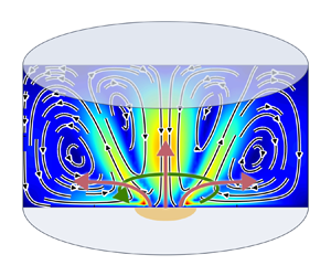
Now, we fix the electric current at $I=1000$ A ($S = 5.3 \times 10^{7}$) and investigate in numerical simulations the EVF under various external magnetic fields. As a reference case, we simulate the EVF without the external magnetic field. The corresponding poloidal and azimuthal velocity fields are presented in figure 9(a,d). The poloidal flow exhibits one fluctuating vortex; similar vortex was shown above for the low electric current. No stable mean azimuthal flow exists in the absence of a vertical magnetic field. The instant distribution of $v_y$ indicates some azimuthal fluctuations.

Figure 9. Instant fields of the poloidal (a–c) and azimuthal (d–f) velocities in the $xOz$ plane in the absence of an external magnetic field (a,d), in the magnetic field ${B_{ext}} = 0.05$ mT (b,e) and in a strong vertical magnetic field ${B_{ext}} = 1$ mT (c, f).

Next, we simulate the flow in the Earth's magnetic field, namely, in the field measured near the laboratory experimental set-up, $B_z=0.05$ mT, $B_x=0.015$ mT. Note that these values differ from those previously described in § 2. This is due to the fact that the magnetic field value used in numerical simulations was measured in the absence of the laboratory set-up. For the experiments, the magnetic field was measured in the same spot, but inside the cell filled with liquid gallium alloy (in the switched-off set-up). The simulations showed that this weak magnetic field is sufficient to essentially suppress the poloidal motion (see figure 9b,e). The remains of the poloidal motion are concentrated in the vicinity of the electrode edges. The azimuthal velocity field shows a developed swirl. Note that the rotation is highly inhomogeneous – the strongest rotation is located in a narrow ring domain, which coincides with the domain of a more intense poloidal flow.

In the strong vertical magnetic field ${B_{ext}} = 1$ mT, the rotational flow penetrates the entire height of the cell, and the azimuthal velocity becomes practically uniform along the height, with the exception of a thin boundary layer near the solid walls (see figure 9a,d). The poloidal flow is manifested by only two pairs of small-scale vortices observed near the upper and lower ends of the cylinder and occurred due to Ekman pumping in viscous layers. Note that the velocity field is symmetric with respect to the vertical field (transferring the electrode to the upper surface will not change the picture).

For a quantitative comparison of the intensities of the poloidal and rotational motions of the metal, we calculate the energy of each flow

(5.1a,b)\begin{equation} {E_{pol}} = \int_V (v^{2}_r + v^{2}_z) \,\mathrm{d}V,\quad {E_{az}} = \int_V v_\varphi^{2} \,\mathrm{d}V, \end{equation}

where $v_r$ and $v_\varphi$ are the radial and azimuthal velocity components. Then, the total energy is ${E_{tot}} = {E_{pol}} + {E_{az}}$. The dependence of these energies on the external magnetic field (see figure 10) shows that the critical value of the field is a value that is sufficient to swirl the metal in such a way that the rotational motion energy becomes comparable to the poloidal EVF energy. This fact was first established by Davidson et al. (Reference Davidson, Kinner, Lingwood, Short and He1999) and illustrated with an EVF in a hemispherical cell with an electrode on the upper free surface. For a cylindrical cell with a bottom electrode, this result has been recently confirmed by Kolesnichenko et al. (Reference Kolesnichenko, Frick, Eltishchev, Mandrykin and Stefani2020). Figure 10 shows that the weak magnetic field (${B_{ext}} \leq 0.01$ mT) does not affect the poloidal motion. At this ${B_{ext}}$, the finite azimuthal energy ${E_{az}}$ is provided by small-scale velocity fluctuations. The global rotational flow develops monotonically with increasing ${B_{ext}}$ as demonstrated in figure 11, where the mean azimuthal velocity at the cell periphery (namely, at $r=0.9R$) is plotted against the applied magnetic field.

Figure 10. Poloidal and azimuthal energies as a function of the external vertical magnetic field. $I=1000$ A. Numerical simulations. An extended version of figure 9 from Kolesnichenko et al. (Reference Kolesnichenko, Frick, Eltishchev, Mandrykin and Stefani2020).

Figure 11. Mean azimuthal velocity at $r=0.9R$ versus the external magnetic field. Here $I=1000$ A.

At ${B_{ext}} \approx 0.01$ mT, the poloidal energy ${E_{pol}}$ starts to decrease and, after the point at which ${E_{pol}} \approx {E_{az}}$, it falls down by two orders of magnitude. Upon reaching the magnetic field ${B_{ext}} \approx 0.04$ mT, both energies ${E_{pol}}$ and ${E_{az}}$ increase, which causes an increase in the magnetic field, and follow a similar power law dependence (close to the linear one), and the poloidal flow energy remains approximately two orders of magnitude less than the azimuthal flow energy. Note that this sharp decrease in the flow energy is accompanied by an equally strong decrease in the level of fluctuations of the flow energy (see figure 12).

Figure 12. Standard deviation (SD) of the poloidal and azimuthal energies versus the external vertical magnetic field. Here $I=1000$ A.

The $E(B)$ dependencies shown in figure 10 cannot be verified experimentally because only the vertical velocity $v_z$ is available for measurement along a few fixed lines (UDV beams). Therefore, we plot the dependence of the Reynolds number $Re$, which characterizes the poloidal motion defined as above through the maximal mean vertical velocity averaged over eight beams, on the external vertical magnetic field. Figure 13 presents the experimental points for the free and solid upper boundary, as well as the results of simulations performed in the same way. The latter (red points in figure 13) confirm that the Reynolds number defined in a localized periphery domain correctly reproduces the dependence ${E_{pol}}({B_{ext}})$ presented in figure 10. The experimental points follow a similar behaviour, but the strong poloidal motion suppression occurs at a stronger external magnetic field, namely, the decrease starts at ${B_{ext}} \approx 0.1$ mT versus ${B_{ext}} \approx 0.02$ mT observed in the numerical simulations. This shift cannot be explained by the presence of the Earth's magnetic field in experiments, because it should provide a shift of the experimental points in the opposite direction. However, the set-up is powered by strong currents and the magnetic fields of the power supply cables can induce fields that are substantially larger than the Earth's field. The current is distributed to the model through a few coaxial cables (see figure 2), but at a distance of approximately $0.7$ m below the cell bottom the cables diverge in opposite directions. Additional numerical studies have shown that the EVF is sensitive to the magnetic field distortion, which can be induced, say, by the power supply cables. Note that the Reynolds numbers calculated in the experiments and simulations are close at a pure EVF (weak magnetic field) and similar at a suppressed state (minimal $Re$), while at a strong field ($1$ mT and more) the experiments demonstrate a stronger intensity of the poloidal motion. The influence of the horizontal component of the magnetic field was studied as well (see the Appendix).

Figure 13. Reynolds number defined through the maximal vertical velocity along the UDV beam vs the applied vertical magnetic field. Results of numerical simulations (red) and experiments with solid (green) and free (blue) upper boundary. Here $I=1000$ A.

6. Dynamics and mechanism of EVF suppression under a vertical magnetic field

We have seen above that the EVF is strongly affected by the magnetic field and demonstrates dramatic changes in the flow pattern even under a weak vertical magnetic field. This flow reorganization is provided by the general metal rotation driven by the Lorentz force produced by the radial component of electric current and applied vertical magnetic field. The general suppression of poloidal motion, as shown by Davidson et al. (Reference Davidson, Kinner, Lingwood, Short and He1999), is due to the typical rotating flows redistribution of the pressure field (Ekman pumping). However, linear combinations of the original EVF and Ekman flows do not yield the structures observed in laboratory and numerical experiments.

For illustration, we show in figure 14 a simple scheme of the vertical velocity profiles along the UDV beam for the pure EVF (curve a) and for the EVF in a vertical magnetic field (curve d). This plot also presents two profiles expected for the flow induced in the cell by a homogeneous radial current in a vertical magnetic field if the surface is free (curve b) or solid (curve c). In both later cases, the poloidal flow is produced by Ekman pumping – note that in the cell with a free surface the flow pattern should be similar to the EVF pattern, and the solid cover causes a two-vortex flow structure to occur. To explain the origin of these profiles, we provide in the same figure schematics of corresponding poloidal flows in the cylindrical cell. It is also worth noting that the EVF under the applied magnetic field (curve d) practically does not depend on the upper boundary, and no direct combination of the EVF and Ekman flows can yield such curves (see figure 7).

Figure 14. Schematic of four kinds of poloidal flow in the cylindrical cell: a pure EVF (a); flows induced by the homogeneous radial current in a vertical magnetic field in the cell with a free surface (b) and with a solid cover (c); a flow associated with the velocity profile, observed in the EVF under a moderate vertical magnetic field (d). Corresponding sketches of vertical velocity profiles along the UDV beam (which is indicated by dashed magenta lines) are shown in the left-hand subpanel.

To understand the flow formation mechanism under the combined action of the poloidal and azimuthal forces, it is essential to analyse the time evolution of the flow pattern after the electric current is turned on. The point is that the evolution of the metal rotation in a relatively weak external magnetic field is a slow process in comparison with the evolution of the EVF itself. Therefore, if the current is switched on at $t=0$, the poloidal flow develops first and dominates until the azimuthal rotation becomes strong enough. Figure 15 illustrates the evolution of the energy of both poloidal and azimuthal flows for approximately 1000 s after the electric current $I=1000$ A was switched on. Two cases are considered: the weak vertical magnetic field (${B_{ext}} = 0.01$ mT), which decreases the poloidal EVF, but is not sufficient to suppress it; and the moderate field (${B_{ext}} = 0.1$ mT), at which the poloidal flow reaches the minimal level of energy at saturated state.

Figure 15. Evolution of the energy of poloidal and azimuthal flows under weak (${B_{ext}} = 0.01$ mT, panel a) and moderate (${B_{ext}} = 0.1$ mT, panel b) magnetic fields after the electric current $I=1000$ A is switched on.

At the very beginning of the process (the graphs start at time $t=0.1$ s), the poloidal energy is two to three orders of magnitude greater than the azimuthal energy and grows like ${\sim } t^{3/2}$ during the first second. Later the poloidal energy growth slows down and the azimuthal energy gradually increases, slower in a weak field, faster and more steadily in a moderate field, but interestingly, in both cases it approaches the poloidal flow energy (approximately $10^{-3}$ (m s$^{-1}$)$^{-2}$) in roughly the same time, $t \sim 40$–$50$ s. After this point, the flows evolve according to very different scenarios. The field ${B_{ext}} = 0.01$ mT is not sufficient to suppress the EVF and an oscillatory mode occurs – both energies oscillate remaining in relation ${E_{pol}}/{E_{az}} \sim 10$. The field ${B_{ext}} = 0.1$ mT completely suppresses the initial EVF, whose energy drops by almost three orders of magnitude. The azimuthal energy continues to rise and the system reaches a state in which ${E_{az}} \sim 500{E_{pol}}$.

We note that if the flow evolves in a spin-up mode, i.e. spinning the metal under a moderate magnetic field after the fast formation of the EVF, the system qualitatively passes through all modes arising for the given current at varying external field. Therefore, we will reproduce step by step such a spin-up mode; but we do this for a lower current, namely $I=100$ A, because it provides more monotonic flow evolution and more stable flow structure.

The poloidal and azimuthal energy at a saturated state versus the external magnetic field for $I=100$ A is shown in figure 16. This figure should be compared with figure 10, in which same graphs are drawn for $I=1000$ A. Both figures are similar. They show that the weaker EVF is suppressed by the lower external field ($5\times 10^{-6}$ T at $I=100$ A versus $4 \times 10^{-5}$ T at $I=1000$ A). The only significant difference concerns the behaviour of azimuthal energy at ${B_{ext}} \to 0$. At $I=100$ A, the azimuthal flow monotonically decreases as the field decreases, while at $I=1000$ A the azimuthal energy does not decrease further at ${B_{ext}} < 2 \times 10^{-5}$ T. As mentioned above, this is due to the fact that at strong currents the EVF flow is unstable and the final level of azimuthal energy in the absence of swirl is due to velocity fluctuations.

Figure 16. Flow energy as a function of the external magnetic field, $I = 100$ A.

Figure 17 illustrates the time evolution of the flow energy at $I=100$A for four different external magnetic fields: ${B_{ext}}=0$ mT (pure EVF); ${B_{ext}}=0.003$ mT (corresponding to the saturated state with ${E_{pol}} \approx {E_{az}}$); ${B_{ext}} = 0.1$ mT; and ${B_{ext}} = 1$ mT. Figure 17(a) shows that without magnetic field the EVF energy starts to increase as $E(t)\sim t^{3/2}$ and follows this law for approximately $10$ s. The growth slows down thereafter, reaching the saturation at $t\approx 300$ s. Note, that there is no regular rotation in a pure EVF and the energy of azimuthal flow in figure 17(a) is due to small-scale fluctuations. During the first second ${E_{az}}\sim t^{3/2}$ following the growth of the poloidal energy, but then lags behind remaining at a very weak level.

Figure 17. Evolution of the energy of poloidal and azimuthal flows without an external magnetic field (pure EVF, panel a), ${B_{ext}} = 0.003$ mT (b), ${B_{ext}} = 0.1$ mT (c) and ${B_{ext}} = 1$ mT (d) after the electric current $I=100$ A is switched on.

At ${B_{ext}} = 0.003$ mT (figure 17b), after a long slow acceleration (approximately 3000 s), the azimuthal flow accumulates the energy comparable with the poloidal flow energy, and this quasi-equilibrium keeps at a saturated state.

Under the external vertical magnetic field ${B_{ext}} = 0.1$ mT (figure 17c), the EVF develops during the first few seconds in the same way as without the field (although its energy is approximately half as weak), but the global rotation grows much faster. Here ${E_{az}}\sim t^{2}$ (the angular velocity grows linearly with time) and ${E_{az}}$ catches up ${E_{pol}}$ at $t\approx 10$ s. After that, the poloidal flow energy decreases, and then the transient process is saturated at ${E_{pol}}\sim 0.003 {E_{az}}$.

Figure 17(d) depicts the evolution of energy under the influence of the strong magnetic field in which the azimuthal flow develops faster than the poloidal one. The poloidal energy increases following the azimuthal energy, but it does not reach it and drops after approximately 30 s, approaching approximately the same level ${E_{pol}}\sim 0.003 {E_{az}}$.

Note that, at saturated states, the flow energy can be stable or can exhibit periodic or chaotic fluctuations. To illustrate this statement, the wavelet spectrograms of normalized poloidal energy fluctuations in a saturated state are shown in figure 18 for three cases. The first corresponds to the mode from figure 15(a), in which the poloidal motion dominates. The second concerns the opposite case (a strong swirl and a very weak poloidal flow), shown in figure 15(b). Both spectrograms demonstrate stochastic fluctuations in the range of characteristic frequencies. The third spectrogram shows very strong regular fluctuations that occur at a lower current and a stronger magnetic field ($I=100$ A, ${B_{ext}} = 1$ mT); the energy evolution is shown in figure 17(d).

Figure 18. Wavelet spectrograms of the poloidal energy fluctuations at saturated state. Here (a) $I = 1000$ A, ${B_{ext}} = 0.01$ mT, (b) $I = 1000$ A, ${B_{ext}} = 0.1$ mT, (c) $I = 100$ A, ${B_{ext}} = 1$ mT.

Figure 19 shows how the flow pattern changes during this evolution for the case ${B_{ext}}=0.1$ mT, $I=100$ A considered in figure 17(c). At the beginning of the evolution (figure 19a–c) the poloidal EVF is similar to a pure EVF, and the rotating flow is concentrated near the electrode. The maximal angular velocity is quite high (figure 19c, f,i,l,o,r), but the total angular momentum is weak. Thus, the inhomogeneous current distribution provides strong axial and radial differential rotations.

Figure 19. Evolution of the EVF flow at $I=100$ A and ${B_{ext}} = 0.1$ mT. The poloidal (a,d,g,j,m,p) and azimuthal (b,e,h,k,n,q) velocity fields in the $x0z$ plane, and the angular velocity along the cell axis (c, f,i,l,o,r) for six time moments, $t=6.2$, $60$, $92$, $122.1$, $160.6$ and $478.6$ s.

Figure 19(c, f,i,l,o,r) shows the distribution of the flow angular velocity $\omega$ along the cell axis. The developing azimuthal flow with a strong decrease of the angular velocity with height leads to the formation of a domain with reduced pressure above the electrode. The vertical pressure drop causes a downward flow to occur along the cell axis. This downward flow results in a second large-scale poloidal cone-shaped vortex in the upper central part of the cell (figure 19d–f). The azimuthal flow is still concentrated close to the electrode, but it is stretched along the cone.

The downward poloidal vortex is formed at $t \approx 100$ s, being accompanied by a sharp decrease in the poloidal flow energy. The increase of the swirl leads to further suppression of the poloidal flow (figure 19g–i). The upper toroidal vortex begins to dominate in the cell, and the azimuthal flow spreads up to the upper boundary.

Figure 19(j–l) corresponds to the minimal energy of the poloidal flow (the strongest suppression). The upper vortex continues to grow and the azimuthal flow occupies practically the whole cell. As the swirl is increased further, the one-vortex flow develops. Only a weak residual toroidal vortex survives at the periphery of the bottom, which is the result of Ekman pumping (figure 19m–o). At fast rotation, this poloidal flow becomes unstable (figure 19p–r) , while the azimuthal flow demonstrates a solid-like rotation. The angular velocity is constant along the most part of the cell axis, keeping a maximum near the electrode. This domain of the highest swirl provides the stable axial downward flow.

Figure 20 illustrates the flow pattern evolution in the presence of a strong magnetic field (${B_{ext}} = 1$ mT), in which the azimuthal flow develops first (the case shown in figure 17d). Then the intense azimuthal swirl appears as a localized vortex in the vicinity of the electrode, providing a downward axial flow (figure 20a–c). The swirl spreads rapidly through the cell and at $t\approx 25$ s it occupies the entire domain. It is at this moment that the poloidal motion begins to decrease and saturate. The final state is similar to that observed in the previous case (compare figures 19p–r and 20g–i).

Figure 20. Evolution of the EVF flow at $I=100$ A and ${B_{ext}} = 1$ mT. The poloidal (a,d,g) and azimuthal (b,e,h) velocity fields in the $x0z$ plane, and the angular velocity along the cell axis (c, f,i) for three time moments $t = 5$, $25$ and $300$ s.