2.1 AIS data preprocessing

Detection of scenes of near miss is based on an extensive analysis of information obtained from AIS data. The AIS transmits certain information about the navigational status of the ship to other ships in the vicinity and shore-based stations, continuously and automatically (Tixerant et al., Reference Theodoropoulos, Tritsarolis and Theodoridis2018). The application of AIS is meaningful in protecting the marine environment, ensuring the safety of life at sea, improving the safety of navigation, and developing the shipping industry efficiently. The types of AIS data used by this paper are summarised in Table 1.

Table 1. Types of AIS data used in this paper

The updating speed of AIS data varies with the ship's navigation status, so information on the ship's trajectory may not be received at the same time. The rate of data transmission is seen in Table 2. In the process of AIS data transmission, due to the limitations of equipment, weather, sea conditions and other factors, information is often missing, so a ship's trajectory obtained from AIS data is a discrete space-time sequence. Time synchronisation interpolation is needed to obtain time synchronous and continuous ship trajectory data because it is necessary to have a fixed sampling frequency for detecting the scenes of near miss. The process of time synchronisation interpolation is shown in Figure 1. The blue points represent the original trajectory data of ship A, the yellow points represent the original trajectory data of ship B, the red points represent the new trajectory data of ship A, and the green points represent the new trajectory data of ship B. It can be seen that the original trajectory data of ship A and ship B are not synchronised in time and the interval is not equal. After synchronous interpolation, the trajectory data with fixed sampling frequency is obtained, where t ₁ to t ₈ are interpolation time points. The original trajectory points of ship A at t ₃ and t ₈ and the original trajectory points of ship B at t ₁ and t ₄ should not be interpolated, because they are all at the interpolation time points. The interpolation calculation of ship position data is as follows:

(1)\begin{align}\lambda & = {\lambda _1} + \frac{{{\lambda _2} - {\lambda _1}}}{{{t_2} - {t_1}}}t - {t_1}\end{align}

(2)\begin{align}\varphi & = {\varphi _1} + \frac{{{\varphi _2} - {\varphi _1}}}{{{t_2} - {t_1}}}t - {t_1}\end{align}

where ${\lambda _1}$ is the longitude at t ₁; $\textrm{\; }{\varphi _1}$ is the latitude at t ₁; ${\lambda _2}$ is the longitude at t ₂; ${\varphi _2}$ is the latitude at t ₁; $\varphi$ is the latitude at t; $\lambda$ is the longitude at t.

Figure 1. Synchronous interpolation process

Table 2. Sample rate of variable data from AIS (Norris, Reference Lewisson2007)

To ensure the correctness of the interpolation, it is also necessary to segment the ship's trajectory. If the time interval between two adjacent points in a ship's trajectory data is too large, the track should be segmented between the two points. If the amount of sub-trajectory data after segmentation is too small, it should be deleted because it cannot provide important information (Theodoropoulos et al., Reference Szlapczynski and Szlapczynska2020).

2.2 Model for detecting the scenes of near miss based on arena

Scholars have considered using DCPA and TCPA to detect the scenes of near miss, but these do not fully reflect the severity level of encounters (Zhang et al., Reference Zhang and Meng2015). The distance between the two ships is also an important factor to detect scenes of near miss, but there are no conclusions about the relationship between the scene of near miss and the distance between the two ships. Therefore, the relationship between the distance and scene of near miss is further analysed according to the Convention on the International Regulations for Preventing Collisions at Sea (COLREGS). Generally, the process of collision accident between ships can be divided into four stages, shown in Figure 2.

Figure 2. Four stages of a ship collision accident

The first stage is where there is no risk of collision as the ships are a long distance apart. At this stage, because of the long distance, it is considered that there is no collision-related risk at this time. From a quantitative perspective, the distance between the two ships (D₁) should be at least 6 nm. The second stage is when collision danger occurs, i.e., two ships approach each other and meet the requirements of Rule 7, ‘Collision danger’ of COLREGS (IMO, Reference Szlapczynski and Szlapczynska1972). Note that the collision risk is not defined by COLREGS, and there are no corresponding provisions for the applicable distance between two ships in the event of collision danger. However, from the legal minimum visible distance of the semaphore, the distance between the two ships (D₂) at this stage can be between 3 and 6 nm. The third stage is an urgent situation. In terms of maritime practice, it is generally believed that an urgent situation is when two ships approach each other. Safe distance is the distance from the ship's centre to the border of the ship's domain. In the event of an urgent situation, the distance between the two ships (D₃) is at least the distance of the ship domain and the turning distance required for ships to take action to avoid a collision. The fourth stage is an imminent danger situation. Determining the extent to which the distance (D₄) is close is difficult when two ships are in an imminent danger situation. However, maritime researchers consider that an imminent danger situation is where one ship cannot avoid a collision by itself when the other ship is approaching.

A ship's domain is the area around the ship that should be avoided by other ships for safety reasons. Ship domain is a special form of safe distance, because the distance between the ship and its domain boundary differs according to various bearings. Since Fujii introduced the concept of ship domain, researchers have been making statistical analyses of the distances between ships at the scenes of encounters, and calculating the size of the domain according to expert experience (Szlapczynski and Szlapczynska, Reference Sormunen, Hänninen and Kujala2017; Im and Luong, Reference Im and Luong2019; Zhang and Meng, Reference Yoo2019; Fiskin et al., Reference Fiskin, Nasiboglu and Yardimci2020). The concept of ship domain is widely used in maritime research on near miss detection (Wu et al., Reference Wang, Meng, Xu and Wang2016; Zhang et al., Reference Zhang, Goerlandt, Montewka and Kujala2016; van Westrenen and Ellerbroek, Reference Tixerant, Guyader, Gourmelon and Queffelec2017; Pietrzykowski et al., Reference Norris2018; Zhang et al., Reference Zhang, Floris, Pentti and Yinhai2019).

The size of a ship's domain can vary quite significantly (Wang et al., Reference Wang, Meng, Xu and Wang2009), and the application of different domains to detect near miss affects the detection results. The Fujii ship domain is small, and can only be used to detect the most critical encounters (Goerlandt et al., Reference Goerlandt, Montewka, Lammi and Kujala2012). However, few of the most critical encounters occur in open waters, which makes this method of analysing marine traffic risks inefficient. Therefore, it should be noted that lower potential risk encounters in open waters are also worthy of attention. All the scenes of encounter with potential risk are defined as scenes of near miss in this paper.

In terms of maritime practice, the officer responsible should take appropriate collision avoidance actions to clear other ships. When the officer starts collision avoidance manoeuvres to avoid other ships, it can be assumed that the officer realises the potential risk of collision. Based on the above situation, as a criterion for detecting the scenes of potential risk encounters, this study proposes using the distance between two ships when a ship starts to turn because of the threat from the other ship. To calculate this distance, the expert questionnaire method was adopted in the process of data collection (Davis et al., Reference Davis, Dove and Stockel1980). On the basis of statistical data analysis, a ship domain named an ‘arena’ is obtained, which consists of an off-centre circle.

Both the arena and Fujii ship domain of a ship are shown in Figure 3. The centre of the arena circle is an assumed ship position; the orientation of the real ship is 199° to the assumed ship and a distance of 1⋅7 nm away. The real ship will be involved in a near miss if the other ship sails into the arena. Target ship 1 is within the arena, which means that a near miss occurs between target ship 1 and the real ship. Target ship 2 is not in the arena, which means that no near miss occurs between target ship 2 and the real ship.

Figure 3. Arena and Fujii ship domain

Note that, in a scene of encounter, one ship is usually taken as the research object, which is defined as ‘own ship’, to analyse the relationship between it and other ships. In the model for detecting a near miss, real ship is setected as research object, so ‘own ship’ represents real ship. The model for detecting a near miss is described using Equations (3)–(6), where $\varphi$ is the heading of own ship; $Lo{n_{\textrm{real}}}$ is the longitude of real own ship; $La{t_{\textrm{real}}}$ is the latitude of real own ship;$\; Lo{n_{\textrm{assumed}}}$ is the longitude of assumed own ship; $La{t_{\textrm{assumed}}}$ is the latitude of assumed own ship; $Lo{n_{\textrm{target}}}$ is the longitude of target ship; $La{t_{\textrm{target}}}$ is the latitude of target ship; ${f_{\textrm{Arena}}} \le 0$ represents own ship involved a near miss, and ${f_{\textrm{Arena}}} > 0$ represents own ship not involved in a near miss.

(3)\begin{align}& \begin{cases} {Lo{n_{\textrm{assumed}}} = Lo{n_{\textrm{real}}} + 1{\cdot}7 \times \textrm{sin}({\varphi + {{19}^\circ }} )}\\ {La{t_{\textrm{assumed}}} = La{t_{\textrm{real}}} + 1.7 \times \textrm{cos}({\varphi + {{19}^\circ }} )} \end{cases}\end{align}

(4)\begin{align}& d = \sqrt {{{({Lo{n_{\textrm{assumed}}} - Lo{n_{\textrm{target}}}} )}^2} + La{t_{\textrm{assumed}}} - La{t_{\textrm{target}}}^2} \end{align}

(5)\begin{align}& {f_{\textrm{Arena}}} = d - 2{\cdot}7\end{align}

(6)\begin{align}& \begin{cases} {{f_{\textrm{Arena}}} > 0}& \hbox{while target ship is out of own ship's Arena}\\ f_{\textrm{Arena}} = 0 & \hbox{while target ship is on own ship's Arena}\\ {{f_{\textrm{Arena}}} < 0}& \hbox{while target ship is in own ship's Arena} \end{cases}\end{align}

2.3 Statistical model for near miss based on water grid method

The water grid method is usually used to study macroscopic collision risk based on geographical distribution (Qu et al., Reference Pietrzykowski, Siemianowicz and Wielgosz2011; Kim and Jeong, Reference Kaneko2016; Wu et al., Reference Wang, Meng, Xu and Wang2016). The advantage of the water grid method is that it organically combines the prediction model built by water traffic survey with the future prediction to form a new closed-loop risk assessment method for a port water traffic environment. To some extent, it avoids the superficial evaluation available by qualitative method, and has the characteristics of grid dynamics. According to the influence of different offshore distances on marine traffic, a certain water area is divided into several kinds of grid squares, whose size depends on the geographical location and size of the research object. The typical grid squares are divided into shoreline grid squares, near shore grid squares, far shore grid squares and open sea grid squares, and the squares become larger with the increase of offshore distance. In open waters, it is more convenient to study the collision risk of ships by dividing a certain water area into several grid squares with the same side length. This study divides the research water area into several grid squares having a side length of 2 nm. Because COLREGS stipulate that DCPA should not be <2 nm for the low visibility case (Fang et al., Reference Fang, Yu, Ke, Shaw and Peng2018), this study stipulates the basis for determining the grid size.

A single near miss is defined in this paper, which is the whole progress from target ship sailing into the arena of own ship to leaving it. However, a ship involved in a near miss often crosses multiple grid squares. If the whole process is recorded as a single near miss, it is difficult to determine to which grid square the scene of the near miss belongs. Moreover, the sampling frequency of AIS data affects the results of detection of scene of near miss, and can have a negative impact on marine traffic risk analysis (Goerlandt et al., Reference Goerlandt, Montewka, Lammi and Kujala2012). To solve the above problems, each gird square is regarded as an independent research object, and ship trajectory data with fixed sampling frequency are used to detect whether each ship is continuously involved in the same scene of near miss in this grid square. If it is, it should be recorded as a single near miss; if not, the number of near misses should be calculated according to the ship trajectory data. A ship trajectory in a single grid square is shown in Figure 4: the red point represents the trajectory point where the ship is involved in a near miss, and the green point represents the trajectory point where the ship is not involved in a near miss. It can be seen that the ship is involved in two scenes of near miss, one is between t ₂ and t ₃, the other is t ₅ to t ₇. Therefore, the number of scenes of near miss of this ship in this grid square should be recorded as two.

Figure 4. Ship trajectory in a single grid square

Based on the above, a statistical model for the scenes of near miss based on the water grid method is proposed. As shown in Figure 5, to illustrate the statistical method based on near miss in each grid square of this study, we assume that the red ship is in the centre of grid square #1, and maintains the heading at 45°; the green ship turns to the right; the red ship and the yellow ship are sailing at the same heading and speed during t ₁ to t ₂, whereas the yellow ship turns to the right after t ₂.

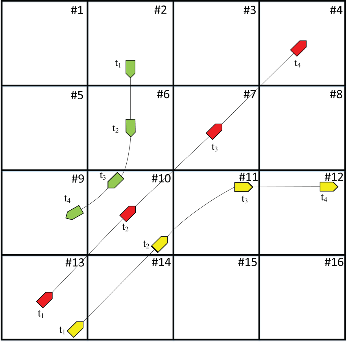
Figure 5. Meeting of red ship, green ship and yellow ship

During the period from t ₁ to t ₄, the green ship sailed through the grid squares #2, #6, #9 and #10; the red ship sailed through the grid squares #4, #7, #10 and #13; and the yellow ship sailed through the grid squares #10, #11, #12, #13 and #14. The numbers of ships sailing through each grid square are shown in Table 3, where M represents the number of ships.

Table 3. Number of ships sailing through each grid square

In encounter scenes, one ship is usually taken as the research object, which is defined as ‘own ship’, to analyse the relationship between it and other ships. For the ships involved in the same encounter, one ship can be selected as own ship, and the other ships are target ships. The scene in Figure 5 can be divided into three different senses according to different own ships: the red ship is selected as own ship, the green ship is selected as down ship, and the yellow ship is selected as own ship. The three senses are shown as Figures 6–8.

Figure 6. The red ship is selected as own ship

Figure 7. The green ship is selected as own ship

Figure 8. The yellow ship is selected as own ship

In Figure 6, the red ship and the yellow ship are sailing at the same heading and speed during t ₁ to t ₂, so the yellow ship remains in the red ship's arena until the yellow ship turns right to leave it after t ₂. In grid square #13, the yellow ship is sailing in the red ship's arena, so the number of scenes of near miss in which the red ship was involved, is one in grid square #13. In grid square #10, both the yellow ship and the green ship are sailing in the red ship's arena, so near misses occur between the yellow and red ships and between the green and red ships, respectively. Therefore, the number of scenes of near miss in which the red ship was involved is two in grid square #10.

In Figure 7, the red ship entered the green ship's arena at t ₂, and then the green ship turned right after t ₂. The red ship left the green ship's arena before the green ship entered grid square #10. Therefore, the number of scenes of near miss in which the green ship involved is only one in grid square #6.

In Figure 8, the red ship and the yellow ship are sailing at the same heading and speed during t ₁ to t ₂, so the red ship remains in the yellow ship's arena until the yellow ship turns right to leave after t ₂ in grid square #10. Therefore, the number of scenes of near miss in which the yellow ship was involved in grid square #10, #13, and #14 was one in all cases.

To sum up, the numbers of scenes of near miss in each grid square are shown in Table 4, where N is the number of near misses. Note that a ship should be considered to be in a certain grid square when the ship's position is on the right or upper boundary of this grid square, and the ship should not be considered to be in a certain grid square when the ship's position is on the left or lower boundary of this grid square. The flow chart of the statistical model for the scenes of near miss based on the water grid method is shown in Figure 9.

Figure 9. The flow chart of statistical model for near miss based on water grid method

Table 4. Number of near misses occurring in each grid square

2.4 Macroscopic collision risk model based on near miss

Compared with the research of microscopic collision risk, the research and application of macroscopic collision risk is still at a very early stage, and the research methods used are mostly focused on statistical analysis. The research on macroscopic collision risk can be divided into the following four categories of macroscopic collision risk based on: collision frequency (Cockroft, Reference Cockroft1981, Reference Cockroft1982), encounter frequency (Goodwin, Reference Goodwin1978; Lewisson, Reference Le, Ding, Dong and Zhang1978; Kaneko, 1972), collision probability (Le et al., Reference Lappalainen, Vepsäläinen, Salmi and Tapaninen2011), or geographical distribution (Qu et al., Reference Pietrzykowski, Siemianowicz and Wielgosz2011; Goerlandt et al., Reference Goerlandt, Montewka, Lammi and Kujala2012; Zhang et al., Reference Zhang and Meng2015, Reference Zhang, Goerlandt, Montewka and Kujala2016; Kim and Jeong, Reference Kaneko2016; Yoo, Reference Wu, Mehta, Zaloom and Craig2018).

Generally, the number of marine traffic accidents and encounters that occur show the risk in certain waters; the larger the number, the higher the risk. However, there are few accidents, so accidents alone cannot fully show the marine traffic risk. On the other hand, long-distance encounters usually mean that there is no potential risk between two ships, so this method cannot accurately evaluate the marine traffic risk. In this study, all the scenes of potential risk encounters are detected, and treated as ‘near miss’.

There is no strong positive correlation between the marine traffic risk and the traffic flow, because waters with large traffic flow and small number of near misses should be considered as low marine traffic risk areas. Therefore, marine traffic risk is associated with traffic flow, the ratio of the number of near misses in the study water to the total number of ships is used as an index to evaluate the marine traffic risk, which represents the average number of near misses of each ship in the study water. The macroscopic collision risk model based on near miss is represented by macroscopic collision risk (MCR) which is concerned with the number of scenes of near miss and traffic flow. MCR is defined as follows:

(7)\begin{equation}\textrm{MCR} = N/M\end{equation}

where N is the number of scenes of near miss; M is the number of ships sailing through the water area.

Assume two groups of data in the same water: one is that the number of scenes of near miss is 10 and the number of ships is 100, and the other is that the number of scenes of near miss is 10 and the number of ships is 1,000. Considering only the number of scenes of near miss, the result of evaluating the marine traffic risk of the two groups should be the same. However, considering the factor of traffic flow, the number of ships in the first group is smaller, so the risk should be greater. Using this model to evaluate the marine traffic risk of the above example, the results are 0⋅1 and 0⋅01 respectively, which are more similar to the real marine traffic risk.