


Introduction
Since the dawn of modern evolutionary synthesis (Huxley Reference Huxley1942), macroevolution in deep time has often been considered as resulting mainly from the effects of extrinsic (environmental) factors such as climate change. In addition, random genetic mutations have been thought to produce isotropic variation upon which natural selection acts as a filter, driving the survivors toward fitness peaks (Mayr Reference Mayr1982; Wright Reference Wright1982; Wainwright Reference Wainwright2007; Condamine et al. Reference Condamine, Rolland and Morlon2013). Yet the question of the relative role of intrinsic (e.g., developmental) factors in macroevolution remains scarcely addressed (Erwin Reference Erwin2017; Jablonski Reference Jablonski2017). Organisms and their shapes are constrained by the universal rules of chemistry, physics, and geometry. The set of theoretically possible forms is thus bounded by the way these forms are generated during ontogeny. In other words, developmental processes determine the variation of individuals anisotropically, thus possibly biasing evolution along favorable paths.
Because organisms and environment “actively co-determine each other” (Levins and Lewontin Reference Levins and Lewontin1985: p. 89), the dichotomy between intrinsic and extrinsic factors is necessarily reductive, and we should expect that explanatory schemes will involve both types of factors. Schluter (Reference Schluter1996) first proposed that the main direction of genetic variance (termed Gmax) within a population corresponds to a “line of least resistance” to evolution, that is, evolution will occur more easily, and thus more frequently, in that direction rather than in any other. Interestingly, as phenotypic and genetic variance–covariance matrices are correlated (Siahsarvie Reference Siahsarvie2012), the main direction of phenotypic variance (Pmax) is aligned with Gmax. The theory of lines of least resistance can thus be extended to the phenotypic variance of a population, extant or fossil (in which case, we prefer the term “assemblage”). Moreover, phenotypes do not contain information only about the development of the individuals, but also about their environment. Hence, this theoretical framework can be used to assess the relative roles of environmental and developmental processes in evolution via the analysis of the main directions of phenotypic variance in fossil assemblages (Renaud et al. Reference Renaud, Auffray and Michaux2006; Hunt Reference Hunt2007). The Pmax can be interpreted in terms of genetic/developmental constraints, and any significant deviation from Pmax can be interpreted as being the consequence of an environmental disturbance. To conduct such studies in deep time, one needs a framework with a fossil record that spans a large time frame and comprises large assemblages that are available at a temporal resolution that compares with the dynamics of paleoenvironmental fluctuations. Conodonts fit these requirements.
Conodonts are a group of extinct, jawless marine organisms that are considered vertebrates (Donoghue et al. Reference Donoghue, Forey and Aldridge2000). They are mainly known in the fossil record by their tiny, apatitic teeth-like feeding elements. Their feeding apparatus usually includes 15 elements. The anteriorly located group of so-called S and M elements was likely used to grasp food (Goudemand et al. Reference Goudemand, Orchard, Urdy, Bucher and Tafforeau2011), and in the posterior part of the mouth, two pairs of so-called P elements were used to process the food (Purnell Reference Purnell1994; Martínez-Pérez et al. Reference Martínez-Pérez, Purnell, Rayfield and Donoghue2016). Throughout their 300 Myr of existence (from the late Cambrian to the Late Triassic), conodonts have one of the best spatiotemporally resolved fossil record and are often used as index fossils for relative dating of sediments and stratigraphic correlation between geological sites. Because conodont elements are also used for geochemistry-based reconstructions of paleoenvironments (Wenzel et al. Reference Wenzel, Lécuyer and Joachimski2000; Joachimski et al. Reference Joachimski, Pancost, Freeman, Ostertag-Henning and Buggisch2002, Reference Joachimski, von Bitter and Buggisch2006; Trotter et al. Reference Trotter, Williams, Barnes, Lécuyer and Nicoll2008; Sun et al. Reference Sun, Joachimski, Wignall, Yan, Chen, Jiang, Wang and Lai2012), they are an ideal model system for deep-time evolutionary studies. However, until recently, conodonts were used almost exclusively in an “utilitarian” way (for biostratigraphy and paleoenvironmental reconstructions), and despite their huge potential, they have remained relatively underexploited for evolutionary studies, and virtually nothing is known about functional or developmental constraints in conodonts (Purnell Reference Purnell1994; Donoghue and Purnell Reference Donoghue and Purnell1999; Girard et al. Reference Girard, Renaud and Sérayet2004b; Girard and Renaud Reference Girard and Renaud2007; Goudemand et al. Reference Goudemand, Orchard, Urdy, Bucher and Tafforeau2011; Murdock et al. Reference Murdock, Sansom and Donoghue2013; Martínez-Pérez et al. Reference Martínez-Pérez, Plasencia, Jones, Kolar-Jurkovšek, Sha, Botella and Donoghue2014a, Reference Martínez-Pérez, Rayfield, Purnell and Donoghueb, Reference Martínez-Pérez, Purnell, Rayfield and Donoghue2016). Qualitative descriptions of conodont element variation are ubiquitous in the literature, as they are standard in conodont systematics. Yet these descriptions are usually restricted to given species, they rarely focus on patterns of covariation, and the lack of quantification implies that they cannot be statistically evaluated.
Quantitative studies on conodont elements are made difficult by their lifelong accretionary mode of growth (Donoghue Reference Donoghue1998): growth lamellae are periodically added around the elements, resulting in an increase of the number of denticles and a modification of the length:height ratio of the element during ontogeny, thereby hindering definition and identification of homologous landmarks and complicating biologically relevant comparisons (Jones et al. Reference Jones, Purnell and von Bitter2009). Previous quantitative analyses on conodont elements were based on classical and/or geometric morphometrics and quantified interspecific (Croll et al. Reference Croll, Aldridge and Harvey1982; Murphy and Cebecioglu Reference Murphy and Cebecioglu1984; Klapper and Foster Reference Klapper and Foster1993; Girard et al. Reference Girard, Renaud and Korn2004a; Chen et al. Reference Chen, Beatty, Henderson and Rowe2009; Girard and Renaud Reference Girard and Renaud2011) or intraspecific variation (Murphy and Springer Reference Murphy and Springer1989; Ritter Reference Ritter1989; Jones et al. Reference Jones, Purnell and von Bitter2009; Chen et al. Reference Chen, Neubauer, Krystyn and Richoz2016). Some authors further described evolutionary trends (Barnett Reference Barnett1972; Roghi et al. Reference Roghi, Mirro and Vecchia1995; Girard and Renaud Reference Girard and Renaud2007; Jones Reference Jones2009) or linked some morphological evolutions to paleoenvironmental changes (Barnett Reference Barnett1972; Renaud and Girard Reference Renaud and Girard1999; Girard et al. Reference Girard, Renaud and Sérayet2004b; Girard and Renaud Reference Girard and Renaud2008), paleobiogeography (Tolmacheva and Löfgren Reference Tolmacheva and Löfgren2000), or functional aspects (Purnell Reference Purnell1994; Martínez-Pérez et al. Reference Martínez-Pérez, Plasencia, Jones, Kolar-Jurkovšek, Sha, Botella and Donoghue2014a, Reference Martínez-Pérez, Rayfield, Purnell and Donoghueb, Reference Martínez-Pérez, Purnell, Rayfield and Donoghue2016). For instance, Croll and coworkers (Reference Croll, Aldridge and Harvey1982) used biometry (length of different parts of the element, angle measurements for denticle inclination, and curvature of the element) to describe the P1 elements of Ozarkodina, Pryantodina, Carniodus, Microzarkodina, and Pterospathodus and concluded that biometry could be used for classification and identification. Renaud and Girard (Reference Renaud and Girard1999) studied the response of Icriodus and Palmatolepis to Late Devonian extreme paleoenvironmental perturbations in terms of the P1 element's oral outline, showing that the response of the two genera differed in time, which the authors interpreted as different sensitivities to the environmental disturbance and, hence, possibly different habitat preferences. Jones (Reference Jones2009) used biometry and outline analyses on Silurian material of Pterospathodus to test for morphological temporal trends and observed that they involved mainly allometric repatterning. Yet, so far, no study has focused on patterns of covariation between different traits of a given element to investigate developmental constraints and putative evolutionary paths of least resistance within the conodont morphospace.
Here we study the morphological variation around the Carnian/Norian boundary (CNB, Late Triassic, ca. 227 Ma) of P1 elements from the Pizzo Mondello section (Sicily, Italy) (Mazza et al. Reference Mazza, Rigo and Gullo2012b) with geometric morphometrics. These conodont elements belong to four genera and seven species: Carnepigondolella pseudodiebeli and Carnepigondolella zoae; Hayashiella tuvalica; Epigondolella quadrata, Epigondolella rigoi, and Epigondolella uniformis; and Metapolygnathus communisti. The material corresponds to a time interval that directly follows the Carnian pluvial episode (Julian/Tuvalian boundary crisis, 234–230 Ma), which was marked not only by a conodont extinction (Rigo et al. Reference Rigo, Preto, Roghi, Tateo and Mietto2007), but also by major floral and faunal turnovers (Simms and Ruffell Reference Simms and Ruffell1990; Hallam Reference Hallam and Walliser1996; Roghi et al. Reference Roghi, Gianolla, Minarelli, Pilati and Preto2010). The corresponding species illustrate one of the last documented conodont evolutionary radiations before their final demise at the Triassic/Jurassic boundary (201.3 Ma) (Pálfy et al. Reference Pálfy, Demény, Haas, Carter, Görög, Halász, Oravecz-Scheffer, Hetényi, Márton and Orchard2007; Mazza et al. Reference Mazza, Rigo and Gullo2012b; Mazza and Martínez-Pérez Reference Mazza and Martínez-Pérez2015). This material was selected because of its excellent preservation, the relative abundance of elements in each sample/species, and the fact that it has been already the subject of extensive sampling (this section is a candidate for the GSSP of the base of the Norian [Nicora et al. Reference Nicora, Balini, Bellanca, Bertinelli, Bowring, Di Stefano and Dumitrica2007]) and several in-depth analyses, including a cladistic analysis (Mazza et al. Reference Mazza, Cau and Rigo2012a), paleoenvironmental reconstructions (Muttoni et al. Reference Muttoni, Kent, Olsen, Di Stefano, Lowrie, Bernasconi and Hernández2004; Mazza et al. Reference Mazza, Furin, Spötl and Rigo2010), and several ontogenetic series reconstructions in particular using synchrotron imaging (Mazza and Martínez-Pérez Reference Mazza and Martínez-Pérez2015). Ancestor–descendant relationships were also hypothesized between most of the species present in the Pizzo Mondello section. Concerning the studied data set (five genera), two lineages can be recognized, with the genus Paragondolella as their presumed common ancestor. Note that alternative systematics and associated phylogenetic and ancestor–descendant relationship hypotheses have been proposed for a similar conodont assemblage from Black Bear Ridge, British Columbia, Canada (Orchard Reference Orchard2013, Reference Orchard2014). Yet these hypotheses are based on a phenetic analysis and have not been tested quantitatively.
Mosher (Reference Mosher1968) and, later, Mazza and coworkers (Reference Mazza, Rigo and Gullo2012b) have already proposed hypotheses of putative evolutionary trends based on these taxa during the CNB interval. They suggested the derivation of Metapolygnathus and Epigondolella from the polyphyletic genus Carnepigondolella, through a series of newly derived characters: (1) the shifting of the pit, (2) the shortening of the platform, (3) the shortening of the anterior trough margin, (4) modifications of the lower margin profile of the platform, (5) the appearance of a stronger platform ornamentation (evolution of Carnepigondolella into Epigondolella), and (6) modifications of the size and relative location of the cusp. Trends 1, 2, 3, and 5 have also been described in Black Bear Ridge (Orchard Reference Orchard2014) for the lineages crossing the CNB (see Rigo et al. [2018] for a discussion).
In this work, we analyze the quantitative morphological variation of P1 conodont elements within and between these seven morphospecies and their evolution within 7 Myr around the CNB. We focus on the exploration of this data set for recurrent patterns, especially patterns of variation and covariation between traits.
Materials and Methods
The samples are housed in the collections of the Dipartimento di Scienze della Terra “A. Desio” (Università degli Studi di Milano). All samples are from the Pizzo Mondello section in the Sicani Mountains, western Sicily, Italy (Mazza et al. Reference Mazza, Rigo and Gullo2012b); they are dated between the latest Carnian and the earliest Norian. Conodonts from this section have an average color alteration index (CAI) of 1–1.5, indicating minimal postdepositional heating (Epstein et al. Reference Epstein, Epstein and Harris1977; Nicora et al. Reference Nicora, Balini, Bellanca, Bertinelli, Bowring, Di Stefano and Dumitrica2007). The specimens were selected to be as complete as possible. A set of 8 to 24 P1 elements per species were 3D scanned, a total of 132 P1 elements were considered (Table 1). According to the time calibration (Kent et al. Reference Kent, Olsen and Muttoni2017: Fig. 7), the assemblage spreads over 7 Myr (230.5–222 Ma).
Table 1. List of the studied material: specific determination, age, stratigraphic location (sample number), number of specimens, and ontogenetic stage (sensu Mazza and Martínez-Pérez Reference Mazza and Martínez-Pérez2015). As H. tuvalica was not included in that study, the corresponding ontogenetic stages were determined after the illustrations of Mazza et al. (Reference Mazza, Cau and Rigo2012a: Plate 3, Figs. 3–10).
Based on the cladistic analysis by Mazza et al. (Reference Mazza, Cau and Rigo2012a) (Fig. 1), the five genera considered here are closely related. In particular, Metapolygnathus is closest to C. zoae, whereas Epigondolella is closest to C. pseudodiebeli. The affinity of Hayashiella remains unclear. These authors also hypothesized that both Metapolygnathus and Epigondolella would derive from the paraphyletic genus Carnepigondolella. Note that Epigondolella is considered as polyphyletic since the discovery of evolutionary convergences within this genus (Mazza and Martínez-Pérez Reference Mazza and Martínez-Pérez2016). Furthermore, more recent studies on the phylogeny and evolution of the metapolygnathids (Mazza et al. Reference Mazza, Nicora and Rigo2018) led to the hypothesis that the lineage Metapolygnathus praecommunisti–Metapolygnathus dylani–Metapolygnathus parvus is probably phylogenetically closer to the paragondolellids than it is to the carnepigondolellids; whereas the more ornate metapolygnathids (i.e., Metapolygnathus mersinensis and Metapolygnathus mazzai) would be more closely related to Carnepigondolella. This new interpretation, however, is compatible with the results provided by the previous cladistic analysis. The phylogenetic revision of Epigondolella does not affect its relationship with Carnepigondolella. Paragondolella polygnathiformis and Paragondolella praelindae were the last two conodont species of Paragondolella to survive the Julian/Tuvalian boundary crisis caused by the Carnian pluvial episode. This genus is considered as the last common ancestor of Norigondolella, Carnepigondolella, Epigondolella, and Metapolygnathus. More precisely, P. praelindae is considered the ancestor of the genus Norigondolella, whereas Paragondolella noah is the ancestor of the genus Carnepigondolella (Mazza et al. Reference Mazza, Cau and Rigo2012a).
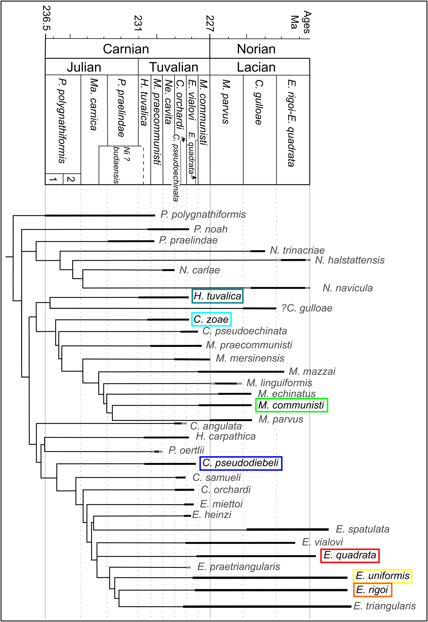
Figure 1. Simplified, stratigraphically calibrated, global strict consensus tree topology (modified after Mazza et al. [2012b] for the cladogram, after Rigo et al. [2018] for the species ranges and the biozonation); C., Carnepigondolella; E., Epigondolella; H., Hayashiella; Ma., Mazzaella; M., Metapolygnathus; Ne., Neogondolella; Ni.?, Nicorraella?; P., Paragondolella. The taxonomy has been modified according to recent updates (after 2012), and the range of species absent (Rigo et al. Reference Rigo, Mazza, Karádi, Nicora and Tanner2018) are represented by dashed lines. Hayashiella tuvalica includes the Tuvalian forms of Carnepigondolella nodosa that were included in the Mazza et al. (Reference Mazza, Rigo and Gullo2012b) phylogenetic study. The species considered in this study are written with black text and highlighted by a colored box drawn around them.
To best represent the overall morphological variation of conodont elements at Pizzo Mondello, as well as to seek further support for the pattern observed with the seven studied species (see “Results”), the holotypes of species of Paragondolella, Carnepigondolella, Metapolygnathus, Hayashiella, and Epigondolella present in the phylogenetic analysis were also considered in this study. When good enough illustrations of the holotypes, paratypes or lectotypes were not available, well-preserved representative specimens were chosen from the literature related to the Pizzo Mondello section (Table 2).
Table 2. List of holotypes or representative specimens of each species present in the phylogenetic hypothesis in Mazza et al. (Reference Mazza, Cau and Rigo2012a) considered in the data set, their corresponding numbers in Figure 4C, and the reference for each image. Norigondolella was not included, because it belongs to a third lineage that was not the scope of the present study.
In total, 162 conodont P1 elements were used for this study: 132 original specimens and 30 specimens illustrated in the literature with scanning electron microscopy (SEM) images.
Digitization
All elements were glued on wooden sticks using gum arabic and 3D scanned at 1 μm resolution using the X-ray microtomograph nanotomS (General Electric) of the AniRA-ImmOs platform, SFR Biosciences (UMS 3444), Ecole Normale Supérieure de Lyon, France. Using this technique, multiple elements could be scanned at the same time. The 3D reconstructions of the elements were obtained on Amira© software (v. 6.3.0), and snapshots of the elements were recorded in the standardized caudolateral, oral, and aboral views (Fig. 2). The nomenclature used in this study follows Purnell and collaborators (Reference Purnell, Donoghue and Aldridge2000). Besides the fact that this 3D-scanning process is as fast as standard SEM imaging, one advantage of 3D scanning is that the standard views can be adjusted more easily. For comparison purposes, the morphological difference between dextral-mirrored and sinistral elements was statistically tested (see “Results”), and all dextral elements (sensu Purnell et al. Reference Purnell, Donoghue and Aldridge2000) were mirrored into sinistral elements to avoid morphological bias induced by the bilateral symmetry (Girard and Renaud Reference Girard and Renaud2008).
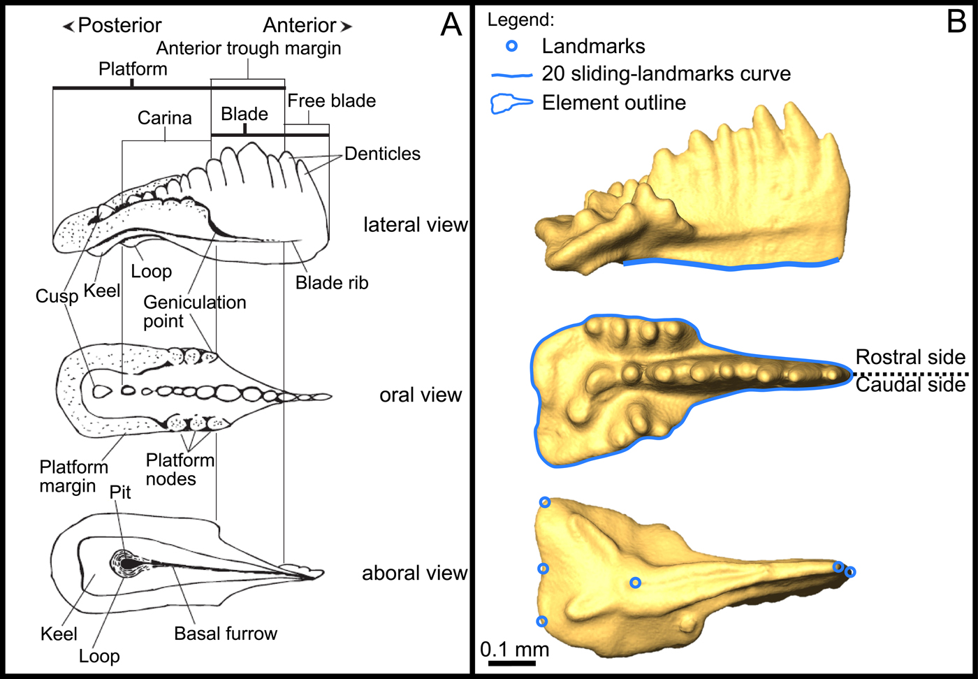
Figure 2. A, Definition of P1 morphological terms from Mazza et al. (Reference Mazza, Rigo and Gullo2012b); B, location of the landmarks used, sliding-landmarks curve, and outline. The illustrated specimen belongs to Epigondolella rigoi.
Geometric Morphometrics
A set of six landmarks was digitized on the aboral view, as well as a 20-sliding-landmark-based curve on the lower margin in lateral view, using tpsDig v. 2.30 (Rohlf and Marcus Reference Rohlf and Marcus1993; Rohlf Reference Rohlf2006) (Fig. 2B). For each data set, a generalized Procrustes analysis was performed using tpsRelw v. 1.67 (Rohlf Reference Rohlf2007). Using this method, configurations of landmarks and sliding landmarks were (1) scaled, (2) translated, and (3) rotated to minimize the sum of squared distances between corresponding landmarks. The resulting coordinates were used as shape variables for the multivariate analyses.
The outline of the element in oral view was extracted and reduced to 24 equally spaced points (origin set at the rostral geniculation point), which were used as input for an elliptic Fourier analysis (Kuhl and Giardina Reference Kuhl and Giardina1982) using the ‘Momocs’ package (Bonhomme et al. Reference Bonhomme, Picq, Gaucherel and Claude2014) in R software (R Core Team 2018). This method decomposes the outline signal into harmonics, each described by four Fourier coefficients. Here, eight harmonics were retained, which together describe 99% of the original outlines.
The potential measurement bias introduced by slightly different orientations of the pictured elements was tested, and it was found to be not significant in this study.
The three sets of variables (landmark and sliding-landmark coordinates and coefficients of outline harmonics) were summarized using principal component analysis (PCA) on variance–covariance matrices. Then the relationships between the three data sets were investigated using the STATIS method (Lavit et al. Reference Lavit, Escoufier, Sabatier and Traissac1994), which allows performing the joint analysis of K tables (one per data set, K = 3 in our case) sharing the same rows (specimens). The STATIS method is carried out in two steps (Thioulouse and Chessel Reference Thioulouse and Chessel1987; Blanc et al. Reference Blanc, Chessel and Dolédec1998). In the first step, called interstructure analysis, one searches for a compromise structure computed as the weighted sum of the K tables. Coefficients are obtained from the singular-value decomposition of the matrix of the RV coefficient, which is the multidimensional equivalent of the ordinary correlation coefficient between two variables (Robert and Escoufier Reference Robert and Escoufier1976). The corresponding eigen analysis yields factorial axes that describe the common structure across sets of variables, which is analogous to an average morphospace. During the second step, called intrastructure analysis, the projections of rows and columns of each individual data set onto the compromise axes are computed as supplementary individuals and supplementary variables, respectively. In addition, the axes of separate PCAs in each data set can be projected onto the compromise structure too, allowing for the identification of the axes of the separate PCAs best describing the common structure among the three data sets. These PCA axes are then used as shape variables. This procedure helps to minimize the number of relevant variables used in further statistical analyses. For each view, only the PCA axes that together explain at least 80% of the cumulated variance were considered. Finally, these axes were illustrated in terms of morphological variation to better visualize covariations between morphological traits. Statistical tests were performed using the ade4 (Dray et al. Reference Dray, Dufour and Chessel2007) library available in R software.
A permutational multivariate analysis of variance (PERMANOVA) (Anderson Reference Anderson2001) was performed on the STATIS compromise scores using PAST v. 3.16 (Hammer et al. Reference Hammer, Harper and Ryan2001) to test the significance of (1) the shape differences between sinistral and dextral-mirrored elements and (2) the intergeneric morphological differences. PERMANOVA may be critically sensitive to heterogeneity of variance between groups (Anderson and Walsh Reference Anderson and Walsh2013; Anderson Reference Anderson2017). As the studied groups were balanced, we avoided this problem. To assess whether the slopes of reduced major axes (RMA) of each species calculated in the STATIS compromise were significantly different, we used the χ2 test for multiple comparison of RMA slopes available in PAST. Correlation between shape variables was tested in R using the Spearman's correlation coefficient in order to account for nonnormality of these variables, and graphic representations were produced using the R package ‘ggplot2’ (Wickham Reference Wickham2016). In all analyses, α = 5%.
The data sets analyzed in this study and the lines of code we used in R are available as Supplementary Material.
Results
Main Patterns of Shape Variation
The quantification of the morphological characters of the elements was done on the three standard views. There was no significant morphological difference between dextral-mirrored and sinistral elements for each quantified character (PERMANOVA performed on aligned and harmonic coordinates, p > 0.2). Hence, the dextral-mirrored images were included in the data set and treated equally as sinistral elements in further analyses.
The three data sets were analyzed independently using a PCA. For each data set, only the most significant PCA axes explaining together at least 80% of the cumulated variance were considered.
The analysis of the lower margin in lateral view (Fig. 3A) returns two principal axes of morphological variation:
• The first axis (69.6% of explained variability, “lower margin bending”) corresponds to the flexure of the lower margin, ranging from semi-elliptic (upward bending) to “wavy” (associated with a stronger downward bending of the posterior end) for the most extreme morphotypes;
• The second axis (14.0%, “lower margin posterior dip”) highlights posterior modifications of the lower margin, with a more or less conspicuous dip of the posteriormost end of the anterior process.
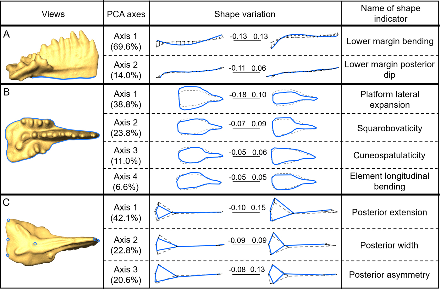
Figure 3. Selected principal components (shape variables) for each view. A, lateral view, lower margin curve; B, oral view, outline analysis; and C, aboral view, set of six landmarks. For each PCA, the percentage of explained variance is given; the extreme morphotypes are represented in solid line (associated with the corresponding score along the axis) as superimposed on the consensus shape represented in dashed line (average shape of the assemblage). The illustrated specimen belongs to Epigondolella rigoi.
The analysis of the element outline in oral view highlights four main axes of variation (Fig. 3B):
• The first axis (38.8% of explained variability, “platform lateral expansion”) corresponds to variation in the overall width of the platform.
• The second axis (23.8%, “squarobovaticity”) corresponds to variation between elements with a short (about half the length of the element), subsquared platform and elements with an obovate platform (ovate shape with tapering toward the anterior end).
• The third axis (11.0%, “cuneospatulaticity”) illustrates the variation between long wedge-shaped (“cuneate”) elements and spoon-shaped (“spatulate”) elements with a relatively short and elliptical platform.
• The fourth axis (6.6%, “element longitudinal bending”) corresponds to the overall bending and asymmetry of the element.
In aboral view, the variation of the relative position of the pit can be summarized by three principal components (Fig. 3C):
• The first axis (42.1% of explained variability, “posterior extension”) corresponds to a variation of the dimensions of the posterior end of the elements relative to the entire element: the triangle defined by the two posteriormost corners and the pit remains subequilateral or isosceles, while the size of this triangle varies between one-third and two-fifths of the element length.
• The second axis (22.8%, “posterior width”) corresponds to variation in the relative length of the posterior part, which gets slightly shorter when the platform gets relatively wider. In other words, it corresponds to lateral expansion of the posterior end of the platform.
• The third axis (20.6%, “posterior asymmetry”) illustrates variation in asymmetry of the posterior part of the element: the more asymmetrical, the shorter the posterior end; additionally, the wider side gets deflected anteriorly.
Combined Analysis of the Three Geometric Morphometrics Data Sets
To explore the overall shape variation within this assemblage and to assess the weight of each shape descriptor on the global variation, we used the STATIS method. For each view, we projected the principal components described earlier onto the three-table STATIS compromise (built on the three sets of morphometric variables), and then analyzed their relative importance using a correlation circle (Fig. 4B). The specimens of Hayashiella, Carnepigondolella, and their supposed descendants (representatives of Metapolygnathus and Epigondolella) group in two significantly distinct clusters in the STATIS compromise (PERMANOVA, p < 0.001). The axis along which these two groups are most discriminated makes an angle of about 45° with the first STATIS component (Fig. 4A, C1 = 33.5% of the total variance). Furthermore, the main axes of intraspecific variation (i.e., the major axes of each specific ellipse) do not differ significantly from one another (overall χ2 test for RMA slope comparison: χ2 = 6.0, p = 0.24), highlighting a pattern of intraspecific variation shared by all analyzed taxa (Fig. 4A). This common axis of intraspecific variation appears subperpendicular to the axis separating the two main clusters.
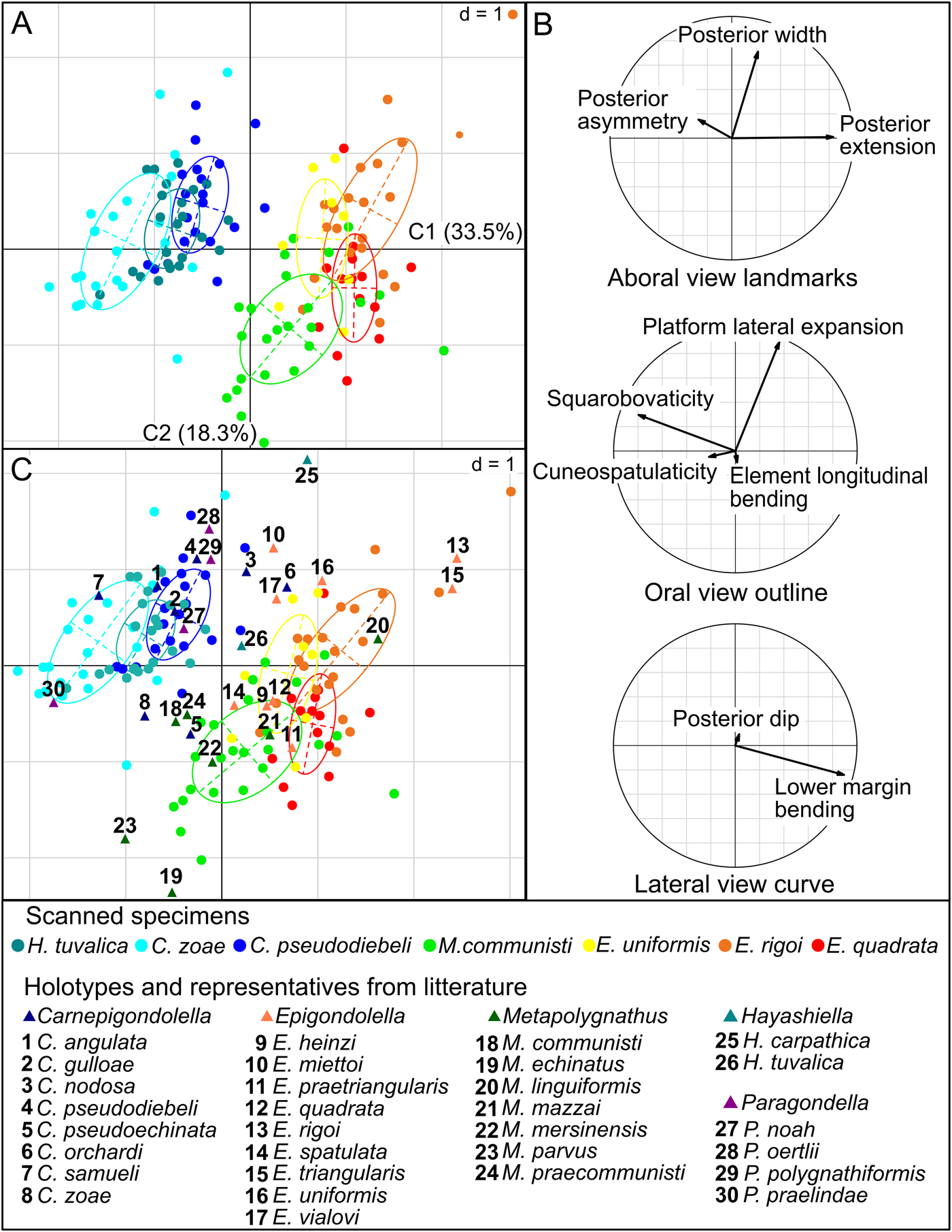
Figure 4. A, The first two axes (C1 and C2) of the STATIS compromise showing the best separation of specimens (dots) associated to the three sets of coordinates. Ellipses (63% of the specimens within a given species) identify specimens belonging to a given species (the scale “d” corresponds to the grid size). B, The first two axes of a STATIS compromise correlation circle showing the projections of the principal components of separate PCAs selected in Fig. 3. C, The first two axes of the STATIS compromise with holotypes and representatives of species included in the phylogenetic hypothesis of conodonts from the Pizzo Mondello section. Abbreviations for the legend: C., Carnepigondolella; H., Hayashiella; E., Epigondolella; M., Metapolygnathus; P., Paragondolella.
Using the correlation circles we can interpret these observations in terms of biologically meaningful, morphological parameters (Fig. 4B). On one hand, the parameters that most align with the axis separating the “Carnian” ancestors from their presumed “Norian” descendants are the lower margin bending, the squarobovaticity, and the posterior asymmetry. Note also that the nonaligned posterior extension has a greater contribution than the posterior asymmetry in the morphological transformation associated with this intergeneric axis (the projection of the corresponding arrow on the separation axis is larger than the one for posterior asymmetry). In other words, the transition from Hayashiella and Carnepigondolella to Epigondolella and Metapolygnathus in this data set corresponds, in P1 elements, to a more upward-bent lower margin, a shorter and squarer platform, and a relatively larger posterior part.
On the other hand, the platform lateral extension and the posterior width are the parameters most aligned with the common axis of intraspecific variation. This suggests that, within a given species, elements tend to show varying degrees of platform lateral expansion associated with modifications of the relative width of the posterior part: the larger the lateral expansion of the platform, the larger the posterior part (in overall size relative to element length) but the narrower the posterior part, and the more elliptic the element.
As is implicit from the patterns of variation described, most parameters are covarying to some degree. In particular, the lower margin bending, squarobovaticity, and posterior extension are significantly pairwise correlated (Spearman's correlation test, 0.57 < |ρ| < 0.74, p < 0.001; Fig. 5). Likewise, platform lateral extension and posterior width are negatively correlated (Spearman's correlation test, ρ = −0.52, p < 0.001).
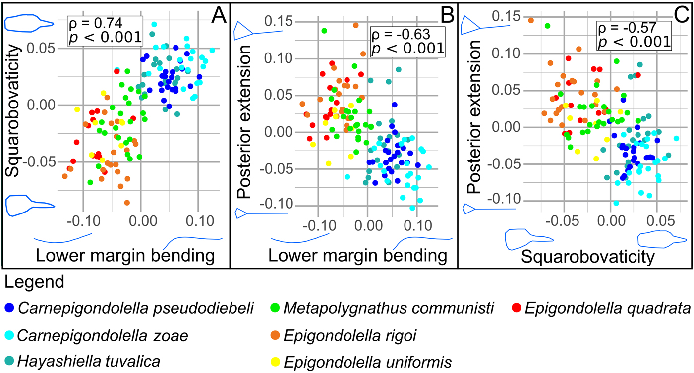
Figure 5. Correlations between A, Lower margin bending and squarobovaticity; B, lower margin bending and posterior extension; C, squarobovaticity and posterior extension. All correlations were tested by a coefficient of Spearman's correlation (ρ) and a p-value (p). Each species is associated with a single color.
As with the STATIS compromise (Fig. 4A), species are hardly distinguished from one another based on a single pair of characters: the spread of the intraspecific variation is usually much greater than the distance between the means of two given species. The distinction between the Carnian and Norian forms analyzed in this study is driven by the lower margin bending. In this data set, carnepigondolellid and hayashiellid forms tend to have a relatively longer platform that is obovate in oral view, a posteriorly located pit, and a wavy lower margin. Epigondolellid forms tend to have a relatively short platform and a large posterior end (squared), a centrally located pit, and a semi-elliptic lower margin. Metapolygnathus appears as intermediate between them for the considered descriptors.
To best represent the overall morphological variation of Paragondolella, Carnepigondolella, Metapolygnathus, Hayashiella, and Epigondolella at Pizzo Mondello, the holotypes and representatives of 30 conodont species were added to the STATIS analysis (Fig. 4C). The structure of the morphospace was found similar to the one previously described with the seven studied species only. The holotypes of the studied species fall within the range of variation of the samples, except for those of Hayashiella tuvalica, E. quadrata, and E. uniformis, which remain close to their species sample variation range. It is unclear whether this shift is due to an orientation bias introduced by using photographs from the literature produced by different authors. Paragondolella and Carnepigondolella are located in the same area, and they are separated from their supposed descendants, Epigondolella and Metapolygnathus.
Discussion
This study focused on the analysis of the morphological variation and covariation of a data set of Late Triassic (late Carnian to early Norian) P1 conodont elements. The STATIS analysis shows that the Carnian basal forms clearly differ from the Norian derived forms. On one hand, the intraspecific and intergeneric morphological variations correspond to two distinct patterns driven by characters that covary at both taxonomic levels (Fig. 6). On the other hand, the different species within each of these groups cannot be distinguished using only the morphological traits considered here.
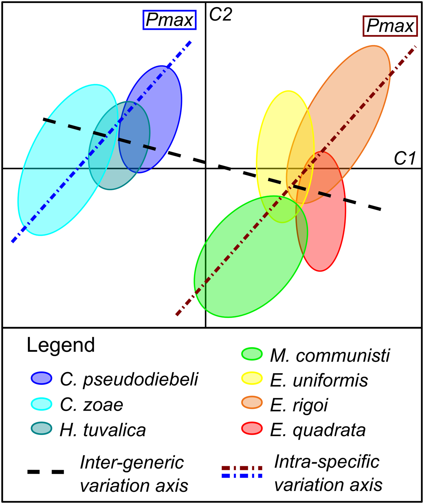
Figure 6. Illustration of the inter- vs. intraspecific patterns of variation based on the first two axes (C1 and C2) of the STATIS compromise. The ellipses identify species. C., Carnepigondolella; H., Hayashiella; E., Epigondolella; M., Metapolygnathus.
The Morphological Characters: Different Implications at Different Taxonomic Levels
Within each genus, the intraspecific variation usually overlaps in the three-table STATIS compromise. This can be due to the fact that the ornamentation of the platform and the morphology of the keel end were not quantified here, as we considered only the characters that are present in all taxa, which is not the case for platform ornamentation and the keel morphology. Nevertheless, this morphological analysis shows that: (1) a few characters are sufficient to group related species and to reveal the morphological transformations that occurred between the basal and the derived groups (i.e., the lower margin bending, the squarobovaticity, and the posterior extension, Fig. 4A); (2) the same morphological transformations were involved in the evolution of two separate lineages (i.e., parallel evolution between Carnepigondolella−Metapolygnathus and Carnepigondolella−Epigondolella; Figs. 4, 5); and (3) the characters driving variation at the intraspecific level (i.e., the posterior width and the platform lateral expansion) differ from those driving morphological variation at the intergeneric level (Fig. 4A,B).
This study highlights for the first time a common pattern of intraspecific variation within a conodont assemblage consisting of closely related taxa. All the available adult specimens that were preserved well enough to conduct the geometric morphometric analysis were considered, thus avoiding any “cherry-picking” bias. Nevertheless, the elements analyzed here represent only a portion of the available material, as the method requires fully preserved conodonts. Because the specimens had been already determined and hence classified into specific bins, the observed consistency of the intraspecific variation may correspond to a generic concept of conodont species variability, even if unlikely.
Global Environmental Disturbance as an Explanation for the Morphological Shift
The studied data set can also be used to investigate environmental versus developmental drivers of conodont evolution within the analyzed time series by using the theoretical framework of the lines of least evolutionary resistance (Schluter Reference Schluter1996; Renaud et al. Reference Renaud, Auffray and Michaux2006; Hunt Reference Hunt2007). According to this theory, species would evolve preferentially along the main axis of intraspecific phenotypic variance (Pmax). Further, any significant deviation from the Pmax trajectory can be interpreted as reflecting the influence of nonrandom selective factors such as environmental pressures.
The fact that the main intergeneric axis of phenotypic variance is almost perpendicular to Pmax in two separate lineages strongly suggests that the evolution of these Norian forms was driven by an external perturbation (Fig. 6). The location within the morphospace of the Paragondolella specimens among Carnepigondolella−Hayashiella specimens is consistent with this hypothesis (Fig. 4).
Note also that the main morphological trends between Carnian and Norian forms are observed independently of taxonomic classifications, because they were also described, with the exception of the lower-margin profile of the platform, by Orchard (Reference Orchard2014), based on similar collections from the Black Bear Ridge section in Canada, and despite a divergent view on taxonomy and phylogeny of these conodonts.
As the Pizzo Mondello section is a GSSP candidate for the definition of the CNB, detailed geochemical and paleontological studies have been already carried out (Mazza et al. Reference Mazza, Furin, Spötl and Rigo2010, Reference Mazza, Rigo and Gullo2012b), and their results can be interpreted in terms of paleoenvironments. The stable carbon isotope record (Mazza et al. Reference Mazza, Furin, Spötl and Rigo2010) of the Pizzo Mondello section shows a quasi 1‰ positive excursion at the base of the CNB interval (Muttoni et al. Reference Muttoni, Kent, Olsen, Di Stefano, Lowrie, Bernasconi and Hernández2004: Fig. 3, at 84.5 m; Mazza et al. Reference Mazza, Furin, Spötl and Rigo2010: Fig. 5, at 82 m). This approximately 1‰ positive shift coincides with the most conspicuous faunal turnover in this section: most of the carnepigondolellids go extinct and specimens of Metapolygnathus and Epigondolella become abundant (Fig. 7). A similar positive shift of δ13C along with a conodont turnover is observed around the CNB at Black Bear Ridge, Canada, on the other side of Pangea. Onoue and coworkers (Reference Onoue, Zonneveld, Orchard, Yamashita, Yamashita, Sato and Kusaka2016) interpreted this δ13C shift as resulting from anoxic conditions. Mazza and coworkers (Reference Mazza, Furin, Spötl and Rigo2010), on the other hand, interpreted the shift in Pizzo Mondello as resulting from an expansion of photosynthetically active organisms. Despite these different interpretations (note that both are not mutually exclusive), paleoenvironmental and faunal changes around CNB were not restricted to Pizzo Mondello and were likely of global extent.
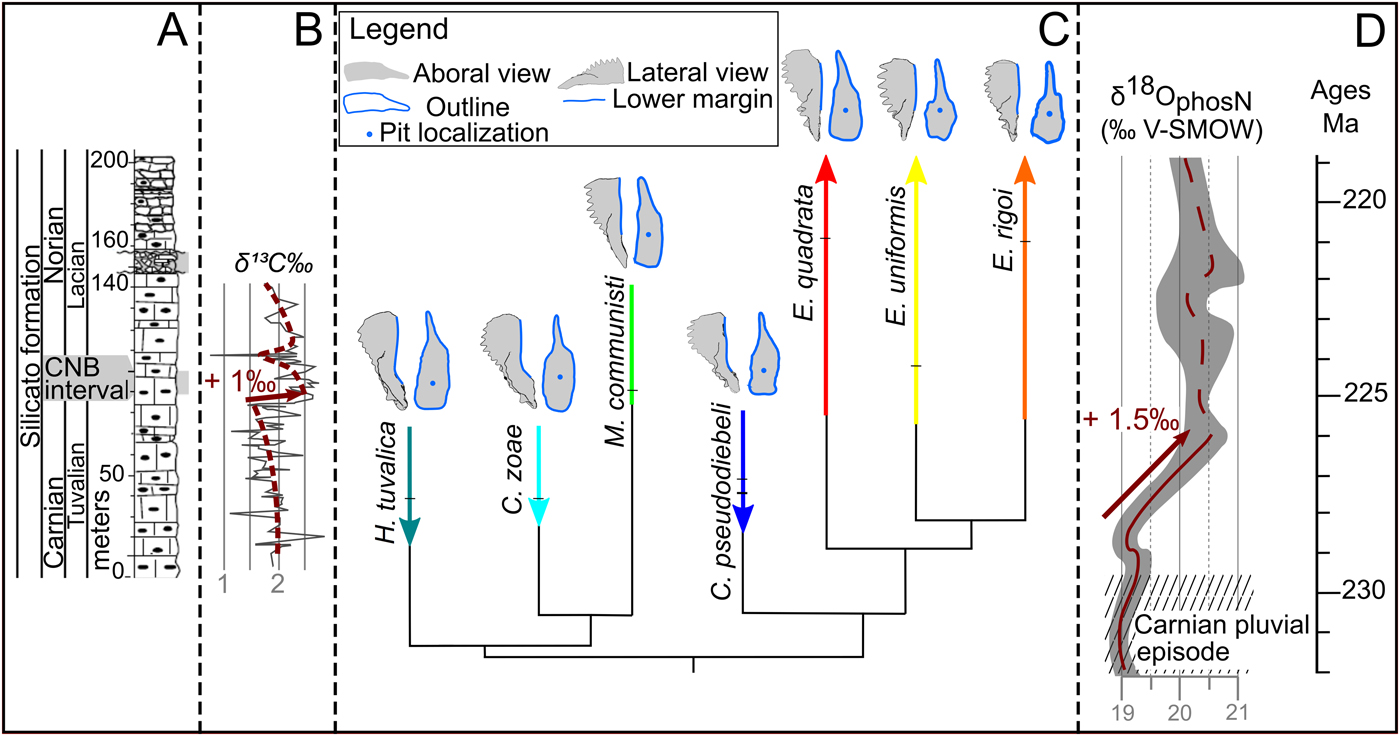
Figure 7. Synthetic illustration including sedimentologic, geochemical, stratigraphic, and morphological data of the Pizzo Mondello section and at global scale. A, Log including the Carnian/Norian boundary (CNB) interval, and a part of the upper Carnian and lower Norian (after Mazza et al. [2012a]). B, δ13C isotopic data obtained from carbonate bulk sample, including the 1‰ shift occurring just before the CNB interval (Mazza et al. Reference Mazza, Furin, Spötl and Rigo2010). The dashed line and the arrow highlight the shift (image modified after Mazza et al. [2010]). C, Global stratigraphically calibrated cladogram reduced to the seven studied species (modified after Rigo et al. [2018]). The stratigraphic range, location of the samples used in this study, and specimen consensus are represented for each species. D, Global conodont-based δ18O isotopic curve showing the 1.5‰ positive shift (modified after Trotter et al. [2015]). Absolute timing calibration was based on Kent et al. (Reference Kent, Olsen and Muttoni2017).
At the global scale, a 1.5‰ increase of the Tethyan subtropics stable oxygen isotope ratio (δ18Oapatite, measured on conodont elements) from the late Tuvalian (late Carnian) to the early Lacian (early Norian) was demonstrated by several authors (Rigo and Joachimski Reference Rigo and Joachimski2010; Rigo et al. Reference Rigo, Trotter, Preto and Williams2012; Trotter et al. Reference Trotter, Williams, Nicora, Mazza and Rigo2015), implying a decrease of 6°C in seawater temperature. This cooling followed the Wrangellian volcanism and the Carnian pluvian episode and marked a return to an arid climate. It coincided with low pCO2 values (Fletcher et al. Reference Fletcher, Brentnall, Anderson, Berner and Beerling2008) and a major faunal turnover at several trophic levels: replacement of almost all coral species (Stanley Reference Stanley1988) and emergence and radiation of new phytoplankton (dinoflagellates and coccoliths) lineages (Payne and Van de Schootbrugge Reference Payne and Van de Schootbrugge2007) and marine and terrestrial vertebrates, including dinosaurs, pterosaurs, turtles, crocodilians, and mammals (Benton et al. Reference Benton, Forth and Langer2014). This suggests a major shift in available food resources, and conodonts were likely affected by this shift. The morphological evolution of their P1 elements may thus reflect adaptations to new diets.
A Link between Shape and Function
Hitherto, no functional model has been available for the studied lineages. Yet, Martínez-Pérez et al. (Reference Martínez-Pérez, Plasencia, Jones, Kolar-Jurkovšek, Sha, Botella and Donoghue2014a, Reference Martínez-Pérez, Rayfield, Purnell and Donoghueb, Reference Martínez-Pérez, Purnell, Rayfield and Donoghue2016) analyzed different platform-bearing P1 elements using 3D models, microwear observations, and finite element analysis. For instance, they suggested that the evolution of the platform in Polygnathus may reflect an increased accommodation to biomechanical stress—in other words, a stronger bite (Martínez-Pérez et al. Reference Martínez-Pérez, Purnell, Rayfield and Donoghue2016). Extrapolating these studies to the present material, it seems likely that the P1 elements of Carnepigondolella and Metapolygnathus−Epigondolella, respectively, correspond to different occlusal mechanics (see next paragraph), a possible topic for future research.
As suggested previously (Mosher Reference Mosher1968; Mazza et al. Reference Mazza, Cau and Rigo2012a), the transition from Carnian to Norian forms involved modifications of the lower-margin profile of the platform (captured in the lower margin bending principal component), a shortening of the platform relative to the entire element (see brevicuneoellipticity and posterior extension principal components), and a shifting of the pit (i.e., a relative enlargement of the posterior part of the element; see posterior extension) (Figs. 7, 8). Moreover, even if it was not quantified here, the ornamentation of the platform became more complex, showing a development from nodes restricted to the middle and anterior parts of the platform (Carnian) to nodes or denticles all over the platform (Norian) (Mazza et al. Reference Mazza, Cau and Rigo2012a). The combination of a wavy baseline and a poor platform ornamentation (Carnepigondolella group) may reflect a rotational movement of the P1 elements, whereby occlusion starts in the anterior part of the element with a blade-to-blade contact (which may have functioned as an occlusional guide or as a cutting device) and ends in the posterior part with a platform-to-platform contact that was likely used for crushing food items. On the other hand, the combination of a semi-elliptic baseline and a strong platform ornamentation (Epigondolella species) suggests a translational movement of the P1 elements toward one another and a direct occlusion between the sharp platforms that may have been used for perforation and ripping of the food items.
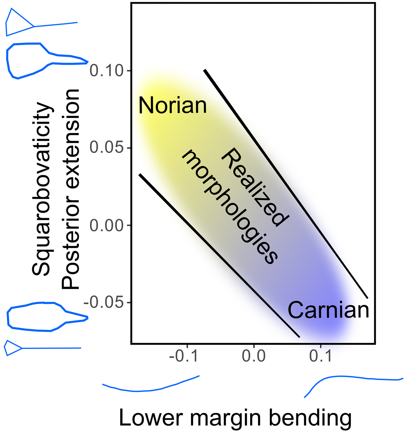
Figure 8. Illustration of the constrained morphologies of the conodont elements through the Carnian/Norian interval.
The Developmental Mechanisms under the Evolutionary Shift
The fact that the very same evolutionary path was followed in two presumably distinct lineages in the Pizzo Mondello section suggests that the morphologies of these two lineages were constrained in a similar way, and possibly by the same drivers. Beyond the patterns of intraspecific and intergeneric variation, the correlations we demonstrated between, on one hand, the lower margin bending, squarobovaticity, and posterior extension (and, implicitly, platform ornamentation), and on the other hand, the posterior width and platform lateral expansion also emphasize the existence of “restricted” areas in the morphospace for which no realized morphology is observed (Fig. 8; see also Fig. 5). As far as P1 conodont elements are concerned, this suggests that general laws of covariation exist that apply not only within species, but also at higher taxonomic levels. These laws may be the consequence of some developmental and/or functional constraints. For instance, the association of a wavy baseline and a large posterior platform (and/or a highly ornamented platform) is never observed in this assemblage. While different observed morphological associations may reflect different feeding mechanisms (see “A Link between Shape and Function”), nonobserved associations may correspond to morphologies that are either developmentally “impossible” or functionally “nonviable,” because they could prevent proper occlusion and hence proper feeding.
The effect of environmental changes has often been at the core of evolutionary studies in deep time, whereas the developmental aspects of the considered organisms have often been neglected. Inferring developmental constraints from the fossil record is not an easy task, but as we have shown, it is not an impossible one (see also Ciampaglio Reference Ciampaglio2002; Moulton et al. Reference Moulton, Goriely and Chirat2012; Urdy et al. Reference Urdy, Wilson, Haug and Sánchez-Villagra2013; Erlich et al. Reference Erlich, Moulton, Goriely and Chirat2016). Paleo-eco-evo-devo studies are thus feasible and are likely, in the near future, to tremendously enhance our understanding of the evolutionary processes that shaped and are shaping life.
Conclusion
A parallel evolutionary path between two lineages, highlighted by a common pattern of intraspecific and intergeneric variation, suggests the existence of generic laws of morphological trait covariation in conodont elements. The transition between Carnian forms and their presumed Norian descendants corresponds to an axis in the morphospace that is very different from the axis of intraspecific variation affecting all pre- and post-CNB species, suggesting that the intergeneric evolution of these elements did not follow the expected evolutionary path of least resistance. This may reflect the consequences of an environmental disturbance, as emphasized by the carbon and oxygen stable isotope records during that particular interval, and/or its ecological implications for conodonts, such as a possible diet change. This would have constituted a selective pressure on the shapes of conodont elements. The present study is a first step toward a general quantification and better understanding of the patterns of variation and covariation in euconodonts, and hence a better interpretation of their morphological evolution. Thanks to their ~300-Myr-long, widespread abundance in marine strata, conodont elements appear to be a very useful model to study evolutionary processes in deep time.
Acknowledgments
We thank Mathilde Bouchet (ENS Lyon, SFR Biosciences) for her invaluable help with the microtomography and Gilles Escarguel (Université Lyon 1) for his advice on statistics. Gilles Escarguel is also thanked for having discussed several drafts of this article. Finally, we thank Emilia Jarochowska, Carlos Martínez-Pérez, and an anonymous reviewer who corrected the draft and helped to improve this article. This research is supported by a French ANR @RAction grant to N.G. (ACHN project EvoDevOdonto).


