


1. GIOVE MISSION OVERVIEW
The Galileo System Test Bed second generation (GSTB-V2) or Giove Mission is supporting the early Galileo mission (GSTB-V1) experimentation in critical areas, in order to mitigate programmatic and technical risks of the Galileo In Orbit Validation (IOV) phase. The phases are outlined in Figure 1. The work concentrates mainly on the on-board clocks characterization, the Signal In Space experimentation, the Galileo navigation algorithms validation and the characterization of the Galileo Sensor Stations performances. The main purpose of the GSTB-V2 mission is to transmit all the types of Galileo navigation signals and validate receiver performance and assess environmental effects [Reference Hahn2].

Figure 1. Galileo mission phases.
The GSTB-V2 system consists of three elements:
• the Ground Control Segment (GCS);
• the Ground Mission Segment (GMS);
• the Space Segment.
In the GCS there are two control centres. Each control centre manages control functions, supported by a dedicated GCS, and mission functions which are supported by a dedicated GMS. The core of the ground mission segment is the network of the Galileo Experimental Sensor Stations (GESS), consisting of 13 stations placed around the world (See Figure 2). Eleven GESS stations are connected to the Data Server Facility (DSF) through Sensor Station Data Servers (SSDS); seven stations are managed by the European Space Operations Centre (ESOC), four are managed by Geo Forschungs Zentrum (GFZ), two stations are directly connected to the DSF, one is managed by Istituto Elettrotecnico Nazionale (IEN) and one by the GSTB Processing Centre (GPC) [3].

Figure 2. GSTB v2 GESS locations.
The GESS continuously acquire the GIOVE SIS (Signal in Space) and the Global Positioning System (GPS) L1/L2 signals throughout the orbit revolution. Each GESS stations includes a Galileo Experimental Test Receiver (GETR), a dual-constellation multi-frequency receiver, with six generic Galileo/GPS channels, one Alternative Binary Offset Carrier (AltBOC) channel, and nine dual-frequency (L1&L2). These channels are fully flexible and can be assigned to different Galileo and GPS satellites. Alt-BOC modulation can be represented as an 8-PSK (Phase Shift Keying) Signal Phase Angle (1 to 8) determined from binary values of the four coherent E5 codex data streams [Reference Plriz, Tavella and Giraud.15]. The GETR can operate in dual constellation GPS/Galileo mode and in single constellation.
The other components of the GESS are: a Galileo Reference Antenna, an Industrial PC (Core Computer) allowing data collection and storage, a modem or a front-end providing the network access point necessary to link GESS and DSF (located at the GPC), an Uninterruptible Power Supply (UPS), which allows the station to operate 90 minutes without electrical energy and a Low Cost Portable Frequency Rubidium Standard.
Two GESS models are available: Standard GESS (S-GESS) using its built-in frequency standard based on a Low Cost Portable Frequency Rubidium Standard and GESS for Timing Laboratories using the frequency standard provided by the site. GESS performance is declared satisfactory when the expected figures of merit are obtained by the Sensor Stations Characterization (SSCh) and the data can be processed. Consequently, according to the planned SSCh analysis, the following performances are considered key parameters, and contribute to the definition of “performance targets”:
• GESS Operational status: GESS shall be able to steadily reach the nominal tracking status, i.e. “code and phase loops locked”, so that it is able to deliver observables to DSF.
• Data availability: GESS shall be able to provide code and phase measurements with 50% availability for periods when satellite elevation is above 10°. In order to be significant, reasonable data availability is necessary.
• Data continuity: GESS shall be able to provide code and phase measurements with no more than 1 data gap per 30 minutes.
• Cycle slip occurrence: GESS shall be able to provide code and phase measurements with no more than 1 cycle slip per 30 minutes. Indeed, key SSCh algorithms need 10 minutes of consecutive measurements with no gap and no cycle slip in order to be able run.
• Blanking device operation: GESS shall operate with blanking ON in order to carry out experimentation on blanking statistics [Reference Plriz, Tavella and Giraud.15].
In navigation, clocks are the driving factor for determining positions accurately. ESA has chosen to use a Rubidium Atomic Frequency Standard (RAFS) and Passive Hydrogen Maser (PHM) on the satellites; the stability of the RAFS is so good that it would lose only three seconds in one million years, while the PHM is even more stable and it would lose only one second in three million years. This precision is related to the clock's stochastic noise, however its deterministic error (frequency offset and drift) would cause larger errors in time. An atomic clock works like a conventional clock but the time-base of the clock, instead of being an oscillating mass as in a pendulum clock, is based on the properties of atoms when transitioning between different energy states. An atom excited by an external energy source goes to a higher energy state, from current state, and later it comes back to a lower energy state. In this transition, the atom releases energy at a very precise frequency, which is characteristic of the type of atom [Reference Jeanmaire, Rochat and Emma16]. The development of the RAFS started at the end of 2001 and was completed at the beginning of 2003 with the delivery of an Engineering Model (EM), which is the baseline unit for the development of the flight models for GSTB-V2 [4].
Two test satellites, GIOVE A and GIOVE B – Galileo IOV Element – are currently in orbit. They were launched to:
• Secure use of the frequencies allocated by the International Telecommunications Union (ITU) for the Galileo System;
• Characterize the orbits to be used by the In-Orbit validation satellites;
• Characterize the On-board clock (RAFS and PHM, the most precise GNSS clock in space ever) technology in space;
• Collect lessons learned on Space Segment onboard units pre-development and in-orbit operations;
• Provide early demonstration and performance assessment of the navigation service (including navigation message uplink and broadcast);
• Facilitate overall testing of timelines and operational aspects (including data collection from GESS), data processing, message generation and uplink.
Both satellites transmit the navigational signals that will be used by Galileo when it becomes operational.
2. STATISTICAL BACKGROUND
Within the GIOVE navigation system, the block used in signal transmission can be seen as a communication system. The theory of probability and stochastic processes is an essential mathematical tool in the study of communication systems. Many of the random phenomena that occur in nature are functions of time: also the thermal noise that is generated on the resistance of electronic devices such as a GIOVE receiver can be seen as a function of time.
Instead of dealing with only one possible “reality” of how the process might evolve under time (as is the case, for example, for solutions of differential equations) in a stochastic or random process there is some indeterminacy in its future evolution described by probability distributions. This means that even if the initial condition (or starting point) is known, there are many possibilities the process might go to, but some paths are more probable than others.
So at any given epoch, the value of a stochastic process, whether it is the value of the noise voltage generated by a resistor or the amplitude of a signal received by a GIOVE receiver, is a random variable. Thus, it is possible to consider a stochastic process as a random variable indexed by time parameter t. The noise voltage generated by a single resistor represents a single realization of the stochastic process. GIOVE measurement errors are dominated by the systematic errors caused by the orbit, atmospheric and multipath effects, which are quite different for each satellite. Therefore, the measurements obtained from the two satellites cannot have the same precision [Reference Gaglione, Angrisano, Pugliano, Robustelli, Santamaria and Vultaggio6].
On the other hand, the raw measurements are spatially correlated due to similar observing conditions for these measurements. This type of correlation is generally called ‘spatial correlation’. Moreover, the time correlations (or temporal correlations) may exist in the measurements because the residual systematic errors change slowly over time.
To analyze GIOVE satellite pseudorange error we can chose from the following independent variables: satellite elevation, Signal-to-Noise Ratio (SNR) or least-squares residual [Reference Satirapod5].
2.1 Elevation
Satellite elevation angle information is often used to study pseudorange error. The basic assumption of using the satellite elevation angle information is that each satellite has a different precision and it is assumed that a low elevation angle satellite tends to be noisier than a high elevation angle one. The relationship between satellite elevation angle information and precision can be modelled quite well by a decreasing exponential function.
2.2 Signal-to-Noise Ratio (SNR)
Recently, SNR was introduced as a quality indicator for GPS observations and used to study pseudorange error. The basic assumption is that each satellite has a different precision which is dependent on the SNR information. A satellite with a high SNR value will be less noisy than one with a low SNR value. Langley (1997) [Reference Langley7], claims that SNR is the key parameter in analyzing GPS receiver performance and that it directly affects the precision of GPS observations.
2.3 Least-Squares Residual
The basic assumption is that residuals obtained from the least-squares process would represent the same characteristic as true errors if the observation period is long enough to remove any systematic error. Thus, the precision of each satellite is dependent on the residuals obtained from the least-squares process. Based on the use of least-squares residuals, many rigorous statistical methods, i.e. MINQUE [Reference RAO8] or Bayes estimation [Reference Ziqiang9], have been used to estimate a more realistic covariance matrix.
From these possible approaches, the first option was chosen, namely the dependence by elevation.
The pseudorange error is defined as:
with d geometric distance and ρ pseudorange.
Assuming that a transmitting satellite and a receiver are fixed in space, the geometric distance d is a constant. Although in these hypothetical conditions, the error Δ is not a constant but will vary. The error is a function of effects that are not deterministic but random such as the twinkling of the ionosphere, the multipath etc. For this reason Δ will be treated as a random variable. However, the hypothesis of fixed satellite is not plausible. Removing it, the satellite position will change over time. Hence it is necessary to add the time variability to the random variable Δ, transforming it in a stochastic process. So the error on pseudorange can be modelled as a stochastic process:
where ξ is an element of sample space.
3. COMPUTATION OF PSEUDORANGE ERROR
In order to compute GIOVE pseudorange error, ESA authorized real data taken from GESS stations are used. For this purpose, GPS and Galileo navigation and observation files are used and all their real time information are considered in order to apply the proper correction to the raw pseudorange (e.g. the satellite clock correction computed starting from the broadcast parameters).
The pseudorange error computation is the core of this work; to assess its features, it is necessary to remove all the deterministic errors. The raw pseudorange error is defined as:
where: ρ is the unprocessed pseudorange measurement; d is the geometric distance receiver-satellite which is computed as:
where: (X R, Y R, Z R) are the receiver coordinates (well known because the receiver is fixed and previously geo-referenced); (X SE, Y SE, Z SE) are the satellite coordinates (computed from RINEX navigation files) both in ECEF WGS84 reference system. The pseudorange measurement, stored in the RINEX observation files, is corrected for the satellite clock error, for relativity effects, for Sagnac Effect and atmospheric delays according to the equation:
where: ρ CE is the Galileo corrected pseudorange measurement; dt SatE is the satellite clock bias including TGD (Time Group Delay); dt rE is the relativistic effect correction term; dt SagE is the delay due to the Sagnac Effect; d IonoE is the ionospheric delay; d TropoE is the Tropospheric delay; dT RecE is the receiver clock bias between GIOVE time scale and the receiver one.
In order to compute the last bias a combined navigation algorithm is developed and described in next section.
4. COMBINED PVT ALGORITHM
To estimate dT RecE, a further unknown has to be included along with three position coordinates. Due to few available observations, it is not possible to compute this unknown using only Galileo satellites but a combined algorithm has to be performed. In this work a GPS/Galileo PVT (Position Velocity and Time) model is developed and described below.
The equation model is obtained by the linearization of the equation (5) and the GPS measurement one that is:
Equation (6) is formally identical to (5) and the only difference is the superscript G representing the GPS system (the superscript E is for Galileo).
The linearized observation equation can be defined as:
where: Δ ρ (m×1) is the difference vector between the m raw pseudoranges and a priori information (with m number of GPS and Galileo observations); H is (m×5) design matrix; ΔX (5×1) is the unknowns vector; ε is the residuals vector which includes all unmodelled errors (measurement noise, multipath and so on).
The explicit forms of H and ΔX are:
![$$H = \left[ \openup 8pt{\matrix{ {\displaystyle{{x_0 - x^{G1}} \over {\rho _0^{G1}}}} & {\displaystyle{{y_0 - y^{G1}} \over {\rho _0^{G1}}}} & {\displaystyle{{z_0 - z^{G1}} \over {\rho _0^{G1}}}} & 1 & 0 \cr {...} & {...} & {...} & {...} & {...} \cr {\displaystyle{{x_0 - x^{Gn}} \over {\rho _0^{Gn}}}} & {\displaystyle{{y_0 - y^{Gn}} \over {\rho _0^{Gn}}}} & {\displaystyle{{z_0 - z^{Gn}} \over {\rho _0^{Gn}}}} & 1 & 0 \cr {\displaystyle{{x_0 - x^{E1}} \over {\rho _0^{E1}}}} & {\displaystyle{{y_0 - y^{E1}} \over {\rho _0^{E1}}}} & {\displaystyle{{z_0 - z^{E1}} \over {\rho _0^{E1}}}} & 0 & 1 \cr {...} & {...} & {...} & {...} & {...} \cr {\displaystyle{{x_0 - x^{Er}} \over {\rho _0^{Er}}}} & {\displaystyle{{y_0 - y^{Er}} \over {\rho _0^{Er}}}} & {\displaystyle{{z_0 - z^{Er}} \over {\rho _0^{Er}}}} & 0 & 1 \cr}} \right]$$](https://static.cambridge.org/binary/version/id/urn:cambridge.org:id:binary:20151022042206496-0160:S0373463311000270_eqn8.gif?pub-status=live)
where the superscripts n and r are respectively the number of GPS and Galileo simultaneous measurements and ρ 0i the a priori pseudoranges (i=G,E) [Reference Cai and Gao18].
With this approach two separate receiver clock offsets are introduced with respect to GPS and Galileo system times respectively whereas the inter-systems bias (GGTO – Galileo to GPS Time Offset) is the difference between these two offsets. An alternative approach (not used in this work) consists of performing a GPS-only PVT solution to retrieve the bias between the receiver clock and the GPS system time and using the GGTO values contained in the Galileo navigation message. This last approach is not used because, as stated in ESA GIOVE A-B ICD, the GGTO fields of the navigation message(s) are being used for experimental purposes and they can not be used for positioning or timing services [19].
Equation (7) is solved for ΔX by means of Least Square (LS) method and the solution is given by the equation:
where: R (n×n) is the pseudorange error covariance matrix.
All pseudorange errors are considered independent with equal variances; so R is set equal to identity the matrix and the equation becomes:
The LS estimation is used to update the a priori value:
To be able to solve the equation (7), at least five simultaneous measurements are necessary and at least one Galileo observation should be included. When only one GIOVE satellite is tracked, the term absorbs all errors in the range measurements and so it results in more noise. In order to solve this problem the LS solution, computed each time at least one GIOVE satellite is tracked, is performed processing the less noisy P code pseudoranges. The standard deviation trend of the final Δ(cdT RecE) evaluation (which will be seen in Figure 8) shows that the result precision is about 1·25 m. This algorithm as described is shown in Figure 3 in which it can be seen that the GPS and Galileo pseudoranges are corrected in accordance with equations (5) and (6); for both the Hopfield model is used in order to correct the tropospheric delay. For the ionospheric delay, the Klobuchar model is adopted for the GPS system and the NeQuick model is applied for Galileo.

Figure 3. Combined PVT algorithm.
NeQuick is a three-dimensional and time dependent ionospheric electron density model developed at the Aeronomy and Radiopropagation Laboratory of the Abdus Salam International Centre for Theoretical Physics (ICTP) of Trieste, and at the Institute for Geophysics, Astrophysics and Meteorology of the University of Graz [Reference Radicella, Nava and Coisson20]. This model, starting from the Effective Ionization Level A z is able to provide Galileo satellite radio signal group time delay.
GIOVE-A/B provides, in the navigation file, the model parameters a 0, a 1 and a 2 used to compute the Effective Ionization Level A z, by the equation:
where μ is the Modified dip (inclination angle of local Earth magnetic field) latitude.
4. PSEUDORANGE ERROR COMPUTATION
Once the combined PVT algorithm provides the estimated dT RecE it is possible to compute the corrected GIOVE pseudorange error ΔC, defined as:
The correction procedure is shown in Figure 4.

Figure 4. Pseudorange Correction Procedures.
5. ANALYSIS AND RESULTS
Data used for this analysis covers the 24 hours of day 284 in year 2010 and are stored in GMIZ station placed in Misuzawa (Japan) in RINEX (Receiver Independent Exchange Format) format (version 3.00) with 1 Hz acquisition frequency. In this RINEX version, the data structure has been modified and the limitation of 80 characters length for the observation files has been removed; meanwhile Galileo navigation message content is very similar to GPS one (i.e. the orbit parameterization is Keplerian). The results are shown in Figures 5 and 6.

Figure 5. GIOVE A. Pseudorange error (left), histogram (right).
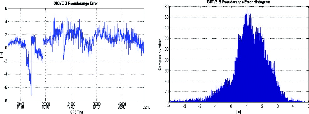
Figure 6. GIOVE B. Pseudorange error (left), histogram (right).
The GIOVE satellites (A or B) pseudorange error is characterized by a small mean (0·93 metres for GIOVE B and 0·24 metres for GIOVE A). Only in the GIOVE B trend (see Figure 6 (left)) is there a spike error of −7·22 m. In order to investigate the origin of the spike, Figure 7 shows the same plot but with a different time scale, and it is compared with relative accuracy in the evaluation of the receiver clock bias to GPS scale and Galileo.

Figure 7. GIOVE B. Pseudorange error, cdT RecE and cdT RecG accuracy.
Corresponding with the Pseudorange error of −7·22 metres the receiver clock bias to GPS time scale (cdT RecG) is evaluated with a bad accuracy. This term is one of the most important corrections to the raw GPS pseudorange (see equation 6) used in the LS method in order to compute cdT RecE.
The cdT RecE accuracy is good for the whole observation period as shown in Figure 8. A large error in the GPS system has a big influence on the final cdT RecE evaluation, and consequently on GIOVE satellite pseudorange error, due to the greater number of GPS measurement equations in the combined PVT algorithm.

Figure 8. cdT RecE accuracy.
6. FUTURE WORK
The results obtained demonstrate the consistency of GIOVE satellites performance with existing GPS and GLONASS systems. This Galileo pseudorange error assessment is to be considered as the first step for the building of a stochastic error model. Further tests must be conducted and more data must be processed to obtain more meaningful results.
ACKNOWLEDGMENTS
The authors wish to acknowledge the many valuable contributions made by ESA for the GIOVE-M data access, as well as the Eng. M. Cosmo (ASI Agenzia Spaziale Italiana) for his support and encouragement.


