


1. Introduction
As part of their effort to promote environmental protection and reduce poverty, international donors, non-profit organizations (NPOs) and governments have invested in the development and introduction of new technologies in developing countries. To accelerate the adoption of these technologies and because of the positive externalities they provide, they have been aggressively subsidizing and distributing them to broadly targeted populations. For instance, over the past couple of years the Cereal Systems Initiative for South Asia (CSISA) has put substantial effort into promoting agricultural technologies in South Asia's Indo-Gangetic Plains, such as zero-tillage, laser land leveling and early sowing of wheat, in order to improve cereal production growth and protect the environment. The adoption of these technologies, however, continues to be low and varies between different regions (Laxmi et al., Reference Laxmi, Erenstein and Gupta2007). There is growing concern over this low rate of adoption, and thus increasing the rate of utilization of new technologies is a challenge for donors (e.g., Hanna et al., Reference Hanna, Duflo and Greenstone2012; Dupas, Reference Dupas2014). This paper develops a conceptual framework to analyze the phenomenon of underuse of new technologies in the context of economic development, and to suggest marketing tools to enhance utilization and reduce waste. It borrows from a large literature in marketing that emphasizes the role of consumer fit-risk in the underutilization of products, and analyzes the role of marketing tools like money back guarantee (MBG) and demonstration in reducing fit-risk and enhancing efficiency (Heiman et al., Reference Heiman, McWilliams and Zilberman2001).Footnote 1
The economics literature on technology adoption has investigated the adoption behavior from various aspects such as production (yield) risk (e.g., Koundouri et al., Reference Koundouri, Nauges and Tzouvelekas2006; Giné and Yang, Reference Giné and Yang2009), learning (e.g., Edmondson et al., Reference Edmondson, Winslow, Bohmer and Pisano2003; Straub, Reference Straub2009), reference price (e.g., Heffetz and Shayo, Reference Heffetz and Shayo2009) and network (e.g., Katz and Shapiro, Reference Katz and Shapiro1986; Bandiera and Rasul, Reference Bandiera and Rasul2006). Yet there has been much less recognition of the existence and implications of fit-risk (Zilberman et al., Reference Zilberman, Zhao and Heiman2012).
Fit-risk occurs when potential adopters are not sure if the technology will fit their needs, lifestyles, social feedback or capabilities. Fit-risk arises because of individual-level idiosyncratic differences in local population; a technology may suit different individuals differently due to factors such as the heterogeneity of population characteristics, skills, preferences and environments. For example, people with allergies may not find technologies involving chemical application suitable to use. Fit-risk also depends on the nature of the technology and individuals who consider it. For example, adoption of tractors or vehicles for farming may depend on the capability of farmers to drive. Similarly, individuals with poor vision or observation capacity may have high fit-risk regarding an IPM strategy based on monitoring pest populations.
New technologies tend to be more efficient but also add new sources of risks, and these risks may be exacerbated because of local conditions.Footnote 2 For example, high yielding seed varieties may perform very well in the presence of irrigation and other complementary inputs, but may fail in their absence. Fit-risk, however, is inherently different from these other risks as it manifests at an individual level and differs across individuals within the same population in the same local environment. There may be complementarities between other risks associated with a new technology and fit-risk; a technology with a lower overall risk may also have a lower fit-risk. In this paper, we abstract from these complementarities and assume that the net benefit from technology takes into account the risks associated with it.
Furthermore, fit-risk is not a case of asymmetric information, because the fit of the product prior to the user experience is random and unknown both to the user and the technology provider. Not recognizing fit-risk will result in a different type of inefficiency from that caused by traditional price and quality risk, or cases of asymmetric information.
Fit-risk is especially likely to occur with experience goods, where acceptance and utilization of the good cannot be predicted with certainty unless the user experiences it. People may learn about fit-risk through alternative instruments such as social networks or learning from others. Fit-risk may also be affected by factors such as the way in which a product is packaged and/or explained. However, because fit-risk arises due to individual-level idiosyncratic differences in the local population, instruments such as social information (word of mouth), learning from others and advertisement are not sufficient to address it (Klein, Reference Klein1998).
The international development community has been exploring how private sector management frameworks are relevant for the repositioning and practicing of NPOs (e.g., Austin, Reference Austin2000; Lindenberg, Reference Lindenberg2001; Eikenberry and Kluver, Reference Eikenberry and Kluver2004). The present paper aims to develop a framework to answer this question. It identifies situations in which lack of consideration of fit-risk may result in suboptimal outcomes in technology provision by public and non-profit organizations, and how demonstration can improve market outcomes.
The analysis uses a simple threshold adoption model, which recognizes heterogeneity among potential adopters (e.g., Zilberman et al., Reference Zilberman, Zhao and Heiman2012) to derive demand for a new technology. Only those potential adopters whose expected benefit is higher than the market price will buy it. This results in inefficient non-adoption because the expected benefit drops in the presence of fit- risk. Among those who buy the technology, only those for whom the technology is suitable will use it. Thus, fit-risk may not only decrease technology adoption but also generate resource waste. Ignoring fit-risk, or misunderstanding the dynamics of technology demand under the existence of fit-risk, can lead to a miscalculation of project values and potential benefits of marketing efforts in development projects. Project donors and managers may develop different policy strategies based on the level of technology fit and cost of marketing efforts. This paper analyzes when it is worth it to incur costly demonstration of the technology that eliminates fit-risk, and shows that: (i) the economic net benefit of costly demonstration is non-monotone in the probability of fit; and (ii) demonstration is not worth it when the probability of non-suitability of the technology is either too high or too low.
Marketers in developed countries have been using MBG and demonstration to address fit-risk. While MBG is a marketing tool that allows consumers to receive some, or all, of their payment back if the purchased product does not meet their expectation and is returned within a given period of time (Heiman et al., Reference Heiman, McWilliams and Zilberman2001), demonstration is a tool that allows the consumer to experience the product before purchase. We focus on demonstration as compared to MBG since demonstration requires lower transaction costs (in terms of processing returns and reusing returned products) and does not require a great level of trust between sellers and buyers. Demonstration increases the precision of technology provision in development projects by revealing personal levels of technology fit and potential product benefits. The marketing literature finds that demonstration reduces the potential customers’ resistance and affects consumers’ prior beliefs about the product (Scott, Reference Scott1976; Roberts and Urban, Reference Roberts and Urban1988). The following examples illustrate how demonstration can help in alleviating fit-risk in new technologies. Test driving of cars is a form of demonstration that helps individuals know if a specific car appeals to them in terms of performance and convenience. The adoption of agricultural technologies, such as integrated pest management (IPM), seed transplantation, zero tillage, drip irrigation, tractors and mechanized harvesters, may be reduced without adequate demonstration.
The rest of the paper is organized as follows. Section 2 presents the model. Section 3 discusses an optimal subsidy in the presence of fit-risk, while section 4 constructs a demonstration gain function. Section 5 analyzes a policy that combines demonstration and optimal subsidy to eliminate fit-risk. In section 6, we discuss some extensions of our analysis, and finally, section 7 concludes.
2. Model
Suppose a donor wishes to introduce a technology that has the potential to improve welfare in a developing country. Private benefits derived from the technology differ across individuals in the local population – some people are likely to benefit more from the technology than others. The technology adoption delivers social value in addition to private benefit. The additional social value could be an environmental or health externality, philanthropic services of the donor, redistribution, and so forth. The technology, however, may not be suitable for all, and provides benefits only if it is suitable. Further, prior to acquiring the product, the potential beneficiaries do not know whether it will fit them. They may eventually learn about their fit after acquiring and trying it. Not knowing ex ante whether a technology will fit an individual or not is termed as ‘fit-risk’ in our model.
Assume that the private benefit from the technology, b, varies across the population of measure 1 with a continuous density function
 $f\lpar b\rpar $
and cumulative distribution function (CDF) F(b) with supports
$f\lpar b\rpar $
and cumulative distribution function (CDF) F(b) with supports
 $\lsqb \underline{b},\bar{b} \rsqb $
.Footnote
3
Suppose that the probability that the technology fits a particular individual with private benefit b is q. For simplification, we assume that q is independent of b, and is known.Footnote
4
Thus q proportion of the consumers buying the product will actually use it, and
$\lsqb \underline{b},\bar{b} \rsqb $
.Footnote
3
Suppose that the probability that the technology fits a particular individual with private benefit b is q. For simplification, we assume that q is independent of b, and is known.Footnote
4
Thus q proportion of the consumers buying the product will actually use it, and
 $\lpar {1-q}\rpar $
of the acquired products will be wasted. The expected benefit to an individual with private benefit b from adopting the technology is qb. In addition to the private benefit, the technology also has social value, v. The demand is determined by the mass of consumers for whom the expected benefit from acquiring the technology is larger than the unit cost. We also assume that each individual buys at most one unit of the technology. The quantity purchased, Q, is given by
$\lpar {1-q}\rpar $
of the acquired products will be wasted. The expected benefit to an individual with private benefit b from adopting the technology is qb. In addition to the private benefit, the technology also has social value, v. The demand is determined by the mass of consumers for whom the expected benefit from acquiring the technology is larger than the unit cost. We also assume that each individual buys at most one unit of the technology. The quantity purchased, Q, is given by
 $$Q=\int_{b^{\ast }}^{\bar{b}} f\lpar b\rpar db=1-F\lpar {b^{\ast }} \rpar ,$$
where b* denotes the marginal consumer indifferent between purchasing and not purchasing. We can analyze the quantity purchased under different scenarios by identifying the marginal consumer. For a given probability of fit q and price p, Footnote
5
the marginal consumer indifferent between buying and not buying is
 $b^{\ast }={{p}\over{q}}$
. Thus, we can define
$b^{\ast }={{p}\over{q}}$
. Thus, we can define
 $$Q\lpar {p,q} \rpar =\int_{p\over q}^{\bar{b}} f(b)db=1-F\left({p\over q} \right).$$
To understand the inefficiencies caused by fit-risk, we compare the above demand with the potential demand if there were no fit-risk. In the absence of fit-risk, the expected benefit of the technology to an individual is b. The marginal consumer indifferent between buying and not buying the technology, thus, is given by b*=p. Since the technology fits to q proportion of the population, potential demand in the absence of fit-risk,
 $\bar{Q}$
, is given by
$\bar{Q}$
, is given by
 $$\bar Q\lpar {p,q} \rpar = q \int_p^{\bar{b}} \; f(b)db = q\lpar {1 - F\lpar p \rpar } \rpar .$$
The difference between the potential demand in the absence of fit-risk and in its presence is given by
 $$\bar{Q}\lpar {p, q} \rpar - Q\lpar {p,q} \rpar = q\lpar {1 - F\lpar p \rpar } \rpar - \left({1 - F\left({p\over q} \right)} \right)$$
 $$=q\int_p^{\bar{b}} f(b)db - \int_{{\rm p}\over{q}}^{\bar{b}}f(b)d$$
which can be expressed as
 $$=q\int_p^{p\over q} f(b)db-\lpar {1-q} \rpar \int_{{\rm p}\over {q}}^{\bar{b}} f\lpar b \rpar db.$$
The first term in the above expression represents potentially additional demand that would arise from eliminating fit-risk, which we term as ‘unrealized demand’. The second term represents reduction in demand as a result of avoiding ‘waste’ due to non-use. These terms are defined below.
Unrealized demand is defined as the additional mass of consumers for whom the expected benefit becomes higher than the price when fit-risk is eliminated.
 $$URD\lpar {p,q} \rpar =q\left({F\left({{p}\over{q}} \right)-F\lpar p \rpar } \right)=q\int_{p}^{{p}\over{q}} f(b)db$$
Waste is defined as the quantity wasted due to non-use after purchase. Since
 $\lpar {1-q} \rpar $
proportion of the population does not use the technology after purchasing it, waste in the presence of fit-risk is given by
$\lpar {1-q} \rpar $
proportion of the population does not use the technology after purchasing it, waste in the presence of fit-risk is given by
 $$RW\lpar {p,q} \rpar =\lpar {1-q} \rpar \left({1-F\left({{p}\over{q}} \right)} \right)=\lpar {1-q} \rpar \int_{{{\rm p}}\over{q}}^{\bar{b}} f(b)db.$$
Fit-risk, thus, gives rise to two distortions in demand. Unrealized demand results in underutilization of a potentially beneficial technology as some potential adopters who would have adopted the technology in the absence of fit-risk do not adopt it. Secondly, a subset of those who acquire the technology do not use it, or do not benefit from it because it does not fit their specific requirements, resulting in waste. Figure 1 graphically illustrates these concepts. Assume b to be uniformly distributed over
 $\lsqb {\underline{b}}, \bar{b}\rsqb $
. The quantity purchased under fit-risk is given by the sum of regions B and D. Region B represents waste since consumers in this region do not use the product. Potential adopters belonging to region C do not acquire the technology even though it has the potential to provide net positive benefits, that is, it represents unrealized demand. The net effect on demand is given by the difference between quantities represented by the areas of regions B and C. Thus, elimination of fit-risk may increase demand by reducing unrealized demand but may decrease demand due to reduction in waste. The net effect is determined by the tradeoff between these two opposite effects. An interesting implication of this result is that if for some reason performance is measured by the quantity of sale, it may not be desirable to eliminate fit-risk.Footnote
6
The aggregate resource misallocation, on the other hand, is represented by the sum of areas of regions B and C. In the presence of fit-risk, there always exist unrealized demand for 0<q<1, and waste for
$\lsqb {\underline{b}}, \bar{b}\rsqb $
. The quantity purchased under fit-risk is given by the sum of regions B and D. Region B represents waste since consumers in this region do not use the product. Potential adopters belonging to region C do not acquire the technology even though it has the potential to provide net positive benefits, that is, it represents unrealized demand. The net effect on demand is given by the difference between quantities represented by the areas of regions B and C. Thus, elimination of fit-risk may increase demand by reducing unrealized demand but may decrease demand due to reduction in waste. The net effect is determined by the tradeoff between these two opposite effects. An interesting implication of this result is that if for some reason performance is measured by the quantity of sale, it may not be desirable to eliminate fit-risk.Footnote
6
The aggregate resource misallocation, on the other hand, is represented by the sum of areas of regions B and C. In the presence of fit-risk, there always exist unrealized demand for 0<q<1, and waste for
 ${{p}\over{\bar{b}}}<q<1$
.Footnote
7
${{p}\over{\bar{b}}}<q<1$
.Footnote
7
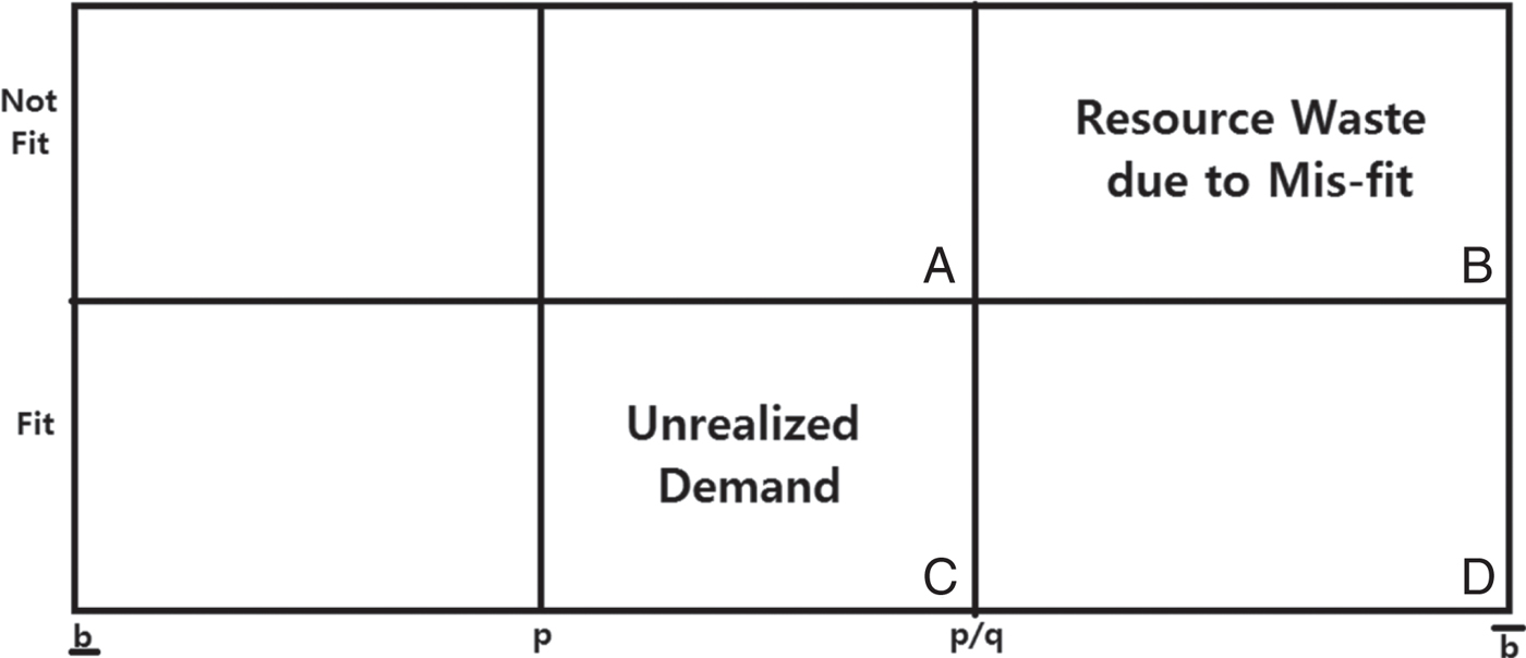
Figure 1. Sources of inefficiency due to fit-risk
Let welfare be defined as the net surplus generated by the technology, which is the net benefits from the technology and can be measured as the sum of the private value to the consumers and social value less the cost of the technology. Recall that the benefits will be reaped by only q proportion of the population, whereas the costs are incurred by the entire mass of population acquiring the technology. Let welfare be denoted by sw i , i=0, 1, where a subscript 0 denotes the value of the variables in the presence of fit-risk, and a subscript 1 denotes the value of the variables in the absence of fit-risk. Given probability of fit q, social value v, and per unit cost of technology c, welfare in the presence of fit-risk is given by
 $$sw_{0} \lpar {p,q} \rpar =\int_{{p}\over{q}}^{\bar{b}} \lpar {q\lpar {b+v} \rpar -c} \rpar f(b)db.$$
Similarly, potential welfare in the absence of fit-risk is given by
 $$sw_{1} \lpar {p,q} \rpar =q\int_{p}^{\bar{b}} \lpar {b+v-c} \rpar f(b)db.$$
The loss in welfare due to fit-risk is given by
 $$\eqalign{& sw_{1} \lpar {p,q} \rpar -sw_{0} \lpar {p,q} \rpar \cr & \quad=\int_{p}^{\bar{b}} q\lpar {b+v-c} \rpar f(b)db-\int_{{p}\over{q}}^{\bar{b}} \lpar {q\lpar {b+v} \rpar -c} \rpar f(b)db,}$$
which can be expressed as
 $$=\underbrace{\hbox{q}\int_{p}^{{p}\over{{\rm q}}} \lpar {b+v-c} \rpar f(b)db}_{lossfromURD} +\underbrace{\lpar {1-\hbox{q}} \rpar \int_{{p}\over{{\rm q}}}^{\bar{b}} cf(b)db}_{lossfromRW}.$$
Observe that the above two terms represent the value of the loss associated with two distortions in demand caused by fit-risk, and thus correspond to the two terms given in equation (6).
In proposition 1, we examine how changes in price and likelihood of fit affect the two sources of distortion in demand, namely, unrealized demand and waste.
Proposition 1
For given p, q, and 0<q<1:
-
(i) Waste is decreasing in p and non-monotonic in q;
-
(ii) Unrealized demand is increasing in p if
 $f(p/q)\ge q f(p)$
;
$f(p/q)\ge q f(p)$
; -
(iii) A sufficient condition for the unrealized demand to be decreasing in q is that the elasticity of distribution function (EDF) > 1, where
$EDF \equiv {bf(b)\over F(b)}$
; -
(iv) If the benefit b is distributed uniformly over
$\left[\underline{b},\bar{b}\right]$
, the unrealized demand is decreasing in q and increasing in p for
${{\hbox{p}}\over{\bar{b}}}<q<1.$


Parts (i) and (ii) together show that a subsidy policy (via decreasing price) may reduce unrealized demand, but would increase waste. At lower prices consumers would be more inclined to buy the technology. But since
 $\lpar {1-q}\rpar $
proportion of the acquired technology will not be utilized due to misfit, waste would also be higher as more of it is acquired, and would lead to lower welfare. Thus it is important to understand the optimal level of subsidy in the presence of fit-risk. The non-monotonic relationship between resource waste and q is another interesting result. It might seem intuitive that waste should be monotonically decreasing in q as better fit should imply less waste of resources. With an increase in q, however, there are two opposite forces affecting resource waste. One, as q increases the technology fits a greater proportion of the population reducing the waste due to misfit. But with an increase in q, the demand also increases, having the effect of increasing waste. The net effect of an increase in q would depend on the relative strengths of these two effects. At sufficiently low levels of fit, the demand effect dominates the fitness effect and waste is increasing in q. When q becomes sufficiently large, the fitness effect dominates the demand effect, and waste is decreasing in q.
$\lpar {1-q}\rpar $
proportion of the acquired technology will not be utilized due to misfit, waste would also be higher as more of it is acquired, and would lead to lower welfare. Thus it is important to understand the optimal level of subsidy in the presence of fit-risk. The non-monotonic relationship between resource waste and q is another interesting result. It might seem intuitive that waste should be monotonically decreasing in q as better fit should imply less waste of resources. With an increase in q, however, there are two opposite forces affecting resource waste. One, as q increases the technology fits a greater proportion of the population reducing the waste due to misfit. But with an increase in q, the demand also increases, having the effect of increasing waste. The net effect of an increase in q would depend on the relative strengths of these two effects. At sufficiently low levels of fit, the demand effect dominates the fitness effect and waste is increasing in q. When q becomes sufficiently large, the fitness effect dominates the demand effect, and waste is decreasing in q.
Part (ii) of proposition 1 further implies that the impact of price to expand unrealized adoption depends not only on the distribution of private benefit amongst the population, but also on the level of technology fit. Part (iii) indicates that if the CDF of private benefit distribution increases rapidly relative to the change in private benefit b, unrealized demand decreases as the likelihood of fit increases. This result might seem intuitive because if more people value technology (i.e., more density or higher b), they tend to acquire technology more as the likelihood of fit increases, and thus unrealized demand decreases. Part (iv) presents these results for a uniform distribution.
Figure 2 plots unrealized demand and resource waste across different fit probability, q, assuming b to be uniformly distributed over
 $\lsqb {0,1} \rsqb ,$
and assigning numerical values of 0.3 to the price of the technology p. It can be readily seen from figure 2 that at low probability of fit, the size of unrealized demand is greater than the size of resource waste. However, for a sufficiently high level of probability of fit, the size of waste dominates the size of unrealized demand. Thus for sufficiently high q, elimination of fit-risk may lead to a decrease in demand.
$\lsqb {0,1} \rsqb ,$
and assigning numerical values of 0.3 to the price of the technology p. It can be readily seen from figure 2 that at low probability of fit, the size of unrealized demand is greater than the size of resource waste. However, for a sufficiently high level of probability of fit, the size of waste dominates the size of unrealized demand. Thus for sufficiently high q, elimination of fit-risk may lead to a decrease in demand.

Figure 2. Unrealized demand (URD) and resource waste (RW)
In the next section, we discuss how the existence of fit-risk affects donors’ decision on price via providing a subsidy.
3. Optimal subsidy and project value
Recall that the technology has an externality v associated with it. Project donors may want to promote the technology beyond its market demand due to the positive externality associated with it. Thus, they consider providing a subsidy to lower the price of acquisition.
Suppose that project donors want to maximize welfare from their projects. From equation (9), given probability of fit q, social value v, and per unit cost of technology c, donors maximize the objective (welfare) function with respect to price p
 $$\matrix{{Max} \cr p} sw_{0} =\int_{{p}\over{q}}^{\bar{b}} \lpar {q\lpar {b+v} \rpar -c} \rpar f(b)db.$$
Let superscript ^ denote the optimal value of variables. Differentiating sw 0 with respect to p, and using the fundamental theorem of calculus, socially optimal price is given by
 $${\hat p_0} = c - vq,$$
implying a socially optimal subsidy
 $${\hat s_0} = vq,$$
since subsidy s=c−p. A subsidy internalizes the social value v associated with the technology, and since the technology fits to only q proportion of the population, the subsidy is accordingly adjusted to vq.
If, however, individuals knew whether the technology fit them or not, i.e., there is no fit-risk, donors’ objective function follows from equation (10):
 $$\matrix{{Max} \cr p} sw_{1} =q\int_{p}^{\bar{b}} \lpar {b+v-c} \rpar f(b)db.$$
Proceeding in the same manner as above, maximizing sw 1 with respect to p, we obtain the optimal subsidy ŝ 1 in the absence of fit-risk
 $${\hat s_1} = v.$$
The loss of welfare due to fit-risk, after implementation of an optimal subsidy, is given by
 $$\widehat{sw_{1}}-\widehat{sw}_{0} =q\int_{c-v}^{\bar{b}} \lpar {b+v-c} \rpar f(b)db-\int_{{c-vq}\over{q}}^{\bar{b}} \lpar {q\lpar {b+v} \rpar -c} \rpar f(b)db,$$
which can be expressed as
 $$=q\int_{c-v}^{{c-vq}\over{q}} \lpar {b+v-c} \rpar f(b)db+\lpar {1-q} \rpar \int_{{c-vq}\over{q}}^{\bar{b}} cf(b)db.$$
Proposition 2
-
(i) Fit-risk reduces the optimal level of subsidy;
-
(ii) A subsidy increases demand, but also increases waste associated with fit-risk;
-
(iii) A subsidy does not address welfare loss caused by fit-risk.
Part (i) of proposition 2 is intuitive. Since in the presence of fit-risk expected social value drops from v to qv, the optimal level of subsidy in the presence of fit-risk is smaller than the optimal subsidy when there is no fit-risk. If donors ignore this leakage in potential welfare they may over-subsidize. Part (ii) suggests that a subsidy policy increases quantity demanded not only through reducing unrealized demand, but also by generating waste. An increase in waste has a welfare-reducing effect. Thus, even when donors take into account fit-risk while deciding the optimal subsidy, they cannot prevent waste due to misfit. Since society bears the cost of wasted products, the overall welfare may decrease if donors do not take action to address it.
Part (iii) of proposition 2 suggests that there is a potential to increase welfare through elimination of fit-risk, which is given by (19). Donors, however, need to compare the cost of marketing efforts to eliminate fit-risk with its potential benefit. Demonstration is one such marketing tool that helps to reduce fit-risk. The next section presents gains from demonstration, and section 5 analyzes when it is optimal to undertake demonstration taking into account its costs.
Figures 3(a) and 3(b) illustrate demand and resource waste generated as a function of probability of fit q, assuming c=0.3, v=0.2, b is distributed uniformly over
 $\lsqb {\underline{b}}\enspace \bar{b}\rsqb ,$
and a subsidy as perceived optimal for the two cases – presence and absence of fit-risk. Figures 4(a) and 4(b) show the social welfare (project value) under the subsidy levels and assumptions of figure 3.
$\lsqb {\underline{b}}\enspace \bar{b}\rsqb ,$
and a subsidy as perceived optimal for the two cases – presence and absence of fit-risk. Figures 4(a) and 4(b) show the social welfare (project value) under the subsidy levels and assumptions of figure 3.

Figure 3. Demand (a) and waste (b)

Figure 4. Welfare from development projects
4. Demonstration gain function
Donors realize that the presence of fit-risk causes welfare loss. They may take measures to reduce it. It is worthwhile to correct the distortions caused by fit-risk if the cost of correction is smaller than the gain. Demonstration is a marketing tool that reduces fit-risk by enabling individuals to find out whether the technology fits them, so that they are more likely to make the right decision. The effect of demonstration may depend on duration, effort and intensity of demonstration. Demonstration is perfect when it eliminates all fit-risk and individuals get fully informed about fit. For simplicity we assume perfect demonstration in this paper.
To first focus on gains from demonstration, we ignore the cost of demonstration and also suppress social value v in this section.Footnote 8 To compare gains from demonstration to its cost, we will introduce demonstration cost and bring back social value in the next section. To understand the role of demonstration in eliminating fit-risk and comparing its effect across different levels of q, we construct the Demonstration Gain Function. Demonstration results in better allocation of technology among the targeted population via the two channels discussed before – by generating additional adopters who would not have acquired the technology due to fit-risk, and by preventing waste due to mismatch. The efficiency gains from demonstration, thus, are comprised of the net additional value generated due to increased adoption, and the value of resources that are prevented from being wasted. These gains are expressed in the demonstration gain function provided in proposition 3.
Let us also clarify that in our setup the role of demonstration is not to increase the fitness of the technology.Footnote 9 Demonstration helps reveal its suitability to the potential adopters so that they buy the technology only if it matches them individually.
Proposition 3
Assume perfect demonstration.
-
(i) The Demonstration Gain Function is given by.
(20)
$$G(q)=\left\{\matrix{\displaystyle {q\int_{p}^{p \over q} \lpar {b-c} \rpar f\lpar b \rpar db+\lpar {1-q} \rpar \int_{{p}\over{q}}^{\bar{b}} cf(b)db} & if\ {p \over \bar{b}}\le q\le 1 \cr \displaystyle {q\int_{p}^{\bar{b}} \lpar {b-c} \rpar f\lpar b \rpar db} \hfill & if\ 0\le q< {p \over \bar{b}}.}\right.$$
-
(ii) The Demonstration Gain Function is an increasing function of q for
$0\le q<{{p}\over{\bar{b}}}$
and a strictly concave function of q for
${{p}\over{\bar{b}}}\le q\le 1.$
-
(iii) G(q) is positive for 0<q<1, and
$\lim_{q\to 0} G(q)=\lim_{q\to 1} G(q)=0.$
-
(iv) G(q) has a maximu m between
${{p}\over{\bar{b}}}\le q\le 1.$


The two equations for the Demonstration Gain Function on the right-hand side of (20) for different ranges of q can be explained as follows: for
 ${{p}\over{\bar{b}}}\le q\le 1,$
the demonstration results in gains through both channels – by inducing more demand and also by preventing waste. For sufficiently low levels of
${{p}\over{\bar{b}}}\le q\le 1,$
the demonstration results in gains through both channels – by inducing more demand and also by preventing waste. For sufficiently low levels of
 $0\le q<{{p}\over{\bar{b}}}$
, the market demand in the absence of demonstration is zero. Since at zero demand there is no waste of resources, demonstration does not prevent any waste through this channel. Demonstration results in efficiency gains only by inducing positive demand from consumers for whom the technology fits.
$0\le q<{{p}\over{\bar{b}}}$
, the market demand in the absence of demonstration is zero. Since at zero demand there is no waste of resources, demonstration does not prevent any waste through this channel. Demonstration results in efficiency gains only by inducing positive demand from consumers for whom the technology fits.
Recall the non-monotonic relationship between q and waste due to differences between acquisition and usage (proposition 1, part (i)). Proposition 3 further builds on this relationship. It shows that if the technology is a complete misfit
 $\lpar {q=0} \rpar $
or a perfect fit (q=1), demonstration does not help. However, in the interior values of q, demonstration improves welfare.
$\lpar {q=0} \rpar $
or a perfect fit (q=1), demonstration does not help. However, in the interior values of q, demonstration improves welfare.
A visual presentation of a demonstration gain function appears in figure 5. In the figure, the difference between the gain from demonstration (the curve consisting of dots) and the waste due to fit-risk (the curve consisting of triangles) is due to the additional adoption (acquisition and use) because of demonstration. Notice that the gains from demonstration are higher at internal values of fit as compared to the extremes. If q approaches one, the technology fits everybody. Since there is no fit-risk, there is no additional information gain from demonstration. If q approaches zero, the technology does not fit anyone, and the market demand approaches zero as well. Again, there is no gain from demonstration if the technology does not fit the local population and is not demanded by them.

Figure 5. Demonstration gain function
5. Implementing demonstration with subsidy
In this section we resume social value v and also introduce cost of demonstration. Active donors or policy designers may consider combining both subsidy and demonstration strategies for their development projects. The donor's optimization problem can be formulated as a two-step decision problem in which the donor chooses an optimal level of demonstration in the first step, and an optimal subsidy in the second step in order to maximize welfare (project value). We further assume that demonstration is a binary variable that can take values 0 or 1, and the level of subsidy is a continuous variable. Denote D as a binary variable that takes a value of 1 if demonstration is used and 0 if demonstration is not used. Following Heiman et al., (Reference Heiman, McWilliams and Zilberman2001), we assume that the cost of demonstration E is a fixed cost.Footnote 10 For example, costs of demonstration can be thought of as sending a demonstrator to a region to explain the product and facilitate its trial amongst the population. Other examples include setting up a trial room/space for people to try the product, or having a few trial pieces of the new product called testers. In all these examples, demonstration costs are fixed. The donor's optimization problem can be termed as a discrete-continuous decision problem, where she maximizes project value, SW
 $$\max SW \lpar {D,s} \rpar =\matrix{max \hfill \cr D\in\left\{0,1\right\}} \left\{(D(\matrix{max \hfill \cr \quad s} sw_1(s)-E)),((1-D)\matrix{max \hfill \cr \quad s}sw_0(s))\right\}.$$
Using recursive induction, the donors first solve for the optimal level of subsidy under each case
 $\lpar {D=1,D=0} \rpar $
, and then the optimal D is determined by comparing net welfare gains under demonstration and no demonstration.
$\lpar {D=1,D=0} \rpar $
, and then the optimal D is determined by comparing net welfare gains under demonstration and no demonstration.
Let
 $s\lpar D \rpar ,D=0,1,$
denote optimal subsidy in the second step. Notice that the case of demonstration D=1 corresponds to a situation where fit-risk is eliminated, or absence of fit-risk, and D=0 corresponds to the presence of fit-risk. We have already solved for optimal subsidies for the two cases in section 3. From equations (15) and (17), the optimal subsidies are given by
$s\lpar D \rpar ,D=0,1,$
denote optimal subsidy in the second step. Notice that the case of demonstration D=1 corresponds to a situation where fit-risk is eliminated, or absence of fit-risk, and D=0 corresponds to the presence of fit-risk. We have already solved for optimal subsidies for the two cases in section 3. From equations (15) and (17), the optimal subsidies are given by
 $$s\lpar 1 \rpar =v $$
 $$s(0)=qv,$$
implying that optimal prices are
 $$p=\left\{\matrix{c-v, if D=1 \cr c-vq, if D=0}\right..$$
Plugging the optimal subsidies obtained in the second step into the first step of the optimization problem,
 $$SW\lpar {1,s\lpar 1 \rpar } \rpar =q\int_{c-v}^{\bar{b}} \lpar {b+v-c} \rpar f(b)db-E $$
 $$SW\lpar {0,\hbox{s}(0)} \rpar =\int_{{c-vq}\over{q}}^{\bar{b}} \lpar {q\lpar {b+v)-c} \rpar } \rpar f(b)db,$$
where
 $SW\lpar {D,s\lpar D \rpar } \rpar $
, D=0, 1 denotes net welfare in the first step. The donor would choose demonstration only if
$SW\lpar {D,s\lpar D \rpar } \rpar $
, D=0, 1 denotes net welfare in the first step. The donor would choose demonstration only if
 $SW\lpar 1,s\lpar 1\rpar \rpar \ge SW\lpar 0,s\lpar 0\rpar \rpar \!,$
otherwise no demonstration is chosen. Rearranging terms, demonstration would be chosen if
$SW\lpar 1,s\lpar 1\rpar \rpar \ge SW\lpar 0,s\lpar 0\rpar \rpar \!,$
otherwise no demonstration is chosen. Rearranging terms, demonstration would be chosen if
 $$\left\{\matrix{\displaystyle q\int_{c-v}^{c-vq \over q} \lpar {b + v - c} \rpar f(b)db + \lpar {1-q} \rpar \int_{c-vq \over q}^{\bar{b}} cf(b)db\ge E \hfill &{if} \,\tau \le q\le 1 \cr \displaystyle q\int_{c-v}^{\bar{b}} \lpar {b + v - c} \rpar f(b)db\ge E \hfill &{if} \, 0\le q \lt \tau }\right.$$
where
 $\tau \equiv {{c}\over{\bar{b}+v}}$
.
$\tau \equiv {{c}\over{\bar{b}+v}}$
.
Note that the left-hand side of the above equation is the same as G(q) defined in (20) with social value v and an appropriate subsidy level. This implies that if G(q)−E≥0, implementing demonstration with subsidy v improves the efficiency of a project and achieves higher welfare. The roots of (27) would determine the lower bound q l , and the upper bound q u , of the range of q for which demonstration would be optimal.
Proposition 4
Under perfect demonstration, social value v, and demonstration cost 0<E<Gmax, where
 $Gmax\equiv \matrix{max \cr q} G(q):$
-
(i) There exists an upper bound q u and a lower bound q l of q, such that demonstration improves welfare for
$0<q_{l} \le q\le q_{u} <1$
, -
(ii) The upper bound
$q_{u} \lpar {\hbox{lower bound\ q}_{l}}\rpar $
is decreasing (increasing) in demonstration costs E.


A visual presentation of a demonstration gain function assuming c=0.3, v=0.2, an optimal subsidy, and an arbitrary demonstration cost E=0.04 appears in figure 6. In this figure, demonstration improves welfare if q lies in the interior of two points where the demonstration gain function (dots) and the demonstration cost (dashed line) intersect, i.e., q u and q l. If the demonstration cost is sufficiently low such that the net gain from demonstration is positive, then demonstration with an optimal level of subsidy would lead to higher welfare as compared to an outcome when only subsidy is employed as a policy tool. It is also important to note that demonstration may actually reduce demand but increases efficiency by reducing waste.

Figure 6. Demonstration gain and cost
6. Extension
Thus far we have assumed demonstration cost to be constant and considered demonstration as a binary decision problem. However, demonstration may be a continuous variable and cost of demonstration may be increasing in the intensity of demonstration. Suppose cost of demonstration,
 $E\lpar .\rpar $
, has both fixed and variable components. Let
$E\lpar .\rpar $
, has both fixed and variable components. Let
 $E\lpar \delta \rpar =\bar{E}+\delta(a)$
, where α denotes share of population that is provided demonstration,
$E\lpar \delta \rpar =\bar{E}+\delta(a)$
, where α denotes share of population that is provided demonstration,
 $\bar{E}$
is fixed cost of demonstration, e.g., setting up a showroom, and
$\bar{E}$
is fixed cost of demonstration, e.g., setting up a showroom, and
 $\delta (\alpha)$
is variable cost of demonstration that is increasing and convex in the share of population that is given demonstration, i.e.,
$\delta (\alpha)$
is variable cost of demonstration that is increasing and convex in the share of population that is given demonstration, i.e.,
 ${\delta}'(\alpha) \ge 0$
,
${\delta}'(\alpha) \ge 0$
,
 ${\delta}''(\alpha) \ge 0$
.
${\delta}''(\alpha) \ge 0$
.
As in section 5, the donor's optimization problem is solved in two steps. In the first step, the donor decides whether or not to give demonstration. If, however, the donor chooses to provide demonstration in the first step, the second step involves simultaneously choosing three decision variables, namely subsidy for those who do not receive demonstration, s 0, subsidy for those who have demonstration, s 1, and the share of population that is given demonstration, α. The reason that we have two subsidy levels is that the products with and without demonstration are differentiated products and have different prices, where p 0=c−s 0, and p 1=c−s 1.Footnote 11
Let sw 0 and sw 1 denote welfare under fit-risk (i.e., no demonstration), and welfare in the absence of fit-risk (i.e., perfect demonstration), respectively. Let sw(α) denote net welfare (net of cost of demonstration) when only α proportion of the population gets demonstration, and is given by
 $$sw(\alpha)=\alpha sw_{1} +\lpar {1-\alpha}\rpar sw_{0}-\bar{E}-\delta(\alpha).$$
We solve the optimization problem using backward induction solving the second step first. From (13) and (16), the donor's second step optimization problem when donors decide to give demonstration in the first step is given by
 $$\eqalign{\matrix{{max} \cr {\alpha ,p_{0,} p_{1}}} sw(\alpha)&= \alpha \left(q\int_{p_{1} }^{\bar{b}} \lpar {b+v-c} \rpar f(b)db\right) +\lpar {1-\alpha }\rpar\cr & \quad \times \left({\int_{{p_{0}}\over{q}}^{\bar{b}} \lpar q\lpar {b+v} \rpar -c\rpar f(b)db} \right)-\bar{E}-\delta (\alpha).}$$
Assuming interior solution, the firstorder conditions are given by
 $$\left({q\int_{p_{1} }^{\bar{b}} \lpar {b+v-c} \rpar f(b)db} \right)-\left({\int_{{p_{0} }\over{q}}^{\bar{b}} \lpar {q\lpar {b+v} \rpar -c} \rpar f\lpar b\rpar db} \right)={\delta }'(\alpha)$$
 $$-\alpha q\lpar {p_{1} +v-c} \rpar f\lpar {p_{1} } \rpar =0$$
 $$-\lpar {1-\alpha } \rpar \left({q\left({{p_{0} }\over{q}}+{v} \right)-c} \right)f\left({{p_{0} }\over{q}} \right){1\over q}=0.$$
First-order condition (30) implies that if there is increasing marginal cost of demonstration, it is optimal to demonstrate as long as marginal benefit from implementing the demonstration is greater than its marginal cost. The marginal benefit is simply the difference between the welfare in the absence of fit-risk and the welfare in the presence of fit-risk. From (31) and (32), the optimum prices for those who have demonstration and those without demonstration equate the marginal benefit of each subsidy with that of its cost. It is evident that in the interior solution
 $\hat{p}_{1}=c-v, \hat{p}_{0}=-vq$
, implying that
$\hat{p}_{1}=c-v, \hat{p}_{0}=-vq$
, implying that
 $\widehat{s_{1}}=v, \hat{s}_{0} = v q$
where superscript ^ denotes the optimal value of variables.
$\widehat{s_{1}}=v, \hat{s}_{0} = v q$
where superscript ^ denotes the optimal value of variables.
If donors decide not to give demonstration in the first step, then they choose optimal s in the second step and the analysis is the same as that given in section 5. From (23), s(0)=qv. In the first step, the donor decides whether or not to give demonstration (i.e.,
 $D=1\ \hbox{or}\ D=0)$
.
$D=1\ \hbox{or}\ D=0)$
.
 $$\max SW=\mathop{max}\limits_{D\in \{{0,1}\}} \lcub (D\big(sw(\hat{\alpha},\hat{s}_1,\hat{s}_0)\big), ((1-D)sw_0(s(0))\rcub $$
where SW denotes net welfare in the first step. Thus donors give demonstration only if the net welfare with demonstration when an optimal share of population is provided demonstration is larger than the welfare without demonstration. The above analysis may justify providing limited promotion for a new technology in development projects. Project donors and managers may determine the optimal level of promotion campaign, and offer better promotion (i.e., demonstration with higher subsidy) for a limited time only.
We can think of many interesting outcomes of this generalization. If targeted populations are scattered across different villages and demonstration costs increase per village covered then a project manager may consider partial coverage of villages. In this case, the number of villages selected is such that the expected gain from demonstration is greater than the cost of demonstration.
An alternative extension and formulation of the model could be to the case where the project manager knows private benefit b i of each individual. In this formulation, the optimal policy is to target demonstration to the individuals whose marginal benefit from demonstration equals the marginal cost of demonstration. This may have implications for equity and result in unequal distribution of benefits from new technologies, as individuals with higher private benefit would be selected for demonstration. Zilberman et al., (Reference Zilberman, Lipper and McCarthy2008) explores program adoption decision for payment for environmental services (PES) and discusses different impacts of PES on welfare across different factor agents.
7. Conclusion
This paper attempts to introduce fit-risk in the development context and investigates potential mistakes that donors can make by ignoring it. Our analysis finds that in the presence of fit-risk there is always unrealized demand and waste. Ignoring fit-risk results in miscalculation of project values. A subsidy policy may increase demand but may also increase waste. Marketing tools such as demonstration can be used to reduce fit-risk and improve the precision of technology provision in development projects. It increases efficiency by providing a better match between individuals and the product; it does not, however, necessarily increase market demand. When demonstration is costly, demonstration use may be inefficient if the probability of fit among the targeted population is either very low or very high. The policy implications of our results are that, while promoting new technologies, development donors, governments and NGOs should take into account fit-risk and take measures to reduce it. Demonstration should be introduced when it is not too expensive. Governments may invest in reducing the cost of demonstration by providing required infrastructure, which will save precious resources.
The paper has used a simple stylized model to emphasize the role of fit-risk and demonstration in technology adoption. We analyzed optimal levels of subsidy and the decision on implementing demonstration given the predetermined level of technology fit and distribution of private benefit from the technology adoption. Future research may estimate fit-risk of different technologies and to what extent the nature of the technology affects its fit-risk.
We also assumed that demonstration is perfect, i.e., it eliminates all uncertainty. Sometimes, the effect of demonstration may not be immediate since people take time to realize the suitability of the new technology, e.g., computer languages or software. It is also possible that even after demonstration, people are unsure of the suitability of the product. Under imperfect demonstration, demonstration will still reduce fit-risk but gains from demonstration may be lower. In such cases, combining demonstration with another marketing tool such as MBG may be useful. Future research can expand the analysis to include alternative demonstration strategies that vary in their costs and effectiveness and other marketing tools that have not been emphasized in the development context.
The conceptual framework presented here, however, contributes to the use of evaluation, design and marketing strategies in development practice and technology diffusion. We hope that recognition of fit-risk opens a new avenue for empirical research. Quantifying the effectiveness of marketing mechanisms that aim to reduce fit-risk in different development project settings is an important empirical challenge for development donors, governments and NPOs. Future research should also assess the benefits and costs of demonstration and other mechanisms to address fit-risk, and utilize it in the introduction of resource-conserving, environmentally friendly technologies. Experiments can be conducted to design demonstration strategies.
Appendix
Proof of proposition 1
-
(i)
${\partial RW\over\partial q}=-\int_{{p}\over{q}}^{\bar{b}} f(b)db+\lpar {1-q} \rpar {p\over {q^{2}}}f\lpar {p\over q} \rpar$
It can be seen that
$\lim_{q\to 1} {\partial RW \over \partial q}= -\displaystyle \int_{p}^{\bar{b}} f(b)db<0$
;
$\lim_{q\to {{\rm p}\over{\bar{b}}}} {{\partial RW}\over{\partial q}}=\left(1-{{\hbox{p}}\over{\bar{b}}}\right)f\left({{\hbox{p}}\over{\bar{b}}}\right)\left({\bar{b}^{2}}\over{p}\right)>0$
. Since RW is a continuous function on
${p\over{\bar{b}}} \lt q \lt 1$
, it is negative in the neighborhood of q=1, and positive in the neighbourbood of
$q={{\hbox{p}}\over{\bar{b}}}.$
-
(ii)
${dURD \over dp}=f\lpar {{p}\over{q}} \rpar -qf\lpar p\rpar \ge \lpar <\rpar 0$
if
$f\lpar {{p}\over{q}} \rpar \ge \lpar <\rpar qf\lpar p\rpar $
. -
(iii)
${{dURD}\over{dq}}=F\lpar {{p}\over{q}} \rpar -{{\partial F\lpar {{p}\over{q}} \rpar }\over{\partial \lpar {{p}\over{q}} \rpar }}.{{p}\over{q}}-F\lpar p\rpar $
${{dURD}\over{dq}}\lt 0 \,{if}\, F\lpar {p/q}\rpar -{{\lpar {p/q} \rpar \partial F\lpar {p/q} \rpar }\over{\partial \lpar {p/q} \rpar }}\lt F\lpar p\rpar $
A sufficient condition for the above inequality to hold is
${{bf\lpar b\rpar }\over{F(b)}}\gt 1$
for all b. -
(iv) Let b be distributed uniformly over
$[\underline{b}\,\, \bar{b}]$
, for
$0<q\le {{\hbox{p}}\over{\bar{b}}}$
, quantity demand is zero under fit-risk. Therefore unrealized demand can be expressed as
For
$$\eqalign{& URD\lpar {p,q}\rpar =q\int_{p}^{\bar{b}} f(b)db={q\over\bar{b}} (\bar{b}-p)\cr & \quad \quad {\partial URD \over \partial q}={\lpar {\bar{b}}- p\rpar \over{\bar{b}-\underline{b}}}>0, {\partial URD\over\partial p}={{-1}\over{\bar{b}-\underline{b}}}< 0.}$$
${{p}\over{\bar{b}}}<q<1$
, quantity demand is positive and unrealized demand is
$$\eqalign{& URD\lpar {p,q}\rpar =q\int_{p}^{{\rm p}\over{q}} f(b)db={q\over\bar{b}-\underline{b}}\left({{p}\over{q}}-p\right) \cr & \quad {\partial URD \over {\partial q}} =-{{p}\over(\overline{b}-\underline{b})}< 0, {\partial URD \over {\partial p}}={1\over(\overline{b} -\underline{b})}\lpar 1-q\rpar >0.}$$


Derivation of (19)
Loss in welfare is given by the difference between project values in the absence and presence of fit-risk (after incorporating optimal subsidies) and can be expressed as
 $$\eqalign{\widehat{sw_{1}}-\widehat{sw}_{0} &=q\int_{c-v}^{\bar{b}} \lpar {b+v-c}\rpar f(b)db-\int_{{{\rm c}-{\rm vq}}\over{{\rm q}}}^{\bar{b}} \lsqb {q\lpar {\hbox{b}+\hbox{v}} \rpar -\hbox{c}} \rsqb \hbox{f}\lpar {\hbox{b}} \rpar \hbox{db} \cr & \quad=q\int_{c-v}^{{{\rm c}-{\rm vq}}\over{{\rm q}}} \lpar {b+v} \rpar f(b)db-q\int_{c-v}^{\bar{b}} cf(b)db+\int_{{{\rm c}-{\rm vq}}\over{{\rm q}}}^{\bar{b}} c\hbox{f}\lpar {\hbox{b}}\rpar \hbox{db} \cr & \quad=q\int_{c-v}^{{{\rm c}-{\rm vq}}\over{{\rm q}}}\lpar {b+v} \rpar f(b)db-q\int_{c-v}^{{{\rm c}-{\rm vq}}\over{{\rm q}}} cf(b)db\cr & \quad\quad +\lpar {1-q}\rpar \int_{{{\rm c}-{\rm vq}}\over{{\rm q}}}^{\bar{b}} c\hbox{f}\lpar {\hbox{b}} \rpar \hbox{db} \cr & \quad=q\int_{c-v}^{{{\rm c}-{\rm vq}}\over{{\rm q}}} \lpar {b+v-c} \rpar f(b)db+\lpar {1-q}\rpar \int_{{{\rm c}-{\rm vq}}\over{{\rm q}}}^{\bar{b}} c\hbox{f}\lpar {\hbox{b}} \rpar \hbox{db}>0\cr & \quad\quad \hbox{for}\ 0<q< 1.}$$
This would be gained from demonstration.
Proof of proposition 2:
-
(i) Follows directly from equations (15) and (17);
$\widehat{s_{0}}=vq<\hat{s}_{1} = v$
for 0<q<1. -
(ii) Substituting p=c−s into the demand Q in equation (2), we have
$$\eqalign{&\hbox{Q}\lpar {\hbox{s},\hbox{q}} \rpar =\int_{{{\rm c}-{\rm s}}\over{q}}^{\bar{b}} f(b)db \quad \cr & {{\partial Q}\over{\partial s}}={{1}\over{q}}f\left({{c-s}\over{q}} \right)>0\ \hbox{for}\ 0<q< 1.}$$
Substituting p=c−s into the RW in equation (8), we have
$$\eqalign{& RW\lpar {s,q}\rpar =\lpar {1-q}\rpar \int_{{{\rm c}-{\rm s}}\over{q}}^{\bar{b}} f(b)db \quad \cr & {\partial \hbox{RW}\over {\partial \hbox{s}}}={(1-\hbox{q}\rpar \over{q}}{f} \left(\hbox{c}-\hbox{s}\over q \right)\gt 0 \quad \hbox{for} {{c-s}\over{F^{-1}}(1)} \lt q \lt 1.}$$
-
(iii) From the proof of equation (19), the social welfare loss due to fit-risk is positive for 0<q<1, even if the optimal level of subsidy is implemented.


Proof of proposition 3
We know that
 $q={{p}\over{\bar{b}}}$
is a minimum level of fit required for the market demand to be positive. For the range of
$q={{p}\over{\bar{b}}}$
is a minimum level of fit required for the market demand to be positive. For the range of
 ${{\hbox{p}}\over{\bar{b}}}\le q\le 1$
, the gain via additional demand is
${{\hbox{p}}\over{\bar{b}}}\le q\le 1$
, the gain via additional demand is
 $q\int_{p}^{{{p}\over{q}}} \lpar {b-c}\rpar f\lpar b\rpar db$
and the gain from preventing waste is
$q\int_{p}^{{{p}\over{q}}} \lpar {b-c}\rpar f\lpar b\rpar db$
and the gain from preventing waste is
 $\lpar {1-q} \rpar \int_{{{p}\over{q}}}^{\bar{b}} cf(b)db.$
For
$\lpar {1-q} \rpar \int_{{{p}\over{q}}}^{\bar{b}} cf(b)db.$
For
 $0\le q<{{p}\over{\bar{b}}}$
, the gain from preventing waste is zero since there was no demand before demonstration, and the upper bound of the private benefit is
$0\le q<{{p}\over{\bar{b}}}$
, the gain from preventing waste is zero since there was no demand before demonstration, and the upper bound of the private benefit is
 $\bar{b}$
. Therefore, the demonstration gain function for
$\bar{b}$
. Therefore, the demonstration gain function for
 $0\le \hbox{q}<{{\hbox{p}}\over{\bar{b}}}$
becomes
$0\le \hbox{q}<{{\hbox{p}}\over{\bar{b}}}$
becomes
 $q\int_{p}^{\bar{b}} \lpar {b-c} \rpar f(b)db$
. Since the demonstration gain function is defined as the sum of gain from additional demand and gain from preventing waste, the expression for the demonstration gain function follows.
$q\int_{p}^{\bar{b}} \lpar {b-c} \rpar f(b)db$
. Since the demonstration gain function is defined as the sum of gain from additional demand and gain from preventing waste, the expression for the demonstration gain function follows.
-
(i) Let G1(q) be G(q) for
${{\hbox{p}}\over{\bar{b}}}\le \hbox{q}\le 1$
and G2(q) be G(q) for
$0\le \hbox{q}<{{\hbox{p}}\over{\bar{b}}}$
in equation (21). G1(q) is the sum of two continuous and twice differentiable functions, so it is also continuous and twice differentiable.
$$\eqalign{{\partial G1(q)\over{\partial q}}& = \int_{p}^{{p}\over{q}} \lpar {b-c} \rpar f(b)db+q\left({{p}\over{q}}-c \right)f\left({{p}\over{q}} \right)\left({-}{{p}\over{q^{2}}} \right)\cr & \quad-\int_{{p}\over{q}}^{\bar{b}} cf(b)db+\lpar {1-q} \rpar \left({{p}\over{q^{2}}} \right)cf\left({{p}\over{q}} \right)\cr & =\int_{p}^{{p}\over{q}}\! \lpar {b-c} \rpar f(b)db-\int_{{p}\over{q}}^{\bar{b}}\! cf(b)db-q\left(\!{{p}\over{q}}-{c}\!\right)f\left(\!{{p}\over{q}}\!\right)\left(\!{{p}\over{q^{2}}}\!\right)\cr & \quad+\lpar {1-q} \rpar \left({{p}\over{q^{2}}} \right)cf\left({{p}\over{q}} \right)\quad\cr & =\int_{p}^{{p}\over{q}} bf(b)db-\int_{p}^{\bar{b}} cf(b)db-\left({{p}\over{q^{2}}} \right)f\left({{p}\over{q}} \right)\lpar {p-c} \rpar \cr {\partial G1^{2}(q)\over{\partial q^{2}}}&= -\left({{p^{2}}\over{q^{3}}} \right)f\left({{p}\over{q}} \right)-\lpar {c-p} \rpar \left({{p}\over{q^{3}}} \right)f\left({{p}\over{q}} \right)\left({{2}+{p\over{q}}}\right)< 0.}$$
This is because the first term is always negative, and the second term is non-positive for p≤c. In our setting, price is either equal to (in the absence of subsidies) or less than unit cost (in the presence of subsidies). Thus G1(q) is a strictly concave function on
${{\hbox{p}}\over{\bar{b}}}\le \hbox{q}\le 1$
. For
$0\le q<{{\hbox{p}}\over{\bar{b}}}$
, G2(q) is also continuous and differentiable.
$${{\partial \hbox{G}2}\over{\partial \hbox{q}}}=\int_{p}^{\bar{b}} \lpar {b-c} \rpar f(b)db>0.$$
Therefore, G2(q) is increasing on
$0\le q<{{\hbox{p}}\over{\bar{b}}}$
. -
(ii) Follows from proposition 1 (ii) and the definition of the Demonstration Gain Function. If we plug q=0 and 1 into G(q), we know
$\lim_{q\to 0} G(q)=G(0)=G\lpar 1 \rpar =\lim_{q\to 1} G(q)=0.$
-
(iii) G1(q) is bounded and strictly concave, thus it has an interior unique maximum. Let
$\tilde{q}\equiv argmax \, \, G1(q)$
. We now show that G1(q) and G2(q) are continuous at β.
$\lim_{{\rm q}\to \beta } \hbox{G}1\lpar {\hbox{q}} \rpar =\beta \int_{p}^{\bar{b}} \lpar {b-c} \rpar f(b)db=\lim_{q\to \beta} \hbox{G}2(q)$
, thus G1(q) and G2(q) are continuous at β. Since G2(q) is positive and increasing in q, G2(q) has a maximum value at the bound of β. Thus G(q) has a unique maximum at
$\tilde{q}$
, where
$\beta \le \tilde{q}\leq <xref ref-type="disp-formula" rid="eqn1">1</xref>$
. Define
$Gmax\equiv G(\tilde{q})$
.


Proof of proposition 4
The steps of the proof are clear from figure 6.
-
(i) Define net gains from demonstration as
$H(q)\equiv G\lpar q \rpar -E.$
For
$E=0,H(q)>0\ forall\ 0<q<1.$
$\hbox{For}\ E>Gmax\equiv G(\tilde{q}),H(q)<0$
for all q. That is, for sufficiently high cost of demonstration, net gains from demonstration are negative.From proposition 3, we know that G(q) is unimodal, and intersects the x-axis at 0 and 1. Since E is constant, H(q) is also unimodal. For
$0<E<Gmax,H(q)$
intersects the x-axis at q
L
and q
U
, where q
L
and q
U
are in the interiors of 0,1. Demonstration results in positive net gains for
$q_{L} \le q\le q_{U}.$
-
(ii) From (i), we know that
$\hbox{G}\lpar {q_{l}}\rpar =E$
for
$0\le q_{l} <\tilde{q}$
. Since G(q) is a non-decreasing function in
$0\le q_{l} <\tilde{q}$
,
$q_{l}^{\prime}\equiv G^{-1}\lpar \bar{E}\rpar \geq G^{-1} (E)\equiv q_{l}$
if E′≥E. Similarly, for
$\tilde{q}\le q \le 1$
, G(q) is non-increasing, so
$q_{u}^{\prime} \equiv G^{-1}(E')\le G^{-1}(E) \equiv q_{u}$
if E′≥E.


Extension to (29): the optimization problem under uniform subsidy
 $$\eqalign{\matrix{max \cr \alpha, p} sw(\alpha)&=\alpha \left({q\int_{p}^{\bar{b}} \lpar {b+v-c} \rpar f(b)db} \right)\cr & \quad +\lpar 1-\alpha \rpar \left(\int_{p \over {q}}^{\bar{b}} [q(b+v) -c] f(b)db \right)-\bar{E}-\delta(\alpha)}$$
The first-order conditions for interior solution are given by
 $$\eqalign{&\left({q\int_{p}^{\bar{b}} \lpar {b+v-c} \rpar f(b)db} \right)-\left(\int_{{p}\over{q}}^{\bar{b}} \lsqb {q\lpar {b+v} \rpar -c} \rsqb f(b)db\right)={\delta}'(\alpha)\cr & \quad -\alpha q\lpar {p+v-c} \rpar f\lpar p \rpar -\lpar {1-\alpha}\rpar \left({q\left({p\over{q}}+{v} \right)-c} \right)f\left({{p}\over{q}} \right){{1}\over{q}}=0.}$$
It is evident that in the interior solution
 $c-v\le p\le c-qv$
, implying that v≥s≥qv.
$c-v\le p\le c-qv$
, implying that v≥s≥qv.


