


1. Introduction
Triboelectric charging plays a role in a wide range of contexts, from the static electricity generated when removing synthetic garments to handling of industrial powders. In nature, particles triboelectrically charge during volcanic eruptions (James, Lane & Gilbert Reference James, Lane and Gilbert2000; Mather & Harrison Reference Mather and Harrison2006), dust devils and sandstorms (Stow Reference Stow1969). Their charging directly influences particle dynamics and leads to measurable environmental consequences. For instance, triboelectric effects enable volcanic ash to ascend into the ionosphere, impacting Earth’s climate systems (Genge Reference Genge2018).
Amid industrial operations, particles electrify particularly during pneumatic conveying (Klinzing Reference Klinzing2018). To date the control of powder electrification has been carried out empirically (Nomura, Satoh & Masuda Reference Nomura, Satoh and Masuda2003) and even basic concepts are still being debated (Wei & Gu Reference Wei and Gu2015). As a result, hazardous spark discharges occur that are a source of fatal dust explosions, loss of lives and economic damage (Glor Reference Glor2003; Ohsawa Reference Ohsawa2011).
Past efforts to control powder charging primarily focused on the material properties of the particles and the piping system. However, the scientific advances in recent years thanks to the development of new highlysensitive measurement apparatus and detailed theoretical models (an extensive review is provided, for example, by Lacks & Troy Shinbrot (Reference Lacks and Troy2019)) indicate that a conclusive understanding of triboelectricity cannot be achieved in the near future. Matsuyama et al. (Reference Matsuyama, Ogu, Yamamoto, Marijnissen and Scarlett2003) demonstrated that even under identical impact conditions, the charge transfer between a particle and a target during contact is not reproducible. This observation is not surprising considering that the contact potential of a surface is far from being constant but instead is a temporally varying mosaic of oppositely charged regions of nanoscopic dimensions (Baytekin et al. Reference Baytekin, Patashinski, Branicki, Baytekin, Soh and Grzybowski2011). Similarly astonishing is the occurrence of bipolar charge in powders (Zhao et al. Reference Zhao, Castle, Inculet and Bailey2003; Bilici et al. Reference Bilici, Toth, Sankaran and Lacks2014). Also, it was recently demonstrated that triboelectric charging is time-dependent, irrespective of the precise charge carrier or mechanism. Moreover, shaker experiments revealed that competing processes act over multiple timescales in non-equilibrium (Shinbrot et al. Reference Shinbrot, Ferdowsi, Sundaresan and Araujo2018; Yin & Nysten Reference Yin and Nysten2018; Yin, Vanderheyden & Nysten Reference Yin, Vanderheyden and Nysten2018). This and the above-discussed findings imply that the outcome of a contact charging event may be inherently unstable, and non-reproducible. Moreover, the complexity of the underlying physics prohibits the formulation of a generally valid theoretical model. For this reason, the most common measure aiming to control particle charging, namely the manipulation of particle surfaces, has so far been of limited success.
However, there is evidence that processes acting on the macroscopic powder level may be decisive for the charging rate of particle-laden flows. Empirical analysis of powder charging during pneumatic conveying using Faraday cages revealed global trends, e.g. the relation between the flow velocity, solid mass loading or particle material and the total powder charge (Watano Reference Watano2006; Ndama, Guigon & Saleh Reference Ndama, Guigon and Saleh2011; Schwindt et al. Reference Schwindt, von Pidoll, Markus, Klausmeyer, Papalexandris and Grosshans2017; Peltonen, Murtomaa & Salonen Reference Peltonen, Murtomaa and Salonen2018). The disadvantage of this method is that it is not capable of providing a detailed view of the electrification process and the mechanisms that cause these trends cannot be expected.
For this purpose, the development of predictive numerical tools seems more promising. Large-eddy simulations, where the large turbulent scales are resolved, confirmed the strong dependence of powder charging on the flow Reynolds number, the mass flow rate of the powder and the pipe diameter (Lim, Yao & Zhao Reference Lim, Yao and Zhao2012; Korevaar et al. Reference Korevaar, Padding, Van der Hoef and Kuipers2014; Grosshans & Papalexandris Reference Grosshans and Papalexandris2016). However, large-eddy simulation is not free of potential errors, especially regarding the dynamics in the near-wall regions where charge separation takes place. Direct numerical simulations (DNS) where all turbulence scales are resolved on the grid gave evidence that the charging rate of powder may be determined by the occurrence of small-scale flow mechanisms (Grosshans & Papalexandris, Reference Grosshans and Papalexandris2017a
). More specifically, in a turbulent channel flow of
 $Re_{\tau}=180$
at moderate Stokes numbers and low particle volume fractions, the electric charge builds up but cannot escape the viscous sublayer due to the turbophoretic drift. In this case, the particles close to the wall reach at some point equilibrium charge, but most particles in the bulk remain uncharged. The complete flow can only charge if either the Stokes number or the particle number density is increased, thus giving rise to particle-bound charge transport or interparticle charge diffusion, respectively.
$Re_{\tau}=180$
at moderate Stokes numbers and low particle volume fractions, the electric charge builds up but cannot escape the viscous sublayer due to the turbophoretic drift. In this case, the particles close to the wall reach at some point equilibrium charge, but most particles in the bulk remain uncharged. The complete flow can only charge if either the Stokes number or the particle number density is increased, thus giving rise to particle-bound charge transport or interparticle charge diffusion, respectively.
In addition, flow patterns influence powder charging. For example, wall-bounded turbulence was found to suppress bipolar particle charging (Jantač & Grosshans Reference Jantač and Grosshans2024). Moreover, turbulence causes mid-sized particles to accumulate the most negative charge and not the smallest ones, as previously assumed.
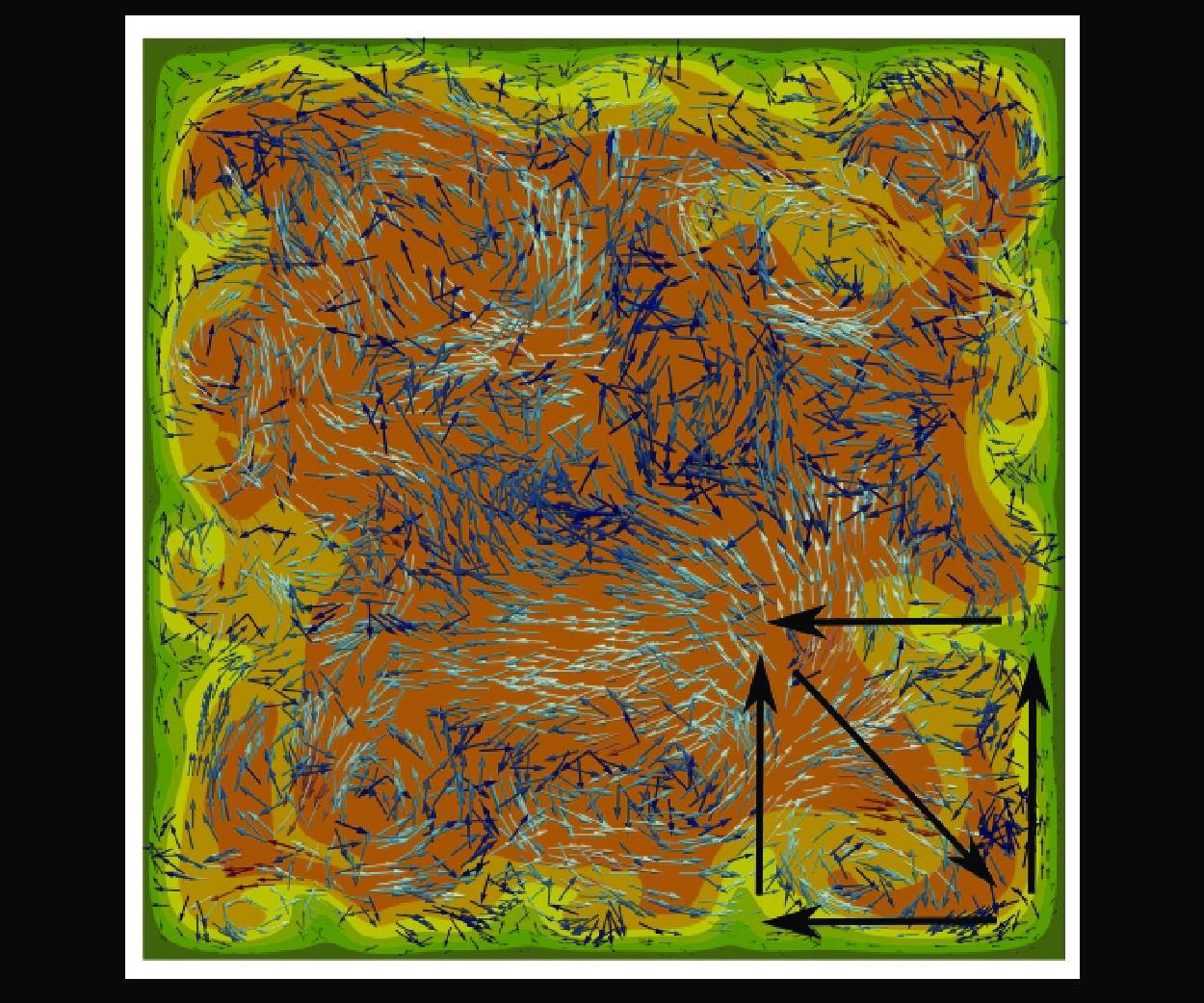
Channel flows, with their predominantly one-dimensional nature, are mainly affected by proximity to the walls. Conversely, duct flows lack a uniform direction, resulting in cross-sectional secondary flow structures, as illustrated in figure 1(b). Although weaker, these secondary flows significantly impact particle behaviour by altering fluid velocity gradients. The interaction of cross vortices accelerates particles towards the walls, increasing their collision frequency. This secondary flow drives particles from the corners along the walls towards the centre, enhancing uniform mixing within the duct. In contrast, in channels, particles at the wall are driven towards the bulk of the flow primarily through a random sequence of small-scale turbulent motions. Thus, a greater number of particles are concentrated near the wall which reduces particle-bound charge transport.

Figure 1. Normalized streamwise velocity contours and cross velocity vectors of fluid in channel flow (a) and duct flow (b) cross-sections. The lower left half of the channel and lower half of the duct are shown. Arrows represent the direction of the secondary flows. The confined area shows fluid acceleration to the corners due to coinciding vortices.
Upon charging, particles experience substantial changes in their behaviour. Measurements of the mean electric field generated by charged dust particles indicate strengths that could be comparable to gravitational forces, potentially leading to the elevation of dust in the presence of electric fields (Kok & Renno Reference Kok and Renno2008). Grosshans et al. (Reference Grosshans, Bissinger, Calero and Papalexandris2021) employed DNS to explore how electrostatic forces affect wall turbulence in a square duct with monodisperse charged particles. Their findings revealed an active suppression of the vortical motion of particles within secondary flow structures by electrostatic forces. Consequently, there was a significant increase in particle number density at the bisectors of the walls. Another study, utilizing DNS of mono- and bidisperse particles at a friction Reynolds number
 $Re_\tau =550$
in turbulent channel flow, reveals significant alterations in particle behaviour when the electrostatic Stokes number is of
$Re_\tau =550$
in turbulent channel flow, reveals significant alterations in particle behaviour when the electrostatic Stokes number is of
 $O(10^{-1})$
(Zhang, Cui & Zheng Reference Zhang, Cui and Zheng2023). These changes in the particles’ behaviours due to the charging of powder result in alterations in the fluid field. A more recent DNS study of turbulent channel flow at
$O(10^{-1})$
(Zhang, Cui & Zheng Reference Zhang, Cui and Zheng2023). These changes in the particles’ behaviours due to the charging of powder result in alterations in the fluid field. A more recent DNS study of turbulent channel flow at
 $Re_\tau =540$
involving bidisperse particles shows that interparticle electrostatic forces significantly impact turbulent characteristics. Specifically, the presence of electrostatic forces alters both the intensity and structure of turbulence. It was found that the inner-scaled mean streamwise fluid velocity decreases in charged particle flows, which suggests an increase in fluid friction velocity (Zhang et al. Reference Zhang, Cui and Zheng2024).
$Re_\tau =540$
involving bidisperse particles shows that interparticle electrostatic forces significantly impact turbulent characteristics. Specifically, the presence of electrostatic forces alters both the intensity and structure of turbulence. It was found that the inner-scaled mean streamwise fluid velocity decreases in charged particle flows, which suggests an increase in fluid friction velocity (Zhang et al. Reference Zhang, Cui and Zheng2024).
Based on these recent findings, we elaborate in this study on a new way to solve the problem, namely the possible control of the triboelectric charging of powder flows by imposing certain flow dynamics.
To this end, DNS using the tool pafiX (Grosshans Reference Grosshans2021) are performed. Therein, the flow dynamics is solved in an Eulerian framework. Each particle is tracked individually as a Lagrangian point by solving Newton’s equations of motion where fluid drag, electrostatic and collisional forces are accounted for. A full description of the solver and the numerical scheme and their validation are given in Grosshans & Papalexandris (Reference Grosshans and Papalexandris2017a ) and Grosshans et al. (Reference Grosshans, Bissinger, Calero and Papalexandris2021).
The computation of electrostatic forces between charged particles is challenging due to the limitations of existing computational methods. Coulomb’s law calculates the forces between each particle directly but becomes computationally expensive for dense particulate flows as the cost scales quadratically with the number of particles,
 $O(N^{2})$
. Gauss’s law uses charge density instead of calculating individual particle interactions, making it efficient for dense flows. However, its accuracy relies on grid resolution, which must be at least comparable to the particle size to accurately capture electrostatic interactions between nearby particles.
$O(N^{2})$
. Gauss’s law uses charge density instead of calculating individual particle interactions, making it efficient for dense flows. However, its accuracy relies on grid resolution, which must be at least comparable to the particle size to accurately capture electrostatic interactions between nearby particles.
To overcome the difficulties mentioned above, several computational techniques have been developed. One example is the fast multipole method, which reduces computational costs in pairwise calculations to
 $O(N\textrm {log}N)$
by grouping distant particles (Rokhlin Reference Rokhlin1990). The combined effects of the grouped particles are then approximated by using fast multipole expansions. This approach is often applied to molecular dynamic simulations (Board et al. Reference Board, Causey, Leathrum, Windemuth and Schulten1992; Ding, Karasawa & Goddard Reference Ding, Karasawa and Goddard1992). Recently, Ruan, Gorman & Ni (Reference Ruan, Gorman and Ni2024) used this approach in particle-laden turbulent flow simulations to study the influence of charge segregation on the dynamics of bidisperse inertial particles. Although commonly used, this approach has challenges, such as numerical instability and a high error constant (Darve Reference Darve2000). Addressing these challenges requires additional techniques that add complexity to the implementation of the approach to numerical simulations.
$O(N\textrm {log}N)$
by grouping distant particles (Rokhlin Reference Rokhlin1990). The combined effects of the grouped particles are then approximated by using fast multipole expansions. This approach is often applied to molecular dynamic simulations (Board et al. Reference Board, Causey, Leathrum, Windemuth and Schulten1992; Ding, Karasawa & Goddard Reference Ding, Karasawa and Goddard1992). Recently, Ruan, Gorman & Ni (Reference Ruan, Gorman and Ni2024) used this approach in particle-laden turbulent flow simulations to study the influence of charge segregation on the dynamics of bidisperse inertial particles. Although commonly used, this approach has challenges, such as numerical instability and a high error constant (Darve Reference Darve2000). Addressing these challenges requires additional techniques that add complexity to the implementation of the approach to numerical simulations.
Another approach, the particle–mesh method, projects the particle charges onto a grid and solves the Poisson equation to determine the electric potential. This method assumes that the electrostatic forces between nearby particles are negligible compared with the collective effect of distant particles. While this makes it computationally efficient, it causes significant errors, especially for dense systems or systems where particles cluster (Yao & Capecelatro Reference Yao and Capecelatro2018).
The particle–particle particle–mesh (P3M) method (Hockney & Eastwood Reference Hockney and Eastwood1988) builds on the particle–mesh method. It uses a computational grid to approximate long-range forces by solving the Poisson equation in Fourier space while short-range forces are calculated using Coulomb’s law. To avoid double-counting from both ranges, the long-range potential is modified with a correction term, and the computational cost scales with
 $O(N\textrm {log}N)$
. The P3M method was initially designed to predict interactions between ions in electrolytic solutions. However, it has also been applied to simulations of charged inertial particles in a Taylor–Green vortex and an isotropic turbulent flow (Yao & Capecelatro Reference Yao and Capecelatro2018). While the method is useful for monodispersed, uniform particulate flows, and homogeneous charge distributions as in ionic solutions, it faces challenges when particles are clustered or when high precision is needed, which is the case in particle-laden flows. Moreover, this method’s use of Fourier transforms limits its application to periodic boundary conditions (Grosshans & Papalexandris, Reference Grosshans and Papalexandris2017c
).
$O(N\textrm {log}N)$
. The P3M method was initially designed to predict interactions between ions in electrolytic solutions. However, it has also been applied to simulations of charged inertial particles in a Taylor–Green vortex and an isotropic turbulent flow (Yao & Capecelatro Reference Yao and Capecelatro2018). While the method is useful for monodispersed, uniform particulate flows, and homogeneous charge distributions as in ionic solutions, it faces challenges when particles are clustered or when high precision is needed, which is the case in particle-laden flows. Moreover, this method’s use of Fourier transforms limits its application to periodic boundary conditions (Grosshans & Papalexandris, Reference Grosshans and Papalexandris2017c
).
The pseudo-particle method, developed by Boutsikakis, Fede & Simonin (Reference Boutsikakis, Fede and Simonin2023), estimates the short-range interactions via the sum of particle–particle interactions using Coulomb’s law, similar to the P3Mmethod. However, it differs from the P3M approach, since long-range interactions are also approximated using Coulomb’s law, but in an approximate form through pseudo-particles. In this approach, the distant particles are grouped into clusters (pseudo-particles), and their collective influence is calculated based on Coulomb’s law. The computational efficiency of the pseudo-particle method scales as
 $O(N^{1.5})$
.
$O(N^{1.5})$
.
In this work, we used the hybrid approach proposed by Grosshans & Papalexandris (Reference Grosshans and Papalexandris2017c ). In this approach, interactions between neighbouring particles (particles in the same computational cells) are computed directly using Coulomb’s law, and superposed on the particle in question; while the collective effects of particles in other cells are approximated using Gauss’s law. This approach brings similar accuracy to direct calculation using Gauss’s law and reduces computational costs by a factor of eight. Also, it is more suitable for wall-bounded flows as compared with the P3M method.
As discussed above, there is no consensus as regards the physics of the charging of individual particles. Only a few computational fluid dynamics models are available, namely the condenser model for conductive (Fuks, Sutugin & Soo Reference Fuks, Sutugin and Soo1971; Masuda, Komatsu & Iinoya Reference Masuda, Komatsu and Iinoya1976; John, Reischl & Devor Reference John, Reischl and Devor1980) and insulating (Grosshans & Papalexandris, Reference Grosshans and Papalexandris2017b ) surfaces, and models relying on the surface state theory (Lowell & Truscott Reference Lowell and Truscott1986a ,Reference Lowell and Truscott b ; Lacks & Levandovsky Reference Lacks and Levandovsky2007; Duff & Lacks Reference Duff and Lacks2008; Konopka& Kosek Reference Konopka and Kosek2017). All these models handle only very specific situations, require tuning and are, thus, not able to generally predict particle charging.
In the current simulations, we employ a simple approach that relies upon two basic relations which are commonly observed under nearly all circumstances. First, particles gain charge upon contact with another object in their contact area. Second, with repeating contact, the charge reaches asymptotically a certain saturation value or equilibrium charge,
 $q_{\mathrm {eq}}$
. This simple model is sufficient for the purpose of this study since the conclusions drawn herein are largely independent of the precise amount of exchanged charge.
$q_{\mathrm {eq}}$
. This simple model is sufficient for the purpose of this study since the conclusions drawn herein are largely independent of the precise amount of exchanged charge.
This paper is organized as follows. Section 2 details the mathematical model and computational methods employed. Section 3 describes the numerical set-up of simulations. Section 4 presents and analyses the numerical results. Finally, § 5 offers concluding remarks.
2. Mathematical model and numerical methods
We used the tool pafiX (Grosshans Reference Grosshans2021) for conducting particle-laden flow simulations. This section provides an overview of the mathematical model and computational methods employed in pafiX.
The system’s governing equations consist of three interconnected components: (i) the Navier–Stokes equations describe the flow of the carrier gas, (ii) Gauss’s law governs the electrostatic field and (iii) Newton’s law of motion controls the movement of particles. While components (i) and (ii) are established within the Eulerian framework, the equations governing particle motion are addressed using the Lagrangian approach. The model accounts for four-way coupling between the fluid and particle phases, which means momentum exchange in both directions and interactions among individual particles are considered.
For a constant-density carrier gas flow, the Navier–Stokes equations are expressed as follows:
 \begin{equation} {\nabla } \cdot {\boldsymbol {u}}=0 , \end{equation}
 \begin{equation} \frac {\partial {{\boldsymbol {u}}}}{\partial t}+ ({\boldsymbol {u}} \cdot {\nabla }){\boldsymbol {u}}=-\frac {1}{\rho _{\text{f}}}{\nabla }P+\nu \nabla ^{2}{{\boldsymbol {u}}}+{\boldsymbol {F}}_{\text{s}} + {\boldsymbol {F}}_{\text{f}}. \end{equation}
In these equations,
 $\boldsymbol {u}$
represents the velocity vector of the fluid,
$\boldsymbol {u}$
represents the velocity vector of the fluid,
 $\rho _{\text{f}}$
denotes the fluid density,
$\rho _{\text{f}}$
denotes the fluid density,
 $P$
indicates the dynamic pressure and
$P$
indicates the dynamic pressure and
 $\nu$
represents the kinematic viscosity. Equations (2.1) and (2.2) use central difference schemes of second-order accuracy to compute spatial derivatives. The temporal derivative in (2.2) is integrated via an implicit second-order scheme using a variable time step.
$\nu$
represents the kinematic viscosity. Equations (2.1) and (2.2) use central difference schemes of second-order accuracy to compute spatial derivatives. The temporal derivative in (2.2) is integrated via an implicit second-order scheme using a variable time step.
The source term,
 ${\boldsymbol {F}}_{\text{s}}$
, accounts for momentum transfer from the particles to the fluid. It is defined as the negative sum of the fluid forces acting on the particles within the control volume. This negative sign indicates that
${\boldsymbol {F}}_{\text{s}}$
, accounts for momentum transfer from the particles to the fluid. It is defined as the negative sum of the fluid forces acting on the particles within the control volume. This negative sign indicates that
 ${\boldsymbol {F}}_{\text{s}}$
represents the feedback force from the particles, which acts in the direction opposite to the fluid forces. The source term can be expressed as
${\boldsymbol {F}}_{\text{s}}$
represents the feedback force from the particles, which acts in the direction opposite to the fluid forces. The source term can be expressed as
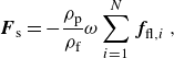 \begin{equation} {\boldsymbol {F}}_{\text{s}} = -\frac {\rho _{\text{p}}}{\rho _{\text{f}}}\omega \sum _{i=1}^{N} {\boldsymbol {f}}_{\!\text{fl},i} \,, \end{equation}
where
 $N$
is the number of particles in the same computational cell,
$N$
is the number of particles in the same computational cell,
 $\omega$
is the local particle volume fraction,
$\omega$
is the local particle volume fraction,
 $\rho _{\text{p}}$
is the particle density and
$\rho _{\text{p}}$
is the particle density and
 ${\boldsymbol {f}}_{\!\text{fl},i}$
is the acceleration due to fluid forces acting on individual particles. The fluid forces include drag and lift components and are detailed later in this section. Force
${\boldsymbol {f}}_{\!\text{fl},i}$
is the acceleration due to fluid forces acting on individual particles. The fluid forces include drag and lift components and are detailed later in this section. Force
 ${\boldsymbol {F}}_{\text{f}}$
denotes an external force applied to counterbalance the momentum dissipation of the fluid caused by wall friction.
${\boldsymbol {F}}_{\text{f}}$
denotes an external force applied to counterbalance the momentum dissipation of the fluid caused by wall friction.
The presence of charged particles generates an electric field, represented by
 $\boldsymbol {E}$
, which is related to the electric potential
$\boldsymbol {E}$
, which is related to the electric potential
 $\varphi _{\text{el}}$
through the gradient as
$\varphi _{\text{el}}$
through the gradient as
 \begin{equation} {\boldsymbol {E}} = -\nabla \varphi _{\text{el}}. \end{equation}
This electric potential
 $\varphi _{\text{el}}$
is then determined using Gauss’ law, which is
$\varphi _{\text{el}}$
is then determined using Gauss’ law, which is
 \begin{equation} \nabla ^2 \varphi _{\text{el}} = -\frac {\rho _{\text{el}}}{\varepsilon }. \end{equation}
In this equation,
 $\rho _{\text{el}}$
represents the electric charge density and
$\rho _{\text{el}}$
represents the electric charge density and
 $\varepsilon$
is the permittivity of the fluid. If no external electric field is present, the electric charge density results directly from the positions of the individual particles and their charge. The electric permittivity (
$\varepsilon$
is the permittivity of the fluid. If no external electric field is present, the electric charge density results directly from the positions of the individual particles and their charge. The electric permittivity (
 $\varepsilon$
) of a solid–gas mixture is approximated using the value of free-space permittivity (
$\varepsilon$
) of a solid–gas mixture is approximated using the value of free-space permittivity (
 $8.85 \times 10^{-12}\,\rm F\, m^-{^1}$
) due to the negligible solid volume fraction, as suggested by previous studies (Rivas & Iglesias Reference Rivas and Iglesias2007; Rokkam, Fox & Muhle Reference Rokkam, Fox and Muhle2010). Second-order central difference discretization is applied to the left-hand side of (2.5).
$8.85 \times 10^{-12}\,\rm F\, m^-{^1}$
) due to the negligible solid volume fraction, as suggested by previous studies (Rivas & Iglesias Reference Rivas and Iglesias2007; Rokkam, Fox & Muhle Reference Rokkam, Fox and Muhle2010). Second-order central difference discretization is applied to the left-hand side of (2.5).
Our simulations assume rigid, spherical particles with uniform density. These particles are smaller than the computational grid cells, allowing us to track them individually using a point-mass approach within the Lagrangian framework. Newton’s second law of motion then governs the acceleration of each particle:
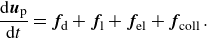 \begin{equation} \frac {\text{d} {{\boldsymbol {u}}}_{\text{p}}}{\text{d} t} = {\boldsymbol {f}}_{\!\text{d}} + {\boldsymbol {f}}_{\!\text{l}} + {\boldsymbol {f}}_{\!\text{el}} + {\boldsymbol {f}}_{\!\text{coll}}\,. \end{equation}
Here
 ${\boldsymbol {u}}_{\text{p}}$
is the particle velocity,
${\boldsymbol {u}}_{\text{p}}$
is the particle velocity,
 $\,{\boldsymbol {f}}_{\!\text{d}}$
is the aerodynamic drag,
$\,{\boldsymbol {f}}_{\!\text{d}}$
is the aerodynamic drag,
 $\,{\boldsymbol {f}}_{\!\text{l}}$
is the acceleration due to lift force,
$\,{\boldsymbol {f}}_{\!\text{l}}$
is the acceleration due to lift force,
 $\,{\boldsymbol {f}}_{\!\text{el}}$
is the particle acceleration due to the electric field and
$\,{\boldsymbol {f}}_{\!\text{el}}$
is the particle acceleration due to the electric field and
 $\,{\boldsymbol {f}}_{\!\text{coll}}$
is the collisional acceleration. The particle trajectories are solved by a second-order Crank–Nicolson scheme.
$\,{\boldsymbol {f}}_{\!\text{coll}}$
is the collisional acceleration. The particle trajectories are solved by a second-order Crank–Nicolson scheme.
The aerodynamic acceleration is given as
 \begin{equation} {\boldsymbol {f}}_{\!\text{d}}=-\frac {3\rho _{\text{f}}}{8\rho _{\text{p}} r_{\text{p}}}C_{\text{d}}\left | {\boldsymbol {u}}_{\text{rel}} \right |{\boldsymbol {u}}_{\text{rel}}\,, \end{equation}
where
 ${\boldsymbol {u}}_{\text{rel}}$
is the relative velocity between the particle and the fluid and
${\boldsymbol {u}}_{\text{rel}}$
is the relative velocity between the particle and the fluid and
 $r_{\text{p}}$
is the radius of particles. Therein the drag coefficient is based on Putnam’s correlation:
$r_{\text{p}}$
is the radius of particles. Therein the drag coefficient is based on Putnam’s correlation:
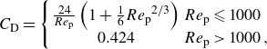 \begin{equation} C_{\text{D}} = \left \{ \begin{array}{cl} \frac {24}{Re_{\text{p}}} \left ( 1 + \frac {1}{6} {Re_{\text{p}}}^{2/3} \right ) & {Re_{\text{p}}} \leqslant 1000 \\ 0.424 & {Re_{\text{p}}} \gt 1000 \, , \end{array} \right . \end{equation}
where
 $Re_{\text{p}}$
is the particle Reynolds number,
$Re_{\text{p}}$
is the particle Reynolds number,
 $\left | {\boldsymbol {u}}_{\text{rel}} \right | d_{\text{p}}/\nu$
.
$\left | {\boldsymbol {u}}_{\text{rel}} \right | d_{\text{p}}/\nu$
.
The acceleration due to lift force according to Saffman (Reference Saffman1965) adjusted by Mei (Reference Mei1992) reads
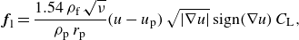 \begin{equation} {\boldsymbol {f}}_{\!\text{l}} = \frac {1.54\, \rho _{\text{f}} \,\sqrt {\nu }}{ \rho _{\text{p}} \, r_{\text{p}}} (u-u_{\text{p}})\,\sqrt {|\nabla \textit {u}|}\,\text{sign}(\nabla \textit {u})\,C_{\text{L}}, \end{equation}
where
 \begin{equation} C_{\text{L}} = \begin{cases} (1 - 0.3314 \, \sqrt {\alpha }\,) {\rm e}^{-0.1 Re_{\text{p}}} + 0.3314 \sqrt {\alpha } & {Re_{\text{p}}} \leqslant 40 \\ 0.0524 \sqrt {\alpha {Re_{\text{p}}}} & {Re_{\text{p}}}\gt 40. \end{cases} \end{equation}
Here,
 $\alpha$
is the dimensionless shear rate, defined as the ratio
$\alpha$
is the dimensionless shear rate, defined as the ratio
 $Re_{\text{s}} / Re_{\text{p}}$
, and
$Re_{\text{s}} / Re_{\text{p}}$
, and
 ${\rm e}$
is Euler’s number. The shear Reynolds number,
${\rm e}$
is Euler’s number. The shear Reynolds number,
 $Re_{\text{s}}$
, is given by
$Re_{\text{s}}$
, is given by
 $4r_{\text{p}}^2\dot {\gamma }/ \nu$
, where
$4r_{\text{p}}^2\dot {\gamma }/ \nu$
, where
 $\dot {\gamma }$
is the shear rate.
$\dot {\gamma }$
is the shear rate.
The acceleration due to electrostatic force on a particle with charge
 $Q$
is calculated using the hybrid method proposed by Grosshans & Papalexandris (Reference Grosshans and Papalexandris2017c
). The method combines Coulombic interactions with
$Q$
is calculated using the hybrid method proposed by Grosshans & Papalexandris (Reference Grosshans and Papalexandris2017c
). The method combines Coulombic interactions with
 $N$
neighbouring particles,
$N$
neighbouring particles,
 ${\boldsymbol {f}}_{\!\text{el,C}}$
, and long-range forces determined by Gauss’s law,
${\boldsymbol {f}}_{\!\text{el,C}}$
, and long-range forces determined by Gauss’s law,
 ${\boldsymbol {f}}_{\!\text{el,G}}$
. Here, neighbouring particles,
${\boldsymbol {f}}_{\!\text{el,G}}$
. Here, neighbouring particles,
 $N$
, correspond to particles in the same computational cell. The acceleration due to total electrostatic force is expressed as
$N$
, correspond to particles in the same computational cell. The acceleration due to total electrostatic force is expressed as
 \begin{equation} {\boldsymbol {f}}_{\!\text{el}} = {\boldsymbol {f}}_{\!\text{el,C}} + {\boldsymbol {f}}_{\!\text{el,G}} \,, \end{equation}
and the acceleration due to Coulombic force between the particle and each of its
 $N$
neighbouring particles is calculated using Coulomb’s law:
$N$
neighbouring particles is calculated using Coulomb’s law:
 $\begin{equation} {\boldsymbol {f}}_{\!\text{el,C}} = \sum _{n=1}^{N} \frac {Q \,Q_{\text{n}}\, {\boldsymbol {z}}_{\text{n}}}{4 \pi \varepsilon |{\boldsymbol {z}}_{\text{n}}|^3\textit {m}_{\text{p}}}. \end{equation}$
In this expression,
 $Q_{\text{n}}$
represents the charge of the neighbouring particles, the vector
$Q_{\text{n}}$
represents the charge of the neighbouring particles, the vector
 ${\boldsymbol {z}}_{\text{n}}$
points from the centre of each neighbouring particle to the particle in question and
${\boldsymbol {z}}_{\text{n}}$
points from the centre of each neighbouring particle to the particle in question and
 $\textit {m}_{\text{p}}$
denotes the mass of the particle. On the other hand, acceleration due to far-field forces arise from the collective electric field of distant charges and are computed using Gauss’s law as
$\textit {m}_{\text{p}}$
denotes the mass of the particle. On the other hand, acceleration due to far-field forces arise from the collective electric field of distant charges and are computed using Gauss’s law as
 \begin{equation} {\boldsymbol {f}}_{\!\text{el,G}} = \frac {Q {\boldsymbol {E}}}{\textit {m}_{\text{p}}} =-\frac {Q\nabla \varphi _{\text{el}}}{\textit {m}_{\text{p}}}. \end{equation}
The transfer of charge from a wall to a particle during impact,
 $\triangle q_{\mathrm {pw}}$
, is given by
$\triangle q_{\mathrm {pw}}$
, is given by
 \begin{equation} \triangle q_{\mathrm {pw}} = C_{\mathrm {1}} \left ( q_{\mathrm {eq}} - q_{\mathrm {n}} \right ) , \end{equation}
and during contact with another particle by
 \begin{equation} \triangle q_{\mathrm {n}} = -\triangle q_{\mathrm {m}} = C_{\mathrm {2}} \left ( q_{\mathrm {m}} - q_{\mathrm {n}} \right ) . \end{equation}
In these equations,
 $q_{\mathrm {n}}$
and
$q_{\mathrm {n}}$
and
 $q_{\mathrm {m}}$
denote the charge of the particles before the impact.
$q_{\mathrm {m}}$
denote the charge of the particles before the impact.
The charging model is designed to be straightforward by focusing solely on a particle’s current charge. This approach leads to fast charging rates since limiting parameters in more sophisticated models, such as contact area, and probability of collision with an uncharged patch on another particle’s surface (Korevaar et al. Reference Korevaar, Padding, Van der Hoef and Kuipers2014), are not involved. To reduce the charging rate and ensure a more realistic simulation, we use proportionality factors,
 $C_{\mathrm {1}}$
and
$C_{\mathrm {1}}$
and
 $C_{\mathrm {2}}$
. A value of 0.2 was determined through simulations to achieve an optimal charge transfer rate, ensuring that the flow can adapt to new charge conditions and maintaining the accuracy of the simulation.
$C_{\mathrm {2}}$
. A value of 0.2 was determined through simulations to achieve an optimal charge transfer rate, ensuring that the flow can adapt to new charge conditions and maintaining the accuracy of the simulation.
Particle collisions are addressed using a variant of the hard-sphere approach called the ray-casting method (Roth & Scott Reference Roth1982). This method dictates a simple collision rule: upon contact with a wall, a particle’s normal velocity component reverses direction, while the tangential component remains unchanged.
Adhesion force is an important factor to consider in particle collisions with its magnitude comparable to that of electrostatic forces. However, adhesive forces act over much shorter ranges compared with electrostatic forces. In other words, the duration for which the adhesive forces act on a particle is much shorter, compared with electrostatic forces. Consequently, the adhesion force is neglected in our simulations. Nevertheless, energy dissipation from van der Waals forces may cause particles to stick to the wall at low impact velocities. This effect is not considered in this study.
In fact, particle collisions are affected by many factors such as surface roughness, particle and wall elasticity, electrostatic forces and hydrodynamic effects. These factors are often represented by the restitution coefficient, which measures the ratio of the normal components of particle velocity before and after a collision (Sardina et al. Reference Sardina, Schlatter, Brandt, Picano and Casciola2012). In this study, we use a restitution coefficient of 1, indicating perfectly elastic collisions. While this is an idealization, it is suitable for many applications for materials with high restitution coefficients. Research, including studies by Li et al. (Reference Li, McLaughlin, Kontomaris and Portela2001), and our previous DNS results (Ozler, Demircioglu & Grosshans Reference Ozler, Demircioglu and Grosshans2023) show that using a coefficient of 0.9 for inelastic collisions leads to only minor differences in particle dispersion compared with a coefficient of 1. Many other studies in the literature adopted elastic collisions due to their negligible impact on particle behaviour (Johnson, Bassenne & Moin Reference Johnson, Bassenne and Moin2020; Motoori, Wong & Goto Reference Motoori, Wong and Goto2022; Zhang et al. Reference Zhang, Cui and Zheng2023, Reference Zhao, Castle, Inculet and Bailey2024).
The solution algorithm implemented in pafiX software uses a parallel Fortran 90 code. This code is parallelized with the Message Passing Interface and scales up to 256 processors. The reader is referred to Grosshans & Papalexandris (Reference Grosshans and Papalexandris2017a ) for code validation, scalability studies and a more detailed explanation of the mathematical model and numerical methods.
3. Numerical set-up
We investigated the impact of flow patterns on charging by simulating turbulent particle-laden flows with identical parameters in both a square-shaped duct and a channel. The computational domains are illustrated in figure 2. The flow direction is oriented along the xaxis. Gravity is omitted to isolate the effects of cross-sectional flows in duct flows.
A constant pressure gradient enforces a flow of
 $Re_{\tau }=180$
with a particle number density,
$Re_{\tau }=180$
with a particle number density,
 $n_{\mathrm {p}}$
, of
$n_{\mathrm {p}}$
, of
 $1.0 \times 10^{8}$
 $\mathrm {m}^{-3}$
. The friction Reynolds number is defined as
$\mathrm {m}^{-3}$
. The friction Reynolds number is defined as
 $Re_{{\tau }}= ({u_{\tau } (H/2})/{\nu })$
with
$Re_{{\tau }}= ({u_{\tau } (H/2})/{\nu })$
with
 $u_{\tau }$
being the friction velocity,
$u_{\tau }$
being the friction velocity,
 $H$
the width and
$H$
the width and
 $\nu$
the kinematic viscosity. Periodic boundaries are assumed for the duct in the streamwise direction and for the channel in the streamwise and homogeneous spanwise directions. At the non-periodic walls, no-slip boundary conditions for the fluid are imposed. It is assumed that the duct is grounded and fully conductive, i.e. zero electrical potential at the walls is imposed.
$\nu$
the kinematic viscosity. Periodic boundaries are assumed for the duct in the streamwise direction and for the channel in the streamwise and homogeneous spanwise directions. At the non-periodic walls, no-slip boundary conditions for the fluid are imposed. It is assumed that the duct is grounded and fully conductive, i.e. zero electrical potential at the walls is imposed.

Figure 2. Dimensions of channel and duct flow containers. Dashed lines on the duct container show the bisectors.
The duct has a spanwise dimension of
 $H$
, while the channel’s spanwise dimension is set to 2
$H$
, while the channel’s spanwise dimension is set to 2
 $H$
. This choice ensures that the computational domain is sufficiently large to capture the full statistical properties of turbulent flow in the spanwise direction. Kim, Moin & Moser (Reference Kim, Moin and Moser1987) showed that, for a friction Reynolds number of
$H$
. This choice ensures that the computational domain is sufficiently large to capture the full statistical properties of turbulent flow in the spanwise direction. Kim, Moin & Moser (Reference Kim, Moin and Moser1987) showed that, for a friction Reynolds number of
 $Re_{\tau }=180$
, spanwise velocity correlations become negligible at separations of three times the channel half-width. Setting the channel’s spanwise dimension to 2
$Re_{\tau }=180$
, spanwise velocity correlations become negligible at separations of three times the channel half-width. Setting the channel’s spanwise dimension to 2
 $H$
ensures the domain size is adequate for accurately representing fully developed turbulence, thus improving the precision of turbulence modelling without constraining the flow.
$H$
ensures the domain size is adequate for accurately representing fully developed turbulence, thus improving the precision of turbulence modelling without constraining the flow.
The selection of meshes for both geometries follows a grid resolution study conducted by Grosshans (Reference Grosshans2023), aiming to optimize the comparability of simulations.
In homogeneous directions (i.e.
 $x$
and
$x$
and
 $y$
in the channel, and
$y$
in the channel, and
 $x$
in the duct), cells are uniformly distributed. In inhomogeneous directions, a non-uniform mesh is used, with cell sizes decreasing towards the walls to resolve relevant flow structures. To refine the cells near the wall, we applied the cosine stretching function (Kim et al. Reference Kim, Moin and Moser1987) to define
$x$
in the duct), cells are uniformly distributed. In inhomogeneous directions, a non-uniform mesh is used, with cell sizes decreasing towards the walls to resolve relevant flow structures. To refine the cells near the wall, we applied the cosine stretching function (Kim et al. Reference Kim, Moin and Moser1987) to define
 $N$
grid points, calculating their positions using
$N$
grid points, calculating their positions using
 \begin{equation} z_j = \frac {H}{2} \cos \left (\frac {\pi (j - 1)}{N - 1}\right ), \quad j = 1, \ldots , N. \end{equation}
This function is also applied in the ydirection for duct flow. The minimum grid spacing at the wall-adjacent cells is
 $\triangle z^+ = 0.0434$
, while the maximum spacing at the centre plane of the channel is
$\triangle z^+ = 0.0434$
, while the maximum spacing at the centre plane of the channel is
 $\triangle z^+ = 3.9544$
. All cases are computed using
$\triangle z^+ = 3.9544$
. All cases are computed using
 $256 \times 144 \times 144$
grid points.
$256 \times 144 \times 144$
grid points.
Particles of uniform size are introduced into the system only after the fluid phase has reached a fully developed state. They are randomly distributed, with velocities matching the fluid velocity at their respective locations.
We assume an equilibrium charge of
 $ q_{\mathrm {eq}} = 126 \, \text{fC}$
, which is about 10 % of the maximum charge that a
$ q_{\mathrm {eq}} = 126 \, \text{fC}$
, which is about 10 % of the maximum charge that a
 $50$
μm particle can hold, according to Matsuyama (Reference Matsuyama2018). We chose this lower charge level to prevent particles from sticking to the walls, which occurred at higher charges and was not suitable for simulation. This charge keeps the particles airborne, allowing us to investigate the effect of flow dynamics on charging. The particle charging model is activated once the particle phase converges completely with the fluid flow.
$50$
μm particle can hold, according to Matsuyama (Reference Matsuyama2018). We chose this lower charge level to prevent particles from sticking to the walls, which occurred at higher charges and was not suitable for simulation. This charge keeps the particles airborne, allowing us to investigate the effect of flow dynamics on charging. The particle charging model is activated once the particle phase converges completely with the fluid flow.
We investigated eight distinct cases, including four scenarios of duct flow and four of channel flow. Table 1 summarizes the properties of the investigated cases. Stokes number,
 $St$
, is defined as
$St$
, is defined as
 $St\,=\,{\tau _{\mathrm {p}} u_{\tau }^{2}}/{\nu }$
, where
$St\,=\,{\tau _{\mathrm {p}} u_{\tau }^{2}}/{\nu }$
, where
 $\tau _{\mathrm {p}}\,=\,{\rho _{\mathrm {p}}d_{\mathrm {p}}^{2}}/{18\rho _{\mathrm {f}}\nu }$
is the particle response time.
$\tau _{\mathrm {p}}\,=\,{\rho _{\mathrm {p}}d_{\mathrm {p}}^{2}}/{18\rho _{\mathrm {f}}\nu }$
is the particle response time.
Table 1. Summary of simulation conditions.

4. Results and discussion
This section presents our findings in two subsections. The first subsection analyses how different flow patterns impact powder charging rates and distributions. The second subsection evaluates the effects of electrostatic charges on flow dynamics.
4.1. Effect of flow patterns on powder charging
Simulations reveal that flow patterns markedly impact powder charging, influencing both the rate and distribution of charge. Flow patterns alter particle trajectories, affecting collision rates with the walls and the migration of particles from the wall to the bulk fluid. Specifically, wall collisions affect the charging rate, while particle migration influences charge distribution. Since we simulated a dilute flow with a particle volume fraction of
 $6.54\times 10^{-6}$
, particle–particle collisions are found to be negligible compared with particle–wall collisions. The total average number of particle–wall collisions until the powder reaches equilibrium charge is of the order of
$6.54\times 10^{-6}$
, particle–particle collisions are found to be negligible compared with particle–wall collisions. The total average number of particle–wall collisions until the powder reaches equilibrium charge is of the order of
 $10^4$
, while a particle experiences only a few particle–particle collisions. For this reason, the discussion below will focus on particle–wall collisions.
$10^4$
, while a particle experiences only a few particle–particle collisions. For this reason, the discussion below will focus on particle–wall collisions.

Figure 3. Temporal evolution of the average powder charge normalized by the equilibrium charge (a). The charging rate of powder (b). Solid lines represent channel flow and dashed lines represent duct flow. Colours indicate Stokes number: (![]() )
)
 $St\,=\,37.50$
, (
$St\,=\,37.50$
, (![]() )
)
 $St\,=\,18.75$
, (
$St\,=\,18.75$
, (![]() )
)
 $St\,=\,9.38$
, (
$St\,=\,9.38$
, (![]() )
)
 $St\,=\,4.69$
.
$St\,=\,4.69$
.
The average powder charge, normalized by the equilibrium charge, is depicted in figure 3(a). The average powder charge is the sum of all particles’ charges divided by the total number of particles. The equilibrium charge is
 $q_{\mathrm {eq}}=126\,\rm fC$
. The temporal axis is normalized as
$q_{\mathrm {eq}}=126\,\rm fC$
. The temporal axis is normalized as
 $t^{+}=t\,u_{\tau }^{2}/\nu$
, where
$t^{+}=t\,u_{\tau }^{2}/\nu$
, where
 $u_{\tau }$
is the wall friction velocity and
$u_{\tau }$
is the wall friction velocity and
 $\nu$
is the kinematic viscosity.
$\nu$
is the kinematic viscosity.
Figure 3(a) shows that duct flow generates a higher average powder charge than channel flow at the same Stokes number. However, a switch occurs when approaching the equilibrium charge, where the average charge in channel flow becomes higher. Specifically, for
 $St$
= 9.38, 18.75 and 37.50, the average charge switches when it reaches 0.95, 0.82 and 0.88, respectively. For
$St$
= 9.38, 18.75 and 37.50, the average charge switches when it reaches 0.95, 0.82 and 0.88, respectively. For
 $St$
= 4.69, the charges switch at
$St$
= 4.69, the charges switch at
 $q_{\mathrm {avg}}^*$
= 0.99 (not shown in the figure). This switch is attributed to the accumulation of uncharged particles at the duct corners, which is discussed in detail in subsequent sections. It is important to note that this switch has minimal impact on overall powder charging, as most of the powder is already charged by this stage and the charging rate is significantly reduced close to the equilibrium charge.
$q_{\mathrm {avg}}^*$
= 0.99 (not shown in the figure). This switch is attributed to the accumulation of uncharged particles at the duct corners, which is discussed in detail in subsequent sections. It is important to note that this switch has minimal impact on overall powder charging, as most of the powder is already charged by this stage and the charging rate is significantly reduced close to the equilibrium charge.
The difference in powder charging between channel and duct flow is most pronounced for
 $St$
= 4.69. In duct flow, particles with this Stokes number reach half their equilibrium charge at
$St$
= 4.69. In duct flow, particles with this Stokes number reach half their equilibrium charge at
 $t^{\mathrm {+}}$
= 2427, compared with
$t^{\mathrm {+}}$
= 2427, compared with
 $t^{\mathrm {+}}$
= 3619 in channel flow. For
$t^{\mathrm {+}}$
= 3619 in channel flow. For
 $St$
= 37.50, the difference is smaller: duct flow reaches half of the equilibrium charge at
$St$
= 37.50, the difference is smaller: duct flow reaches half of the equilibrium charge at
 $t^{\mathrm {+}}$
= 1239, while channel flow does so at
$t^{\mathrm {+}}$
= 1239, while channel flow does so at
 $t^{\mathrm {+}}$
= 1720. This disparity occurs because low-Stokes-number particles, having lower inertia, closely follow flow patterns and are more influenced by the flow conditions.
$t^{\mathrm {+}}$
= 1720. This disparity occurs because low-Stokes-number particles, having lower inertia, closely follow flow patterns and are more influenced by the flow conditions.
In both channel and duct flow, the average powder charge is lowest for
 $St$
= 4.69. In channel flow
$St$
= 4.69. In channel flow
 $St$
= 9.38 and
$St$
= 9.38 and
 $St$
= 18.75 show a similar trend. In duct flow, the same trend is observed until
$St$
= 18.75 show a similar trend. In duct flow, the same trend is observed until
 $q_{\mathrm {avg}}^*$
reaches 0.6, after which the average charge for
$q_{\mathrm {avg}}^*$
reaches 0.6, after which the average charge for
 $St$
= 9.38 becomes higher than for
$St$
= 9.38 becomes higher than for
 $St$
= 18.75. For
$St$
= 18.75. For
 $St$
= 37.50, the powder charge is lower than that for
$St$
= 37.50, the powder charge is lower than that for
 $St$
= 9.38 and
$St$
= 9.38 and
 $St$
= 18.75 in both duct and channel flow. Therefore, the relationship between the Stokes number and the average powder charge is not straightforward.
$St$
= 18.75 in both duct and channel flow. Therefore, the relationship between the Stokes number and the average powder charge is not straightforward.
Figure 3(b) illustrates the temporal evolution of powder charging rates. At later stages, in all cases, the charging rate consistently decreases over time; however, distinct patterns in the charging rate emerge initially. For
 $St$
= 4.69, both channel and duct flow steadily decrease from the start. In contrast, for
$St$
= 4.69, both channel and duct flow steadily decrease from the start. In contrast, for
 $St$
= 9.38,
$St$
= 9.38,
 $St$
= 18.75 and
$St$
= 18.75 and
 $St$
= 37.50, the charging rate initially increases and reaches a peak before decreasing.
$St$
= 37.50, the charging rate initially increases and reaches a peak before decreasing.
It is important to note that differences in initial patterns may be influenced by the time step size used for post-processing simulation results. While the same time step was employed across all simulations, it might be too coarse in certain cases to accurately capture the initial charging patterns. Typically, the initial rise in the charging rate is due to electrostatic forces. In the beginning, when the powder is uncharged, the charging events, i.e. particle–wall contacts, are only driven by the aerodynamic acceleration of the particles towards the walls. When the first particles receive charges, image charges at the conductive walls appear. Thus, the particle gets attracted to its charge, accelerates back to the wall and undergoes another charge event. In other words, the frequency of particle–wall collision increases.
In all cases, the rate of charge transfer reduces over time. This reduction is due to the charge the particles already have accumulated. Since each particle can hold only a certain amount of charge, the precharge reduces the net charge exchange during a particle–wall contact. Thus, the increase in the charge event frequency is counter-balanced by the decrease in the charge transfer during each event, as elaborated in the following.

Figure 4. Rate of average particle–wall collisions (a). The charge transferred during one particle-wall collision, impact charge, over time (b). Solid lines represent channelflow and dashed lines represent duct flow. Colours indicate Stokes number: (![]() )
)
 $St\,=\,37.50$
, (
$St\,=\,37.50$
, (![]() )
)
 $St\,=\,18.75$
, (
$St\,=\,18.75$
, (![]() )
)
 $St\,=\,9.38$
, (
$St\,=\,9.38$
, (![]() )
)
 $St\,=\,4.69$
.
$St\,=\,4.69$
.
The charging rate of powder depends on (i) the frequency of particle charging events at the walls and (ii) the charge transferred during each collision event. To understand these dynamics, we investigate the rate of wall collisions over time and the impact charge, depicted in figure 4.
Figure 4(a) illustrates the average wall collision rate of particles in duct and channel flow across different Stokes numbers. Particles collide with walls more frequently in duct flow compared with channel flow at the same Stokes number, contributing to the higher charging rates in duct flows. This indicates that particles in duct flow have increased velocities in the wall-normal and spanwise directions, leading to more frequent wall collisions. This behaviour is linked to cross-sectional secondary flows in duct flow, which is discussed later in the paper.
As expected, low-inertia particles (
 $St$
= 4.69) are most impacted by the flow, leading to higher collision rates compared with particles with higher inertia. This observation explains the difference in charging rates depicted in figure 3(a).
$St$
= 4.69) are most impacted by the flow, leading to higher collision rates compared with particles with higher inertia. This observation explains the difference in charging rates depicted in figure 3(a).
In total, for
 $St$
= 4.69, most collisions occur. However, as the charge transferred in each collision event diminishes over time, wall collisions in the initial time steps are relevant for powder charging. For
$St$
= 4.69, most collisions occur. However, as the charge transferred in each collision event diminishes over time, wall collisions in the initial time steps are relevant for powder charging. For
 $t^{\mathrm {+}}\lt 2000$
, particles of
$t^{\mathrm {+}}\lt 2000$
, particles of
 $St$
= 9.38 collide at the highest rate with walls. Collision events are less frequent for
$St$
= 9.38 collide at the highest rate with walls. Collision events are less frequent for
 $St$
= 18.75 and 37.50, despite their powder charging rates being comparable to those of
$St$
= 18.75 and 37.50, despite their powder charging rates being comparable to those of
 $St$
= 9.38.
$St$
= 9.38.
The rate of particle–wall collisions does not fully assess their impact on the charging rate. Some particles may accumulate nearthe wall and collide with the wall consistently without exchanging any charge, while others may experience fewer collisions as they travel along the domain but transfer a significant amount of charge per collision. In such cases, the charge transferred during each collision (figure 4 b) and the collision frequency of individual particles (figure 5) indicate whether most particles are interacting with the wall.
Figure 4(b) illustrates the charge transferred as a result of a single particle–wall collision, averaged over particles, versus the corresponding average powder charge. In each case, the impact charge decreases over time as particles accumulate charge.
In duct flow, impact charges are significantly higher than in channel flow. Therefore, in duct flow, both the higher frequency of collisions and the increased impact charge contribute to the higher charging rates. In both channel and duct flow, the charge transferred during each collision is the highest for
 $St$
= 37.50, followed by
$St$
= 37.50, followed by
 $St$
= 18.75. The lowest impact charges are seen for
$St$
= 18.75. The lowest impact charges are seen for
 $St$
= 9.38 and
$St$
= 9.38 and
 $St$
= 4.69.
$St$
= 4.69.

Figure 5. Frequency of wall collision for channel flow (a) and duct flow (b). The percentage of particles and the corresponding number of collisions with the wall until the average powder charge reaches half of the equilibrium charge,
 $q^*_{\textrm {avg}}=0.5$
. The histograms exclude particles that did not collide with a wall yet. Colours indicate Stokes number: (
$q^*_{\textrm {avg}}=0.5$
. The histograms exclude particles that did not collide with a wall yet. Colours indicate Stokes number: (![]() )
)
 $St\,=\,37.50$
, (
$St\,=\,37.50$
, (![]() )
)
 $St\,=\,18.75$
, (
$St\,=\,18.75$
, (![]() )
)
 $St\,=\,9.38$
, (
$St\,=\,9.38$
, (![]() )
)
 $St\,=\,4.69$
.
$St\,=\,4.69$
.
The collision frequency of particles is shown in figure 5. Compared with duct flow, in channel flow repetitive collisions occur more frequently. In channel flow, individual particles can undergo up to 2250 collisions, whereas in duct flow, the number is restricted to a maximum of 1500 collisions per particle. Specifically, in channel flow, approximately 50 %, 35 %, 20 % and 8 % of particles collide with the wall 125 times or fewer for
 $St$
= 37.50, 18.75, 9.38 and 4.69, respectively. Conversely, in duct flow, these percentages are 60 %, 40 %, 26 % and 11 % for the same respective Stokes numbers. This suggests that in duct flow, more particles experience a particle–wall collision, leaving fewer particles collision-free.
$St$
= 37.50, 18.75, 9.38 and 4.69, respectively. Conversely, in duct flow, these percentages are 60 %, 40 %, 26 % and 11 % for the same respective Stokes numbers. This suggests that in duct flow, more particles experience a particle–wall collision, leaving fewer particles collision-free.
Both channel and duct flow exhibit the effects of particle inertia on collision frequency. For
 $St$
= 4.69, a minority of particles undergo a significant number of wall collisions. Specifically, approximately 2.5 % of particles experience 2250 collisions in channel flow, while 2 % of particles undergo 1500 collisions in duct flow. Conversely, with an increase in Stokes number, such as for
$St$
= 4.69, a minority of particles undergo a significant number of wall collisions. Specifically, approximately 2.5 % of particles experience 2250 collisions in channel flow, while 2 % of particles undergo 1500 collisions in duct flow. Conversely, with an increase in Stokes number, such as for
 $St$
= 37.50, a larger proportion of particles collide with the wall fewer times.
$St$
= 37.50, a larger proportion of particles collide with the wall fewer times.
These observations suggest that particles exhibit a more uniform motion in duct flow compared with channel flow. In duct flow, this uniform motion is primarily driven by secondary flow, which both brings particles closer to the wall and sweeps them along.
The differences with regard to the Stokes number are related to the interplay between turbophoresis and particle inertia. In turbulent flows, particles experience turbophoresis, causing them to migrate towards regions of decreasing turbulence, typically near the walls. Low-inertia particles tend to be trapped and accumulate in the near-wall region, resulting in repeated wall collisions. Conversely, particles with higher Stokes numbers can escape these regions due to their high inertia, moving freely in the wall-normal direction and limiting repeated collisions.

Figure 6. Typical trajectories of particles with
 $St$
= 4.69 in channel flow (a,c) and duct flow (b,d). (a,b) Three-dimensional trajectories and (c,d) the trajectories in the cross-section. Colour bar shows normalized time.
$St$
= 4.69 in channel flow (a,c) and duct flow (b,d). (a,b) Three-dimensional trajectories and (c,d) the trajectories in the cross-section. Colour bar shows normalized time.
Figure 6 illustrates typical trajectories of particles with
 $St$
= 4.69 in a channel flow and a duct flow. In channel flow, a particle is trapped in the near-wall region, shown in figure 6(c), due to the influence of near-wall structures. This leads to a series of repetitive collisions with the wall. After several collisions, the particle reaches the equilibrium charge, where it no longer accumulates additional charge.
$St$
= 4.69 in a channel flow and a duct flow. In channel flow, a particle is trapped in the near-wall region, shown in figure 6(c), due to the influence of near-wall structures. This leads to a series of repetitive collisions with the wall. After several collisions, the particle reaches the equilibrium charge, where it no longer accumulates additional charge.
In contrast, in duct flow, the same particle demonstrates significantly greater mobility, shown in figure 6(d). Following a collision, it can escape the near-wall regions and navigate within the cross-section. The particle is capable of moving along the wall and migrating back and forth towards the wall. An increase in mobility is important since it promotes uniform charge distribution across the domain shown in figure 7(a).
Figure 7(a) depicts the distribution of powder charge along the wall-normal axis in duct and channel flows. In each case, the powder charge is highest at the wall and gradually decreases towards the centre. For example, the charge at the wall is two orders of magnitude higher than the charge at the centre for
 $St$
= 4.69.
$St$
= 4.69.
This pattern arises because charging begins at the wall, where particles first contact the surface. Charge is then carried towards the centre by particles moving from the wall into the bulk fluid. Since duct flow promotes uniform mixing of particles, it results in a more even charging pattern compared with channel flow with the same Stokes number.
Stokes number notably influences charge profiles, with the most uniform distribution observed for
 $St$
= 37.50. As the Stokes number decreases to
$St$
= 37.50. As the Stokes number decreases to
 $St$
= 4.69, the powder charge reduces in the centre noticeably. Specifically, particles with
$St$
= 4.69, the powder charge reduces in the centre noticeably. Specifically, particles with
 $St$
= 37.50 carry a charge approximately two orders of magnitude higher than those with
$St$
= 37.50 carry a charge approximately two orders of magnitude higher than those with
 $St$
= 4.69, observed in both duct and channel flow.
$St$
= 4.69, observed in both duct and channel flow.
Figure 7(b) illustrates the root mean square (r.m.s.) of wall-normal particle velocities. Particle velocity is normalized with the wall friction velocity,
 $u_{\tau }$
.
$u_{\tau }$
.
In duct flow, particle velocity fluctuations are markedly higher than in channel flow due to cross-sectional vortices. These vortices, which scale with duct width, induce significant acceleration of particles towards the duct walls. Consequently, particles in ducts are subjected to more frequent and intense accelerations towards the walls, resulting in higher r.m.s. velocity fluctuations.
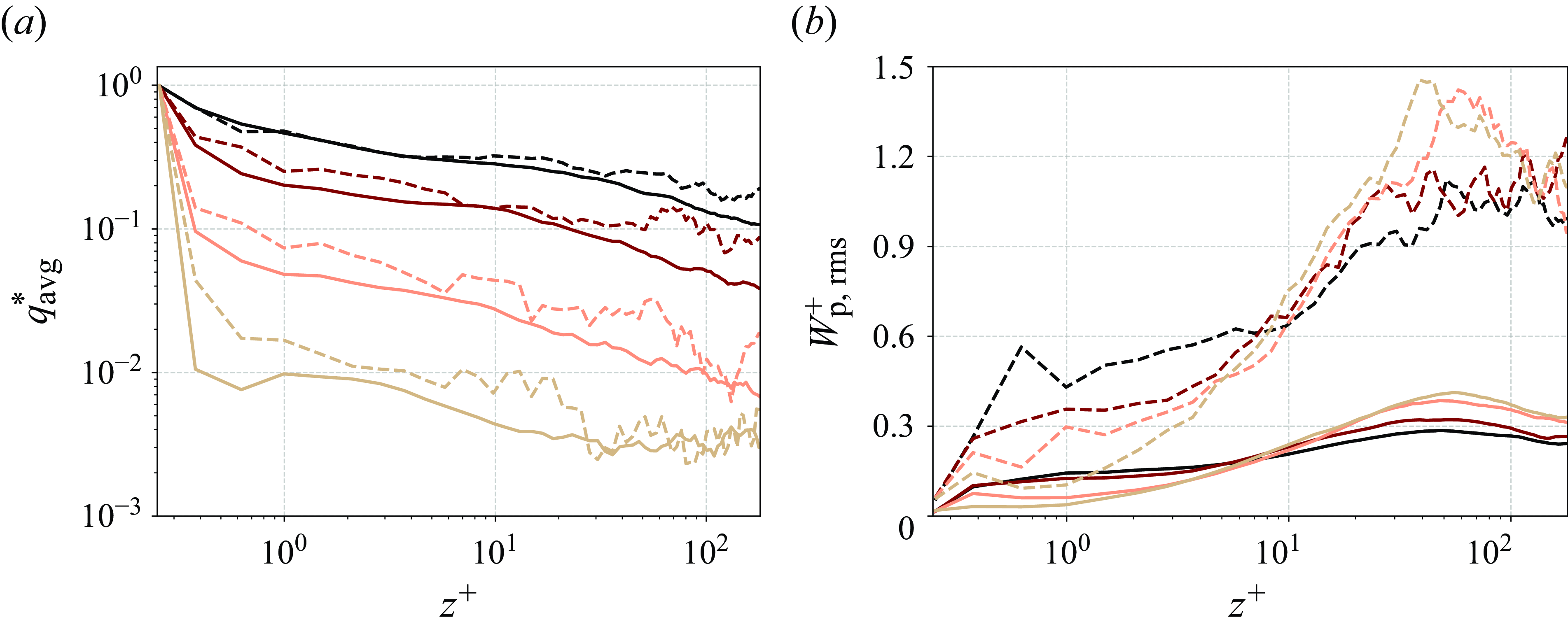
Figure 7. Powder charge distribution along the wall-normal direction in channel and duct flow (a) and r.m.s. wall-normal particle velocities (b). Particle charge is normalized by the equilibrium charge. Shown are the data when the average powder charge is half of the equilibrium charge,
 $q^*_{\textrm {avg}}=0.5$
. The wall-normal profiles along the bisector,
$q^*_{\textrm {avg}}=0.5$
. The wall-normal profiles along the bisector,
 $y^{+\textrm {}}= 180$
, are depicted for duct flow. Solid lines represent channel flow and dashed lines represent duct flow. Colours indicate Stokes number: (
$y^{+\textrm {}}= 180$
, are depicted for duct flow. Solid lines represent channel flow and dashed lines represent duct flow. Colours indicate Stokes number: (![]() )
)
 $St\,=\,37.50$
, (
$St\,=\,37.50$
, (![]() )
)
 $St\,=\,18.75$
, (
$St\,=\,18.75$
, (![]() )
)
 $St\,=\,9.38$
, (
$St\,=\,9.38$
, (![]() )
)
 $St\,=\,4.69$
.
$St\,=\,4.69$
.
The differences between duct and channel flows become more pronounced moving towards the centre of the flow, although substantial differences persist even near the wall. For example, at
 $z^+=10$
, the fluctuations in duct flow are three times greater than in channel flow. This indicates that particles near the wall in ducts are more frequently swept from the near-wall region than in channel flow, where particle mobility near the wall is significantly constrained.
$z^+=10$
, the fluctuations in duct flow are three times greater than in channel flow. This indicates that particles near the wall in ducts are more frequently swept from the near-wall region than in channel flow, where particle mobility near the wall is significantly constrained.
Particles with higher inertia, such as at
 $St$
= 37.50, exhibit significant velocity fluctuations near the wall (
$St$
= 37.50, exhibit significant velocity fluctuations near the wall (
 $z^+ \lt 5$
). In contrast, particles with lower inertia, such as at
$z^+ \lt 5$
). In contrast, particles with lower inertia, such as at
 $St$
= 4.69, demonstrate the lowest fluctuation velocities, indicating their tendency to remain close to the wall for extended periods and experience repetitive collisions. These observations support the anticipated charge profiles, suggesting a more uniform charge distribution in duct flows and higher Stokes numbers.
$St$
= 4.69, demonstrate the lowest fluctuation velocities, indicating their tendency to remain close to the wall for extended periods and experience repetitive collisions. These observations support the anticipated charge profiles, suggesting a more uniform charge distribution in duct flows and higher Stokes numbers.

Figure 8. Magnitude of electric field strength in low-vorticity (
 $||\omega ||$
=
$||\omega ||$
=
 $10^{2}$
 $\mathrm {s}^{-1}$
) and high-vorticity (
$\mathrm {s}^{-1}$
) and high-vorticity (
 $||\omega ||$
=
$||\omega ||$
=
 $10^{3}$
 $\mathrm {s}^{-1}$
) regions for channel and duct flow for particles of
$\mathrm {s}^{-1}$
) regions for channel and duct flow for particles of
 $St =4.69$
. Shown are the data when the average powder charge is half of the equilibrium charge,
$St =4.69$
. Shown are the data when the average powder charge is half of the equilibrium charge,
 $q^*_{\textrm {avg}}=0.5$
.
$q^*_{\textrm {avg}}=0.5$
.
Figure 8 illustrates the probability density distribution of vorticity and electric field for
 $St = 4.69$
in the wall-resolved region, buffer layer and bulk flow. For both channel and duct flow, the electric field strength peaks at the walls and shifts to lower values towards the bulk region. This aligns with the charge profiles shown in figure 7(a), where the average charge of the powder is highest at the walls.
$St = 4.69$
in the wall-resolved region, buffer layer and bulk flow. For both channel and duct flow, the electric field strength peaks at the walls and shifts to lower values towards the bulk region. This aligns with the charge profiles shown in figure 7(a), where the average charge of the powder is highest at the walls.
In the wall-resolved region, channel flow consists solely of high-vorticity zones, while duct flow contains both high- and low-vorticity regions, with low vorticity resulting from the duct corners. The vorticity profiles for channel and duct flows show similar patterns in the buffer layer and bulk flow.
In the channel’s wall-resolved region, electric field strength ranges from 3.49 to
 $ 5.54 \times 10^3 \, \text{V}\,\rm m^-{^1}$
. The maximum occurrence is at a vorticity of
$ 5.54 \times 10^3 \, \text{V}\,\rm m^-{^1}$
. The maximum occurrence is at a vorticity of
 $ 1 \times 10^3 \, \text{s}^{-1}$
and an electric field strength of
$ 1 \times 10^3 \, \text{s}^{-1}$
and an electric field strength of
 $ 3.22 \times 10^1 \, \text{V}\,\rm m^-{^1}$
, followed by a secondary peak at around
$ 3.22 \times 10^1 \, \text{V}\,\rm m^-{^1}$
, followed by a secondary peak at around
 $ 1 \times 10^3 \, \text{V}\,\rm m^-{^1}$
. In duct flow, electric field strength varies from
$ 1 \times 10^3 \, \text{V}\,\rm m^-{^1}$
. In duct flow, electric field strength varies from
 $ 1.34 \times 10^{-1}$
to
$ 1.34 \times 10^{-1}$
to
 $ 4.26 \times 10^3 \, \text{V}\,\rm m^-{^1}$
. Duct flow features regions of low electric field strength in the wall-resolved region, unlike in channel flow. High-vorticity regions in the duct have stronger electric fields, while low-vorticity areas have much weaker electric fields. The highest occurrence in duct flow appears at a vorticity of
$ 4.26 \times 10^3 \, \text{V}\,\rm m^-{^1}$
. Duct flow features regions of low electric field strength in the wall-resolved region, unlike in channel flow. High-vorticity regions in the duct have stronger electric fields, while low-vorticity areas have much weaker electric fields. The highest occurrence in duct flow appears at a vorticity of
 $ 1 \times 10^3 \, \text{s}^{-1}$
and an electric field strength of
$ 1 \times 10^3 \, \text{s}^{-1}$
and an electric field strength of
 $ 9.53 \times 10^1 \, \text{V}\,\rm m^-{^1}$
, with another peak at around
$ 9.53 \times 10^1 \, \text{V}\,\rm m^-{^1}$
, with another peak at around
 $ 6.57 \times 10^2 \, \text{s}^{-1}$
and
$ 6.57 \times 10^2 \, \text{s}^{-1}$
and
 $ 3.38 \, \text{V}\,\rm m^-{^1}$
. Buffer layer and bulk region show similar trends for channel and duct flow.
$ 3.38 \, \text{V}\,\rm m^-{^1}$
. Buffer layer and bulk region show similar trends for channel and duct flow.

Figure 9. Magnitude of electric field strength in low-vorticity (
 $||\omega ||$
=
$||\omega ||$
=
 $10^{2}$
 $\mathrm {s}^{-1}$
) and high-vorticity (
$\mathrm {s}^{-1}$
) and high-vorticity (
 $||\omega ||$
=
$||\omega ||$
=
 $10^{3}$
 $\mathrm {s}^{-1}$
) regions for channel and duct flow for particles of
$\mathrm {s}^{-1}$
) regions for channel and duct flow for particles of
 $St =37.50$
. Shown are the data when the average powder charge is half of the equilibrium charge,
$St =37.50$
. Shown are the data when the average powder charge is half of the equilibrium charge,
 $q^*_{\textrm {avg}}=0.5$
.
$q^*_{\textrm {avg}}=0.5$
.
Figure 9 presents the probability density distribution for
 $St=37.50$
, for the wall-resolved, buffer and bulk regions. For both flow types, electric field strength reaches its peak in the wall-resolved region and diminishes in the bulk, similar to the behaviour seen at
$St=37.50$
, for the wall-resolved, buffer and bulk regions. For both flow types, electric field strength reaches its peak in the wall-resolved region and diminishes in the bulk, similar to the behaviour seen at
 $St=4.69$
. However, compared with
$St=4.69$
. However, compared with
 $St=4.69$
, the lower threshold of electric field strength is higher, which aligns with figure 7(a), indicating higher average powder charges for
$St=4.69$
, the lower threshold of electric field strength is higher, which aligns with figure 7(a), indicating higher average powder charges for
 $St=37.50$
.
$St=37.50$
.
In the wall-resolved region of channel flow, the electric field strength ranges from
 $ 1.56 \times 10^2$
to
$ 1.56 \times 10^2$
to
 $ 4.48 \times 10^3 \, \text{V}\,\rm m^-{^1}$
in high-vorticity areas. In duct flow, both high- and low-vorticity regions are present near the wall, with electric field strengths ranging from
$ 4.48 \times 10^3 \, \text{V}\,\rm m^-{^1}$
in high-vorticity areas. In duct flow, both high- and low-vorticity regions are present near the wall, with electric field strengths ranging from
 $ 1.56 \times 10^1$
to
$ 1.56 \times 10^1$
to
 $ 6.85 \times 10^3 \, \text{V}\,\rm m^-{^1}$
, indicating a broader range compared with channelflow. Compared with
$ 6.85 \times 10^3 \, \text{V}\,\rm m^-{^1}$
, indicating a broader range compared with channelflow. Compared with
 $St = 4.69$
, the electric field strength is not reduced in low-vorticity regions and exhibits a more uniform distribution across varying vorticity levels. This suggests that the distribution of charged particles along the wall significantly differs with different Stokes numbers.
$St = 4.69$
, the electric field strength is not reduced in low-vorticity regions and exhibits a more uniform distribution across varying vorticity levels. This suggests that the distribution of charged particles along the wall significantly differs with different Stokes numbers.
In the buffer layer, both flow types exhibit regions of high and low vorticity. In the high-vorticity region, electric field strength is higher, with channel flow demonstrating higher values than duct flow.
In the bulk region, channel flow maintains only stronger electric fields in high-vorticity areas, while duct flow shows a uniform electric field distribution across vorticity levels.
4.2. Effects of electrostatic charge on fluid and particle dynamics
In this section, we investigate the impact of triboelectric charging on powder flow dynamics. Electrostatic forces significantly influence particle behaviour and distribution within the domain. This interaction, in turn, affects the fluid phase and alters the overall flow characteristics.

Figure 10. Normalized particle concentration profiles of uncharged and charged duct flow. For the charged case, the average powder charge in the duct is half of the equilibrium charge,
 $q^*_{\textrm {avg}}=0.5$
. Due to symmetry, only one quadrant of the squareduct is shown.
$q^*_{\textrm {avg}}=0.5$
. Due to symmetry, only one quadrant of the squareduct is shown.
Figure 10 illustrates concentration profiles within duct flow, comparing scenarios with uncharged particles to those where the powder has reached half of its equilibrium charge (
 $q^*_{\textrm {avg}}=0.5$
). In all scenarios, particles accumulate at the duct walls, with fewer particles found at the centre of the duct. The Stokes number of the particles affects the specific locations of this accumulation along the wall.
$q^*_{\textrm {avg}}=0.5$
). In all scenarios, particles accumulate at the duct walls, with fewer particles found at the centre of the duct. The Stokes number of the particles affects the specific locations of this accumulation along the wall.
For uncharged particles, those with
 $St = 4.69$
accumulate at the wall bisectors and within therange
$St = 4.69$
accumulate at the wall bisectors and within therange
 $z^+ = 20$
to
$z^+ = 20$
to
 $z^+ = 60$
. Particles with
$z^+ = 60$
. Particles with
 $St = 9.38$
collect at the wall bisectors and between
$St = 9.38$
collect at the wall bisectors and between
 $z^+ = 10$
and
$z^+ = 10$
and
 $z^+ = 60$
. In contrast, particles with
$z^+ = 60$
. In contrast, particles with
 $St = 18.75$
and
$St = 18.75$
and
 $St = 37.50$
concentrate at the corners of the duct.
$St = 37.50$
concentrate at the corners of the duct.
The preferred accumulation of particles is directly related to the interplay between particles’ inertia and the secondary flow structures. Particles with higher inertia,
 $St$
= 18.75 and 37.50, accumulate mainly in the stagnation region (corners). This occurs because, beyond a specific point near the corner where the secondary flow changes direction, the secondary flow velocities arenot strong enough to maintain the motion of high-inertia particles parallel to the walls, leading them to accumulate more within the stagnation region (Wang et al. Reference Wang, Fairweather, Mortimer, Zhao and Yao2020). In contrast, low-inertia particles,
$St$
= 18.75 and 37.50, accumulate mainly in the stagnation region (corners). This occurs because, beyond a specific point near the corner where the secondary flow changes direction, the secondary flow velocities arenot strong enough to maintain the motion of high-inertia particles parallel to the walls, leading them to accumulate more within the stagnation region (Wang et al. Reference Wang, Fairweather, Mortimer, Zhao and Yao2020). In contrast, low-inertia particles,
 $St$
= 4.69, closely follow the secondary flow, avoiding collection at the corner.
$St$
= 4.69, closely follow the secondary flow, avoiding collection at the corner.
When particles acquire charge, they undergo significant changes due to the electrostatic forces exerted by mirror charges on the walls. Charged particles also generate electric fields in their vicinity, capable of repelling other charged particles. These interactions influence their trajectories and alter the resulting particle concentration profiles.
Results show that, when particles are charged, their accumulation at the wall increases across all scenarios. However, the distribution along the wall varies. In the uncharged case, with
 $St$
= 4.69, particles accumulate primarily at the wall bisectors and within the range
$St$
= 4.69, particles accumulate primarily at the wall bisectors and within the range
 $z^+ = 20$
to
$z^+ = 20$
to
 $z^+ = 60$
. Particles with
$z^+ = 60$
. Particles with
 $St = 9.38$
collect at the wall bisectors and between
$St = 9.38$
collect at the wall bisectors and between
 $z^+ = 10$
and
$z^+ = 10$
and
 $z^+ = 60$
. Upon charging, accumulation becomes solely concentrated at the wall bisectors. Compared with
$z^+ = 60$
. Upon charging, accumulation becomes solely concentrated at the wall bisectors. Compared with
 $St$
= 4.69, the profile along the wall is more uniform when
$St$
= 4.69, the profile along the wall is more uniform when
 $St$
= 9.38. In cases where
$St$
= 9.38. In cases where
 $St$
= 18.75 and 37.50, charged particles accumulate significantly at the corners of the duct. This increased concentration is due to electrostatic forces from mirror charges on both walls, which attract particles towards these corners.
$St$
= 18.75 and 37.50, charged particles accumulate significantly at the corners of the duct. This increased concentration is due to electrostatic forces from mirror charges on both walls, which attract particles towards these corners.
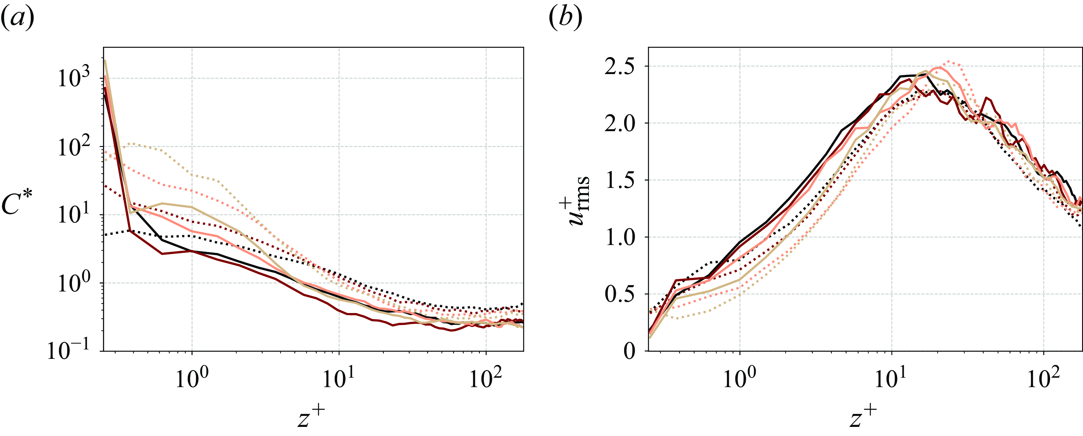
Figure 11. Normalized particle concentration profiles (a) and r.m.s. streamwise fluid velocity (b) for uncharged and charged duct flow. The wall-normal profiles along the bisector,
 $y^{+\textrm {}}= 180$
, are depicted for duct flow. The uncharged case is shown by dotted lines while the charged case is shown by solid lines. For the charged case, the average powder charge in the domain is half of the equilibrium charge,
$y^{+\textrm {}}= 180$
, are depicted for duct flow. The uncharged case is shown by dotted lines while the charged case is shown by solid lines. For the charged case, the average powder charge in the domain is half of the equilibrium charge,
 $q^*_{\textrm {avg}}=0.5$
, for duct flow. Colours indicate Stokes number: (
$q^*_{\textrm {avg}}=0.5$
, for duct flow. Colours indicate Stokes number: (![]() )
)
 $St\,=\,37.50$
, (
$St\,=\,37.50$
, (![]() )
)
 $St\,=\,18.75$
, (
$St\,=\,18.75$
, (![]() )
)
 $St\,=\,9.38$
, (
$St\,=\,9.38$
, (![]() )
)
 $St\,=\,4.69$
.
$St\,=\,4.69$
.
Figure 11(a) shows the concentration profiles along the bisector,
 $y^+=\,180$
, of the duct for charged and uncharged particles. In all scenarios, particles accumulate the most at the duct walls, with the most pronounced accumulation observed for
$y^+=\,180$
, of the duct for charged and uncharged particles. In all scenarios, particles accumulate the most at the duct walls, with the most pronounced accumulation observed for
 $St$
= 4.69. Notably, in the uncharged case, the accumulation for
$St$
= 4.69. Notably, in the uncharged case, the accumulation for
 $St$
= 4.69 occurs not directly at the wall but at
$St$
= 4.69 occurs not directly at the wall but at
 $z^+\,=\,0.38$
. However, when particles are charged, they accumulate directly at the wall. This shift demonstrates that electrostatic forces have a stronger influence than aerodynamic forces in determining particle location. In other words, the attractive electrostatic forces from the mirror charges at the wall bring particles from the near-wall region directly to the wall.
$z^+\,=\,0.38$
. However, when particles are charged, they accumulate directly at the wall. This shift demonstrates that electrostatic forces have a stronger influence than aerodynamic forces in determining particle location. In other words, the attractive electrostatic forces from the mirror charges at the wall bring particles from the near-wall region directly to the wall.
As Stokes number increases, the concentration at the duct wall decreases. This trend is similar for charged and uncharged particles, although less pronounced for charged particles. For uncharged particles, the wall concentration is around 20 times higher for
 $St$
= 4.69 compared with
$St$
= 4.69 compared with
 $St$
= 37.50. When particles are charged, this concentration ratio reduces to 4. Therefore, electrostatic forces dominate aerodynamic forces in the near-wall region.
$St$
= 37.50. When particles are charged, this concentration ratio reduces to 4. Therefore, electrostatic forces dominate aerodynamic forces in the near-wall region.
When particles gain charge, there is a significant increase in their accumulation directly at the wall. For instance, the particle concentration at the wall increased approximately 30 times for
 $St$
= 4.69 compared with the uncharged condition. Similarly, for
$St$
= 4.69 compared with the uncharged condition. Similarly, for
 $St$
= 9.38, 18.75 and 37.50, the concentration increased by 10, 20 and 100 times, respectively. Consequently, this wall accumulation reduces particle concentration at the centre of the duct.
$St$
= 9.38, 18.75 and 37.50, the concentration increased by 10, 20 and 100 times, respectively. Consequently, this wall accumulation reduces particle concentration at the centre of the duct.
Figure 11(b) displays the r.m.s. fluid velocity in the streamwise direction for both the uncharged and charged cases.
When charged, particles tend to move away from the centre of the duct. This migration reduces the number of particles in the centre, which, in turn, allows for higher turbulence and fluctuations in the fluid velocity. As a result, the r.m.s. fluid velocity, which measures the intensity of these fluctuations, increases at the centre of the duct.
In contrast, at the duct walls, the increase in particle concentration due to charging has the opposite effect. The high concentration of particles at the wall can dampen or suppress the turbulence in this region. This results in a decrease in the r.m.s. fluid velocity near the wall, as the increased particle presence reduces the intensity of turbulent fluctuations in that area. These findings align with the research of Zhang et al. (Reference Cui, Zhang and Zheng2024) on DNS of turbulent channel flow, which showed that the r.m.s. of streamwise-fluctuating velocity decreases with particle presence and is further suppressed for charged particles, indicating that interparticle electrostatic forces inhibit turbulence.
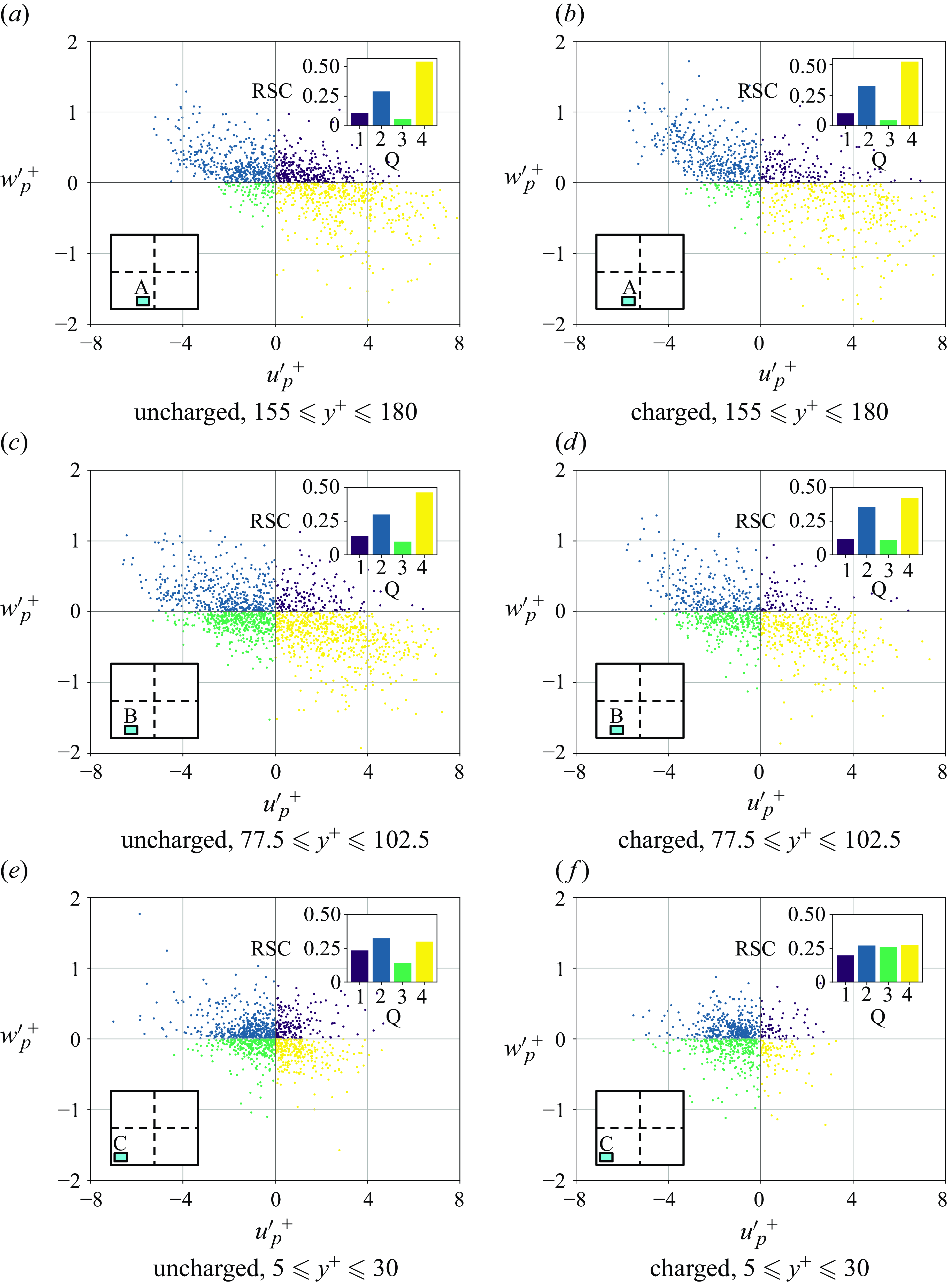
Figure 12. Quadrant analysis and Reynolds stress contribution (RSC; upper-right inset) of uncharged and charged duct flow. The Stokes number is
 $St$
= 4.69. Shown is the lower-left quarter of the duct in the near-wall region (
$St$
= 4.69. Shown is the lower-left quarter of the duct in the near-wall region (
 $5\leqslant z^{+\textrm {}}\leqslant 30$
). For the charged case, the average powder charge is half of the equilibrium charge,
$5\leqslant z^{+\textrm {}}\leqslant 30$
). For the charged case, the average powder charge is half of the equilibrium charge,
 $q^*_{\textrm {avg}}=0.5$
.
$q^*_{\textrm {avg}}=0.5$
.
Figure 12 presents the quadrant analysis of duct flow, and the contribution to Reynolds stress
 $\langle \mathit {u}'_{\mathrm {p}}\mathit {w}'_{\mathrm {p}} \rangle$
in the lower-left quarter close to the wall region (
$\langle \mathit {u}'_{\mathrm {p}}\mathit {w}'_{\mathrm {p}} \rangle$
in the lower-left quarter close to the wall region (
 $5\leqslant z^{+\textrm {}}\leqslant 30$
). The analysis covers three distinct areas:
$5\leqslant z^{+\textrm {}}\leqslant 30$
). The analysis covers three distinct areas:
 $155 \leqslant y^+ \leqslant 180$
(region A),
$155 \leqslant y^+ \leqslant 180$
(region A),
 $77.5 \leqslant y^+ \leqslant 102.5$
(region B) and
$77.5 \leqslant y^+ \leqslant 102.5$
(region B) and
 $5 \leqslant y^+ \leqslant 30$
(region C). The contribution to Reynolds stress for each quadrant is calculated as
$5 \leqslant y^+ \leqslant 30$
(region C). The contribution to Reynolds stress for each quadrant is calculated as
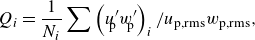 \begin{equation} Q_{i}=\frac {1}{N_{i}}\sum \left ( u'_{\!\!\textrm {p}}w'_{\!\!\textrm {p}} \right )_{i}/u_{\textrm {p,rms}}w_{\textrm {p,rms}}, \end{equation}
where
 $Q_{i}$
is the contribution from the
$Q_{i}$
is the contribution from the
 $i$
th quadrant and
$i$
th quadrant and
 $N_{i}$
is the number of
$N_{i}$
is the number of
 $i$
th quadrant events. Reynolds stress contributions are given as a percentage of the total contributions.
$i$
th quadrant events. Reynolds stress contributions are given as a percentage of the total contributions.
Here Q2 (ejections) and Q4 (sweeps) events arise from interactions of counter-rotating vortices in wall-bounded turbulent flows. In contrast, Q1 and Q3 events do not directly correspond to specific turbulent structures in flows with a single inhomogeneous direction. Nevertheless, Q1 and Q3 events significantly influence turbulence dynamics in turbulent duct flows (Huser & Biringen Reference Huser and Biringen1993; Fornari et al. Reference Fornari, Kazerooni, Hussong and Brandt2018). Thus, while turbulence patterns in a square duct are generally similar to those in a wall-bounded turbulent channel flow, the presence of secondary flows introduces notable differences.
Figure 12 shows that overall, Q2 (ejections) and Q4 (sweeps) events contribute significantly to Reynolds stress. In region A, Q4 events are responsible for half of the contribution to Reynolds stress alone. However, notable increases in the contributions from Q1 and Q3 events appear as we move towards region C. Specifically, Q3 events contribute 5.8 % in region A, 9.8 % in region B and 14.2 % in region C. In region C, Q3 events are driven by interactions between Q2 events from horizontal and vertical walls, which redirect the ejection flow towards the perpendicular wall (Huser & Biringen Reference Huser and Biringen1993). Similarly, Q1 event contributions increase from 11.1 % in region A to 14.0 % in region B and to 23.4 % in region C.
In contrast, Q4 events are most significant in region A and diminish towards the corners, explaining particle accumulation in regions A and B. The Q4 contributions to Reynolds stress are 54.1 % in region A, 46.3 % in region B and 30.0 % in region C. The Q2 events are not significantly influenced by proximity to the wall but are slightly reduced in region A.
Upon charging, some particles deposit directly at the walls, which reduces the number of data points. Charging significantly alters the quadrant analysis, particularly in region C, while its impact in regions A and B is relatively minor. Upon charging, contributions become almost homogeneously distributed across the quadrants in region C. This may stem from the concentrated effect of electrostatic forces at the corners, where attractive forces from image charges on both vertical and horizontal walls amplify the overall electrostatic interaction with particles. Specifically, the contribution from Q3 events in region C nearly doubles from 14.2 % to 25.9 %. Interestingly, charging also suppresses Q1, Q2 and Q4 events. The Q4 contributions decrease significantly from 33.0 % to 26.0 %, while Q2 contributions decrease from 32.5 % to 27.0 %, and Q1 contributions from 23.4 % to 19.8 %.

Figure 13. Normalized particle concentration profiles (a) and r.m.s. streamwise fluid velocity (b) for uncharged and charged channel flow. The uncharged case is shown by dotted lines while the charged case is shown by solid lines. For the charged case, the average powder charge in the domain is half of the equilibrium charge,
 $q^*_{\textrm {avg}}=0.5$
. Colours indicate Stokes number: (
$q^*_{\textrm {avg}}=0.5$
. Colours indicate Stokes number: (![]() )
)
 $St\,=\,37.50$
, (
$St\,=\,37.50$
, (![]() )
)
 $St\,=\,18.75$
, (
$St\,=\,18.75$
, (![]() )
)
 $St\,=\,9.38$
, (
$St\,=\,9.38$
, (![]() )
)
 $St\,=\,4.69$
.
$St\,=\,4.69$
.
Figure 13(a) shows normalized particle concentration in the channel flow for uncharged and charged powder. The concentration profiles in channel flow show a similar pattern to those in duct flow. Particles are accumulated at the channel walls in uncharged and charged cases. As particles become charged, there is a significant rise in concentration at the wall, similar to duct flow. In the charged case, particle concentration directly at the channel walls is less affected by Stokes number than in duct flow. In both duct and channel flow, particle concentration at the centre decreases due to the attraction of charged particles to the walls.
Figure 13(b) shows the r.m.s. of fluid velocity in the streamwisedirection for both the uncharged and charged cases. Overall, fluid velocity fluctuations in the streamwise direction in channel flow are less pronounced than in duct flow. Similar to duct flow, when particles are charged, fluctuations at the wall decrease due to particle accumulation, while fluctuations at the centre increase as particles move away from this region.
Thus, while the overall intensity of fluctuations in channel flow is lower than in duct flow, the effect of charging particles on the distribution of these fluctuations remains consistent between the two flow types.
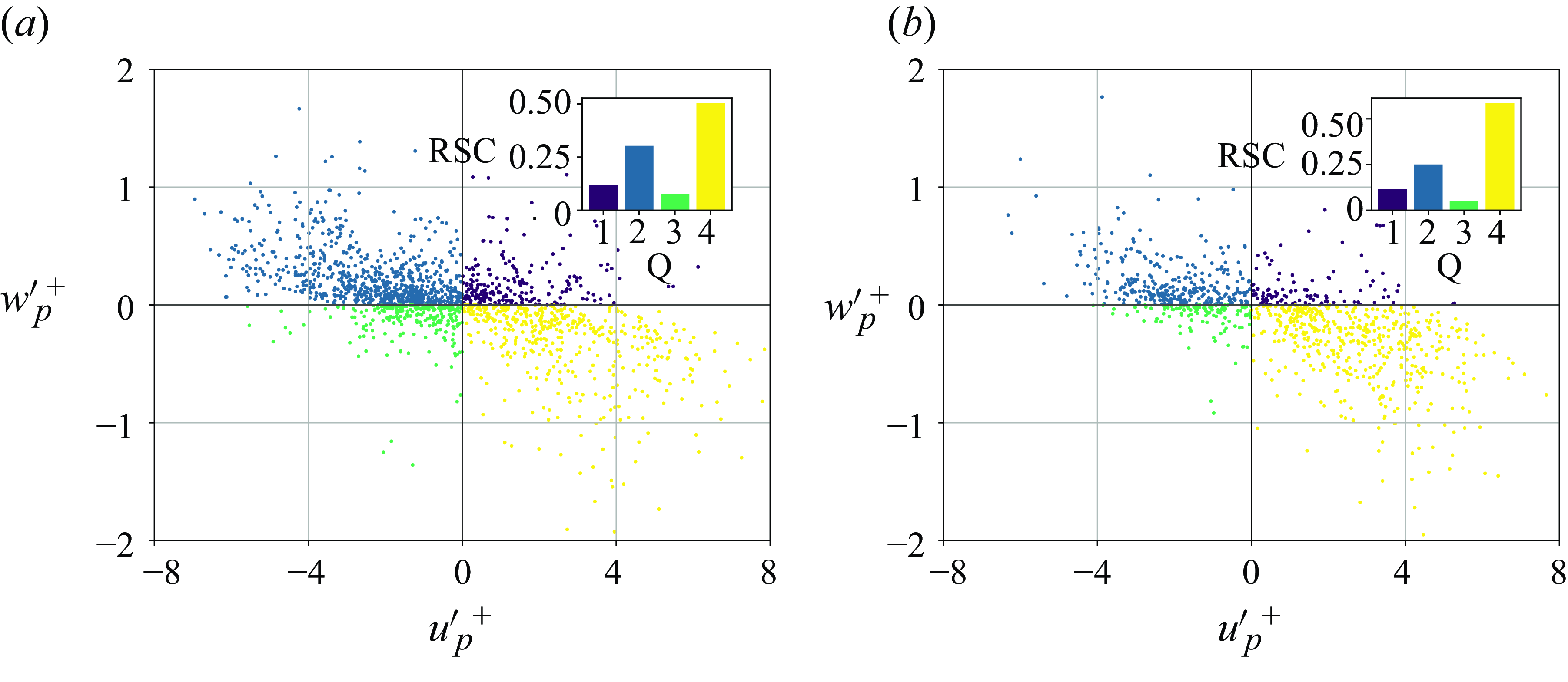
Figure 14. Quadrant analysis and Reynolds stress contribution (RSC; upper-rightinset) of uncharged (a) and charged (b) channel flow. Shown is the near-wall region (
 $5\leqslant z^{+\textrm {}}\leqslant 30$
). Stokes number is
$5\leqslant z^{+\textrm {}}\leqslant 30$
). Stokes number is
 $St$
= 4.69. For the charged case, the average powder charge is half of the equilibrium charge,
$St$
= 4.69. For the charged case, the average powder charge is half of the equilibrium charge,
 $q^*_{\textrm {avg}}=0.5$
.
$q^*_{\textrm {avg}}=0.5$
.
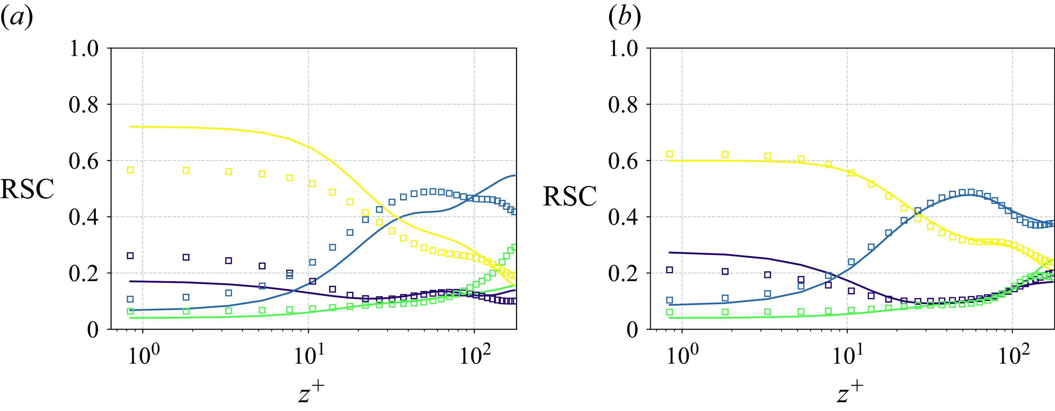
Figure 15. Wall-normal profiles of contribution to particle Reynolds stress (RSC) for (a) channel flow and (b) duct flow. The wall-normal profiles along the bisector,
 $y^{+\textrm {}}= 180$
, are depicted for duct flow. Lines represent the chargedcase and data points represent the uncharged case. For the charged case, the average powder charge in the domain is half of the equilibrium charge,
$y^{+\textrm {}}= 180$
, are depicted for duct flow. Lines represent the chargedcase and data points represent the uncharged case. For the charged case, the average powder charge in the domain is half of the equilibrium charge,
 $q^*_{\textrm {avg}}=0.5$
. Colours indicate different quadrants: (
$q^*_{\textrm {avg}}=0.5$
. Colours indicate different quadrants: (![]() ) Q1, (
) Q1, (![]() ) Q2, (
) Q2, (![]() ) Q3, (
) Q3, (![]() ) Q4.
) Q4.
Figure 14 shows the quadrant analysis of channel flow at the channel wall for charged and uncharged cases. The frequency of Q2 and Q4 events is substantially higher compared with Q1 and Q3 events. Here 80 % of the Reynolds stress contribution comes from Q2 (ejections) and Q4 (sweeps) events. Specifically, Q4 events contribute 50 %, while Q2 events account for 30 %. This indicates that these turbulent events, characterized by the outward and inward movement of fluid near the walls, play a dominant role in the overall turbulence dynamics of a channel flow. In contrast, Q1 and Q3 events contribute less to Reynolds stress in the channel flow. The Q1 events account for 11.5 % of the Reynolds stress, and Q3 events contribute 4.9 %.
As particles become charged, they accumulate on the walls, resulting in a decrease in the number of data points. Regarding Reynolds stress contributions, Q2 and Q4 events exhibit the most significant changes. Specifically, the contribution from Q2 events decreases from 30 % to 25 %, while the contribution from Q4 events increases from 50 % to 58 %. This increase in Q4 events, which involve the sweeping of particles towards the wall, is attributed to the enhanced electrostatic attraction that charged particles experience from the wall. Conversely, the decrease in Q2 events, which involve the ejection of particles away from the wall, results from the dominance of electrostatic forces over the turbulent structures responsible for these ejections. In contrast, Q1 and Q3 events remain relatively unaffected by charging, unlike in duct flow.
Figure 15 shows wall-normal profiles of the contribution to particle Reynolds stress in channel and duct flows, comparing charged and uncharged cases. When uncharged, contribution profiles from different quadrants demonstrate consistent patterns between channel and duct flows, with slight variations in magnitude. However, the influence of particle charge on the profiles varies significantly across the two flow types. Generally, the changes in the distribution of particle Reynolds stress contributions upon charging are less pronounced in duct flow compared with channel flow. This difference may be due to the presence of secondary flow structures in ducts, which can dominate the effects of electrostatic forces. In contrast, channel flow lacks these secondary structures, leading to more significant changes in the particle behaviour when charged.
In both channel and duct flows, the near-wall region (
 $z^+\lt 30$
) is dominated by Q4 events, with approximately 0.6 of the total contributions. Following this, Q1 events account for about 0.2, while contributions from Q2 and Q3 events are around 0.1. In the turbulent region (
$z^+\lt 30$
) is dominated by Q4 events, with approximately 0.6 of the total contributions. Following this, Q1 events account for about 0.2, while contributions from Q2 and Q3 events are around 0.1. In the turbulent region (
 $z^+\gt 30$
), contributions from Q2 events significantly exceed those from Q4 events, with Q4 contributions decreasing to approximately 0.2 and Q2 contributions rising to about 0.4. At the centre (
$z^+\gt 30$
), contributions from Q2 events significantly exceed those from Q4 events, with Q4 contributions decreasing to approximately 0.2 and Q2 contributions rising to about 0.4. At the centre (
 $z^+=180$
), Q3 events reach 0.3, surpassing the contributions from Q4 in the channel flow while it stays around 0.2 for duct flow.
$z^+=180$
), Q3 events reach 0.3, surpassing the contributions from Q4 in the channel flow while it stays around 0.2 for duct flow.
Upon charging, in the near-wall region, the contribution to particle Reynolds stress from Q4 events increases in channel flow but slightly decreases in duct flow. Conversely, Q1 events show a decrease in channel flow and a slight increase in duct flow. The Q2 events also decrease in channel flow, with no significant change in duct flow. These observations in channel flow indicate that electrostatic forces substantially affect particle dynamics. The increased contribution from Q4 events suggests that particles are attracted towards the wall due to mirror charges, reducing the contributions from Q1 and Q2 events. In duct flow, such behaviour is absent, suggesting that secondary flow structures have a greater influence than electrostatic forces.
Charging significantly affects contributions at the centre of channel flow. Upon charging, contributions from Q1 and Q2 events increase, while those from Q3 and Q4 decrease. The decrease in contributions from Q3 and Q4 events results from particles depositing on the channel walls upon charging. With fewer particles present at the centre, the number of particles moving towards the wall decreases, which increases the relative contribution from other quadrants towards the centre. In duct flow, the effect of charging on quadrant contributions is less pronounced: Q2 remains unchanged between charged and uncharged states, Q1 and Q4 slightly reduce and Q3 increases.
Figure 16 shows the one-dimensional energy spectra for channel and duct flow with charged and uncharged particles. In both flow types, turbulent kinetic energy in the streamwise direction increases when particles are charged. In duct flow, this increase is more pronounced compared with channel flow. In channel flow, turbulent kinetic energy is higher for the charged case at low
 $(k/k_{\mathrm {d}} = 10^{-2})$
and intermediate
$(k/k_{\mathrm {d}} = 10^{-2})$
and intermediate
 $(k/k_{\mathrm {d}} = 10^{-1})$
wavenumbers, while in duct flow, it spans low, intermediate and high wavenumbers
$(k/k_{\mathrm {d}} = 10^{-1})$
wavenumbers, while in duct flow, it spans low, intermediate and high wavenumbers
 $(k/k_{\mathrm {d}} \gt 10^{-1})$
. In channel flow, the kinetic energy for the charged case falls below that for the uncharged case for high wavenumbers
$(k/k_{\mathrm {d}} \gt 10^{-1})$
. In channel flow, the kinetic energy for the charged case falls below that for the uncharged case for high wavenumbers
 $k/k_{\mathrm {d}} =0.2$
. Additionally, in duct flow, turbulent kinetic energy in the spanwise and wall-normal directions also increases with particle charging, whereas it decreases in channel flow.
$k/k_{\mathrm {d}} =0.2$
. Additionally, in duct flow, turbulent kinetic energy in the spanwise and wall-normal directions also increases with particle charging, whereas it decreases in channel flow.
The increase in turbulent kinetic energy, when particles are charged, is caused by particle migration from the centre to the walls, where they deposit due to the effect of electrostatic forces, as explained by figures 11 and 13. This migration reduces particle interference with large eddies in the centre, leading to an increase in turbulent kinetic energy. Similar findings have been reported in DNS studies of turbulent pipe flows (Gupta, Clercx & Toschi Reference Gupta, Clercx and Toschi2018), which compare the one-dimensional energy spectra of laden and unladen flows.
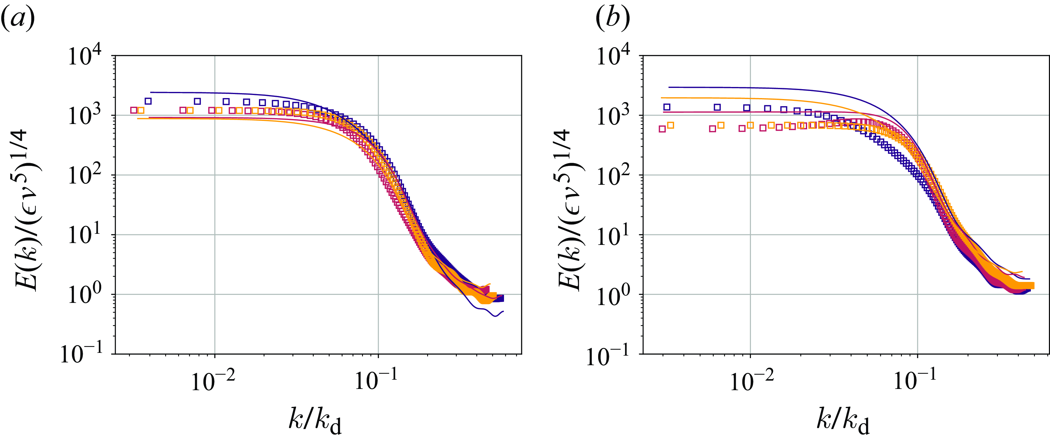
Figure 16. One-dimensional energy spectra for (a) channel flow and (b) duct flow, normalized by energy dissipation
 $\epsilon$
and kinematic viscosity
$\epsilon$
and kinematic viscosity
 $\nu$
, plotted against wavenumber
$\nu$
, plotted against wavenumber
 $k$
normalized by the Kolmogorov length scale
$k$
normalized by the Kolmogorov length scale
 $k_{\mathrm {d}}$
. The spectra are plotted for
$k_{\mathrm {d}}$
. The spectra are plotted for
 $y^+=180$
and
$y^+=180$
and
 $z^+=180$
. Lines represent the chargedcase and the data points represent the uncharged case. For the charged case, the average powder charge is half of the equilibrium charge,
$z^+=180$
. Lines represent the chargedcase and the data points represent the uncharged case. For the charged case, the average powder charge is half of the equilibrium charge,
 $q^*_{\textrm {avg}}=0.5$
. Colours show different velocity components of fluid flow: (
$q^*_{\textrm {avg}}=0.5$
. Colours show different velocity components of fluid flow: (![]() )
)
 $u$
, (
$u$
, (![]() )
)
 $v$
, (
$v$
, (![]() )
)
 $w$
.
$w$
.
5. Conclusions
In this study, we investigated how flow patterns impact the charging of powder flows. To separate this effect from the complex nature of particle charging, we employed a generic charging model based solely on the precharge of the particles. As a result, powder charging is affected by particle trajectories, which are shaped by the surrounding flow. Specifically, powder charging depends on two main factors: the frequency of particle charging at the walls and the rate at which charge spreads from the walls to the bulk via particle-bound transport.
Our study highlights the effect of secondary flow structures on powder charging rates and charge distribution. We revealed that powder charges faster in duct flow than in channel flow carrying the same particles. Furthermore, the charge is more uniformly distributed across the duct cross-section than across the channel cross-section. This is due to the secondary flow structures in duct flows, which accelerate the particles to the walls. As a result, in duct flow, collision rates are higher, which means that charging events are more frequent. But more importantly, secondary flows also bring particles to the corners, then to bisectors and finally to the centre, promoting particle-bound charge transfer. Therefore, the charge transferred during each collision event is higher in duct flow. Conversely, in channel flow, particles tend to trap near the wall and make repeating collisions, limiting the charge transferred during each collision event.
Stokes number of particles significantly impacts their charging behaviour in both channel- and duct-flow scenarios. Typically, particles with higher Stokes number tend to move uniformly along the wall-normal direction, resulting in faster and more uniform charging. However, in duct flow, high-inertia particles tend to accumulate at the corners, resulting in some particles remaining uncharged.
Upon charging, electrostatic forces draw more particles towards the wall, leading to higher wall accumulation at the walls and fewer particles in the centre for both channel and duct flows. This shift in particle distribution has impacts on the fluid phase. Due to the accumulation of particles, streamwise fluid velocity fluctuations were reduced at the walls while they increased at the centre.
The results of this study demonstrate the fundamental influence of flow scenarios on the charging pattern of two-phase flows. Understanding these influences gives us new insights into how we can control the charging process in handling powder flows. The capability to control or limit the accumulation of electric charging of powder flows would enable a better understanding of environmental processes, optimizing industrial devices and mitigating hazards to their operational safety.
Funding.
This research received financial support from the European Research Council (ERC) under the European Union’s Horizon 2020 research and innovation programme (grant agreement no. 947606 Pow-FEct).
Declaration of interests.
The authors report no conflict of interest.


