Introduction
The dominant feature of the South Atlantic sector of the Southern Ocean is the Antarctic Circumpolar Current (ACC) (Orsi et al. Reference Orsi, Whitworth and Nowlin1995, Rintoul et al. Reference Rintoul, Hughes and Olbers2001), which is a strong zonal current that flows eastward driven mostly by the Southern Hemisphere westerlies (Russell et al. Reference Russell, Dixon, Gnanadesikan, Stouer and Toggweiler2006, Toggweiler Reference Toggweiler2009). Observations show the ACC mean transport is between 118 and 146 Sverdrups (Sv) through the Drake Passage (Whitworth Reference Whitworth1983, Orsi et al. Reference Orsi, Whitworth and Nowlin1995, Meredith et al. Reference Meredith, Woodworth, Chereskin, Marshall, Allison and Bigg2011). The South Atlantic has four main fronts, although many more have been identified, depending on how they are defined, as discussed by Freeman & Lovenduski (Reference Freeman and Lovenduski2016). These can be seen together with the major South Atlantic currents, schematically in Fig. 1. They are, from north to south, the Subtropical Front (STF), the sub-Antarctic Front (SAF) and the Antarctic Polar Front (PF). The currents depicted are the Brazil Current (BC), the South Atlantic Current (SAC), the Benguela Current (BE) and the South Equatorial Current (SEC).
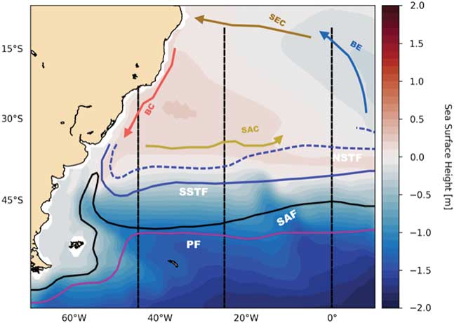
Fig. 1 Schematic representation of the South Atlantic circulation with the Brazil Current (BC), South Equatorial Current (SEC) and South Atlantic Current (SAC). The main Southern Ocean fronts are the Subtropical Front (STF) with its southern (SSTF) and northern (NSTF) limit marked, the Sub Antarctic Front (SAF) and Polar Front (PF).
There are many criteria to distinguish Southern Ocean fronts. Some are based on hydrographical properties (Orsi et al. Reference Orsi, Whitworth and Nowlin1995) while others are based on gradients of Sea Surface Height (SSH) or Sea Surface Temperature (SST) (Dong et al. Reference Dong, Sprintall and Gille2006, Sallée et al. Reference Sallée, Speer and Morrow2008, Sokolov & Rintoul Reference Sokolov and Rintoul2009). Understanding the latitudinal changes and variability of these fronts has been an important and active area of research because of the implications for water mass formation, the uptake and transport of heat and carbon dioxide, and biological productivity. All of these factors have a significant impact on climate change (Downes et al. Reference Downes, Budnick, Sarmiento and Farneti2011, Fan et al. Reference Fan, Deser and Schneider2014).
Rintoul et al. (Reference Rintoul, Hughes and Olbers2001), Russell et al. (Reference Russell, Dixon, Gnanadesikan, Stouer and Toggweiler2006), Fyfe et al. (Reference Fyfe, Saenko, Zickfeld, Eby and Weaver2007), Toggweiler (Reference Toggweiler2009), Gent & Danabasoglu (Reference Gent and Danabasoglum2011) and others discuss how important the westerlies are in driving the ACC system and how climate change has been changing the winds that in turn impact the ACC dynamics. The westerly winds influence not only the position and transport of the ACC but also impact the rate of water mass production and the transformation of Antarctic Intermediate Water (e.g. Santoso & England (Reference Santoso and England2004), Wainer et al. (Reference Wainer, Goes, Murphy and Brady2012)).
The focus of this study is the South Atlantic sector of the Southern Ocean from 30–70°S. The circulation near the surface is wind driven (Stramma & England Reference Stramma and England1999). The Benguela Current that flows northward along the African coast off the Cape of Good Hope is the limit of the subtropical gyre in the eastern Atlantic. The Benguela Current splits into two branches: one continues its northward flow along the coast and the other veers to the west to form the South Equatorial Current. To the south, the subtropical gyre is limited by the South Atlantic Current. Waters from the Antarctic Intermediate Water and the sub-Antarctic Mode Waters are contained in the South Atlantic Current (McCartney Reference McCartney1977, Rintoul et al. Reference Rintoul, Hughes and Olbers2001). Also, part of the regional current system is the Falkland (Malvinas) Current, which is the northward flowing branch of the ACC into the Atlantic. At about 40°S it encounters the Brazil Current. North of the sub-Antarctic Front (SAF) the sub-Antarctic Mode Waters can be found. The temperature of this water mass is about 14 °C in the western South Atlantic just north of the SAF, which is also just east of the Falkland Current retroflection (Talley Reference Talley, Pickard, Emery and Swift2011).
The South Atlantic sector of the Southern Ocean encompasses the region where the sub-Antarctic Mode Water meets the cooler sub-Antarctic surface waters. It is there where the major frontal system that separates the subtropical from the polar circulation is found. The sub-Antarctic Mode Water together with surface waters south of the sub-Antarctic Front are sources for Antarctic Intermediate Water, which sits within the Polar Front (PF) region. The PF is where the cold, fresh Antarctic surface waters subduct beneath warmer, saltier sub-Antarctic waters. The PF is characterized by strong gradients in temperature, salinity and density (Orsi et al. Reference Orsi, Whitworth and Nowlin1995).
The Southern Hemisphere westerlies have been observed to intensify and move southward over the latter part of the 20th century. It is generally agreed that this is caused by the increase in greenhouse gases and reduction in stratospheric ozone concentrations (Polvani et al. Reference Polvani, Waugh, Correa and Son2011, Kim & Orsi Reference Kim and Orsi2014, Gent Reference Gent2016). This paper addresses the question of how this change in the westerlies has affected the circulation of the South Atlantic, and whether the various fronts have changed latitude. This is done by evaluating the results from a ten-member ensemble of simulations using the Community Earth System Model, Last Millennium Ensemble (CESM-LME). The behaviour of the South Atlantic sector of the Southern Ocean is characterized over two periods: between the years 1050–1950 and the years 1970–2000.
The Community Earth System Model - CESM
The version of the CESM used in this study is fully documented in Kay et al. (Reference Kay, Deser, Phillips, Mai, Hannay and Strand2015). The horizontal resolution in the atmosphere and land components is 2°. The horizontal resolution in the ocean and sea-ice components is 1°. The ocean component has 60 levels, which are 10 m thick in the upper ocean, and is documented in Danabasoglu et al. (Reference Danabasoglu, Bates, Briegleb, Jayne, Jochum and Large2012). Notable features of the ocean component are the three-dimensional and time variations of the Gent & McWilliams (Reference Gent and McWilliams1990) (GM) coefficient used to parameterize the effects of unresolved mesoscale eddies. How this coefficient is applied is most important in the Southern Ocean, where eddy effects are of primary importance in the balance of the meridional overturning circulation (MOC) and the dynamics of the Antarctic Circumpolar Current (ACC). In particular, the GM coefficient decays with depth in order to simulate the decrease of eddy energy deeper in the ocean. This allows the parameterized eddy MOC to partially compensate for changes in the Southern Ocean mean flow MOC that are driven by changes in the zonal wind stress (Gent & Danabasoglu Reference Gent and Danabasoglum2011). This eddy compensation is seen in eddy-resolving simulations using varying zonal wind-stress forcing (see the review by Gent (Reference Gent2016)). The CESM ocean component also shows a high degree of eddy saturation, which means there is a relatively small increase in the ACC transport through Drake Passage due to a larger increase in the zonal wind stress; again, a feature of eddy-resolving simulations. Farneti et al. (Reference Farneti, Downes, Griffies, Marsland, Behrens and Bentsen2015) show that the CESM ocean component is one of the best performing ocean climate components in an intercomparison of results from the Southern Ocean using prescribed atmospheric forcing based on observations. This is based on a comparison with observations and on the eddy compensation and saturation properties described above, which are considerably worse, for example, if a constant GM coefficient is specified.
Last Millennium integrations: CESM-LME
Details of the CESM-LME configuration are in Otto-Bliesner et al. (Reference Otto-Bliesner, Brady, Fasullo, Jahn, Landrum and Stevenson2016). The CESM-LME results cover the period from 850–2005. The present work uses an ensemble of ten members with the full set of forcings and a control run with constant forcings at year-850 values in order to understand forced versus internal variability. The only difference between the ten ensemble members is the application of a small random round-off-difference in the air temperature field at the start of each experiment. The control simulation is run for more than 1000 years beyond 850.
For the years 850–1850, external forcings include those of orbital, solar and volcanic origins, as well as changes in land use, ozone and greenhouse gas levels. The concentrations of greenhouse gases, such as CO2, CH4, and N2O, were obtained from Schmidt et al. (Reference Schmidt, Jungclaus, Ammann, Bard, Braconnot and Crowley2012). Seasonal and latitudinal distribution of the orbital modulation of insolation was obtained from Berger (Reference Berger1978). For the volcanic forcing, ice core-derived estimates were taken from Gao et al. (Reference Gao, Robock and Ammann2008). More details about the forcing in CESM-LME can be found in Landrum et al. (Reference Landrum, Otto-Bliesner, Wahl, Conley, Lawrence and Rosenbloom2013). It should be noted that the simulations from 1850–2005 include orbital changes in insolation and the evolving anthropogenic changes in aerosols, ozone and greenhouse gases (Kay et al. Reference Kay, Deser, Phillips, Mai, Hannay and Strand2015).
Fronts in the Southern Ocean are identified through strong gradients in SSH that coincide with the location of intense surface currents (Dong et al. Reference Dong, Sprintall and Gille2006, Sallée et al. Reference Sallée, Speer and Morrow2008, Sokolov & Rintoul Reference Sokolov and Rintoul2009, Gille Reference Gille2014, Kim & Orsi Reference Kim and Orsi2014, Shao et al. Reference Shao, Gille, Mecking and Thompson.2015). Therefore, the position of the fronts within the ACC system are obtained by examining the CESM-LME SSH gradients. These are calculated between 30°S and 70°S in the western Atlantic at 25°W for each of the ten ensemble members and the 850 control simulation. The SSH gradients for all ensemble members were examined (not shown) with respect to the positions of the main Southern Ocean fronts, considered as a band of maximum SSH gradient values. There is very little variation between them. The SAF lies between 40–50°S while the PF occurs between 50–60°S.
Figure 2a shows the SSH gradient for ensemble member number 10, Fig. 2b shows the SSH gradient for the 10-member ensemble mean, and Fig. 2c gives the SSH gradient from the control run. All three panels of Fig. 2 show that there is a spurious drift in the position of the large SSH gradient at 56–57°S over the first 200 years of the runs, even though the forcing is constant. Therefore, this period when the model is adjusting has been neglected, and results calculated as representative of the last millennium over the 900 years 1050–1950. These results will be compared to results over the last 30 years of the millennium, 1970–2000, when there are large changes in the forcing, the ACC region and the location of the PF. In order to decide whether these changes are significant or not, it is desirable to eliminate the internal variability of the climate system, and this is done by using results from the ensemble mean of the ten members. Figure 2b shows that the ensemble mean SSH gradient is considerably smoother than the gradient of member number ten shown in Fig. 2a. It is assumed that the ensemble is sufficiently large that changes in the ensemble mean that results are due to changes in the various forcings used, rather than due to the internal variability of the climate system. Therefore, all the results shown from now on will be ensemble mean results.
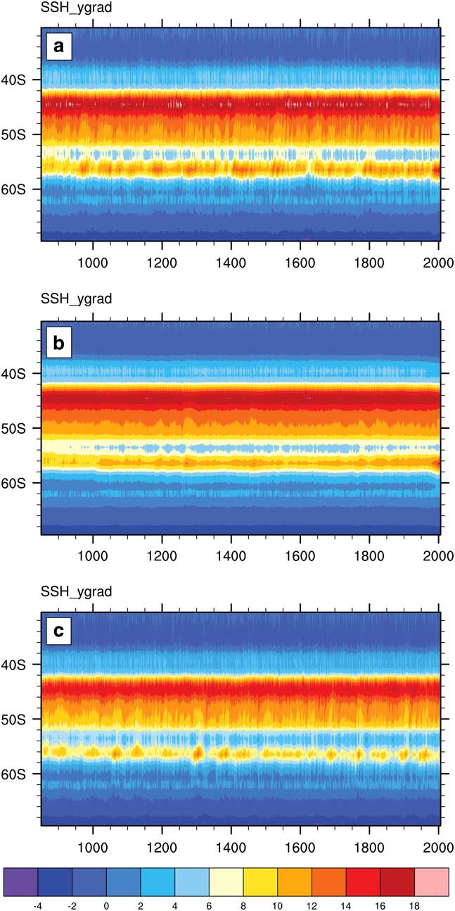
Fig. 2 The SSH gradient 0.01 cm km-1 between 30°S and 70°S in the western Atlantic (25°W) for a. ensemble member number 10, b. the ensemble average and, c. the 850 control simulation.
It is known that the positions of the Southern Ocean fronts are variable with longitude (Dong et al. Reference Dong, Sprintall and Gille2006, Sokolov & Rintoul Reference Sokolov and Rintoul2009, Kim & Orsi Reference Kim and Orsi2014). This paper examines their changes in the Southwestern Atlantic at 25◦W. This longitude was chosen because it is the location of a World Ocean Circulation Experiment (WOCE) section (A16) whose data is incorporated in the World Ocean Atlas 2013 version 2 (WOA13) product used for validation (Boyer et al. Reference Boyer, Antonov, Baranova, Coleman, Garcia and Grodsky2013).
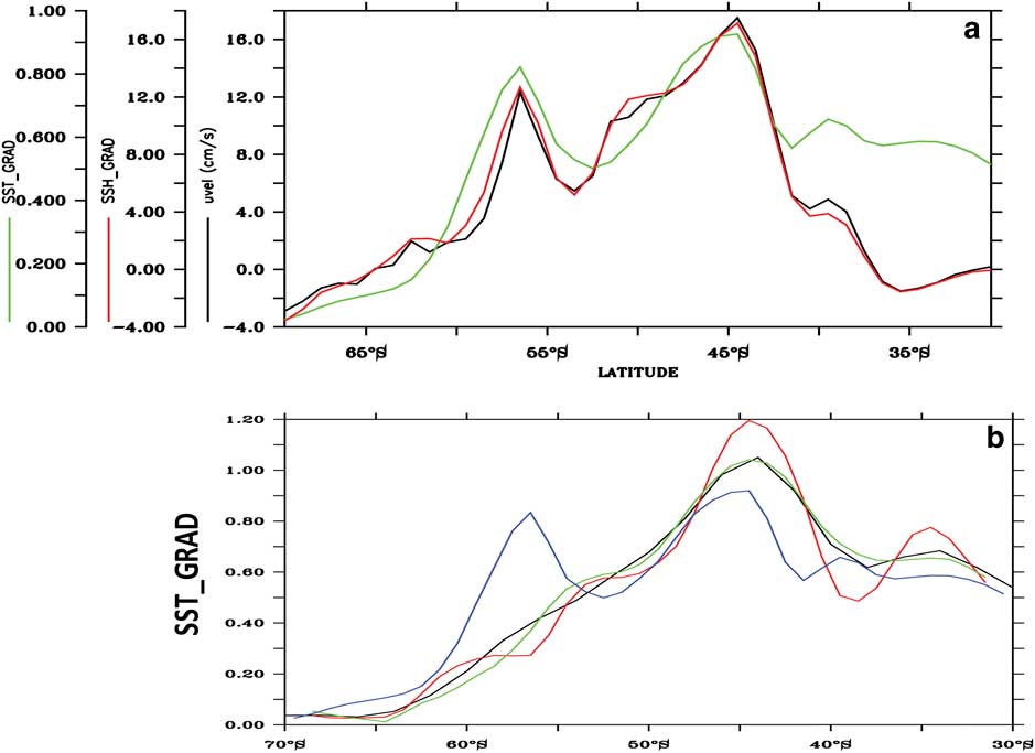
Figure 3a shows the ensemble mean for the period 1050–1950, of the SST gradient (green curve), SSH gradient (red curve) and the surface zonal velocity (black curve) as a function of latitude at 25°W. The maximum current speeds coincide with the maximum SSH and SST gradient values in the model, and are located at about 44°S and 56.5°S marking the locations of the SAF and PF respectively. Since SST gradients represent water mass boundaries, they can also indicate front locations (Dong et al. Reference Dong, Sprintall and Gille2006, Graham et al. Reference Graham, De Boer, Heywood, Chapman and Stevens2012). Figure 3b compares the front locations from SST gradients calculated using observations. The red curve is the SST gradient from NOAA-ERSST v4 (Huang et al. Reference Huang, Banzon, Freeman, Lawrimore, Liu and Peterson2015), the dark blue curve is from the WOA13 (Boyer et al. Reference Boyer, Antonov, Baranova, Coleman, Garcia and Grodsky2013), the light blue curve is from the Smith and Reynolds dataset (Smith & Reynolds Reference Smith and Reynolds2004) and the green curve is the SST gradient from the CESM-LME ensemble mean. When compared to observations, the location of the SAF in the model is in very good agreement while the magnitude of the model SST gradient is weaker (i.e. Fig. 3b). The PF is stronger in the model than in the observations, and the reason will be discussed below.

Fig. 3 a. The mean SSH gradient (0.01 cm km-1, red), SST gradient (0.01 °C km-1, green) and surface zonal velocity (cm s-1, black) at 25°W from the CESM-LME results. b. SST gradient from NOAA-ERSST (black); WOA13 (green); Reynolds and Smith (red); and the CESM-LME ensemble mean (blue).
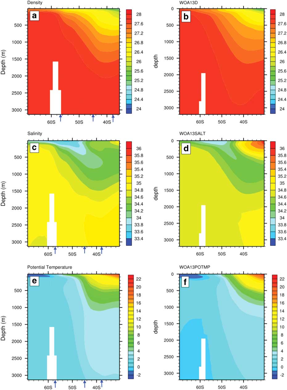
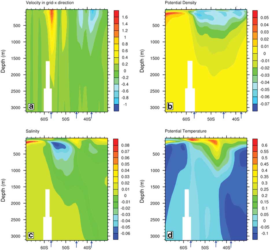
Figure 4 shows the mean vertical profiles of potential density (referenced to the surface, σθ), salinity and potential temperature for the period between 1970–2000 for the CESM (Fig. 4a, c & e) at 25°W between the latitudes of 30–70°S from the surface to 3000 m. These can be compared to the equivalent observed mean vertical profiles of density, salinity and temperature from the World Ocean Atlas 2013 (Fig. 4b, d & f, Boyer et al. (Reference Boyer, Antonov, Baranova, Coleman, Garcia and Grodsky2013)). In the absence of monthly (or annual mean) data from the WOA13 data product, the 1970–2000 mean, available for download at www.nodc.noaa.gov, was used for comparison with the model results.

Fig. 4 Mean vertical profiles at 25°W averaged for the period 1970–2000 from the model: a. potential density (σθ), c. salinity (psu) and e. potential temperature (°C). Compared with the mean vertical profiles at 25°W, averaged for the same period from the World Ocean Atlas 2013 b. potential density (WOA13D, σθ), d. salinity (WHOA13SALT, psu) and f. potential temperature (WHOA13POTMP, °C). The mean positions of the model STF (38°), SAF (44.6°) and PF (56.4°) are marked as blue arrows.
The vertical distribution of potential density for the model (referenced to the surface, σθ) in Fig. 4a and the density for WOA13 in Fig. 4b show upward tilts of the density surfaces that are quite similar. The model density is lower than the observations right at the surface between 52°S and 62°S, and is denser than WOA13 below 1500 m, north of 50°S by about 0.2 g cm-3. The salinity profiles from the model results and the WOA13 observations, presented in Fig. 4c and Fig. 4d respectively, exhibit the recognisable subsurface minimum signal associated with Antarctic Intermediate Water at about 55°S. The salinity minimum occupies the latitudes between the SAF and the PF. The salinity maximum located at the edge of the domain (c. 30°S) at the surface is associated with sub-Antarctic Mode Water (Talley, Reference Talley, Pickard, Emery and Swift2011).
The potential temperature field is well reproduced by the model (Fig. 4e) relative to the potential temperature field calculated from the WOA13 temperature (Fig. 4f). Mean profiles for both the CESM-LME and WOA13 show that in the southern part of the domain the water is coldest at the surface, where Antarctic Surface Water is located. However, the water column remains vertically stable because the lightest densities are at the surface where the water is very fresh because of melting sea ice. The smaller surface density between 52°S and 62°S is because the model is too warm right at the surface in this latitude band, which is primarily caused by the mixed layer depths being too shallow. South of 62°S the SST is in better agreement with WOA13, and this is the reason that the PF SST gradient at 56°S is much stronger in the model than in the observations (Fig. 3b). Below 1500 m, south of 55°S the model is 0.5–1 °C warmer than WOA13.
CESM results from the last millennium
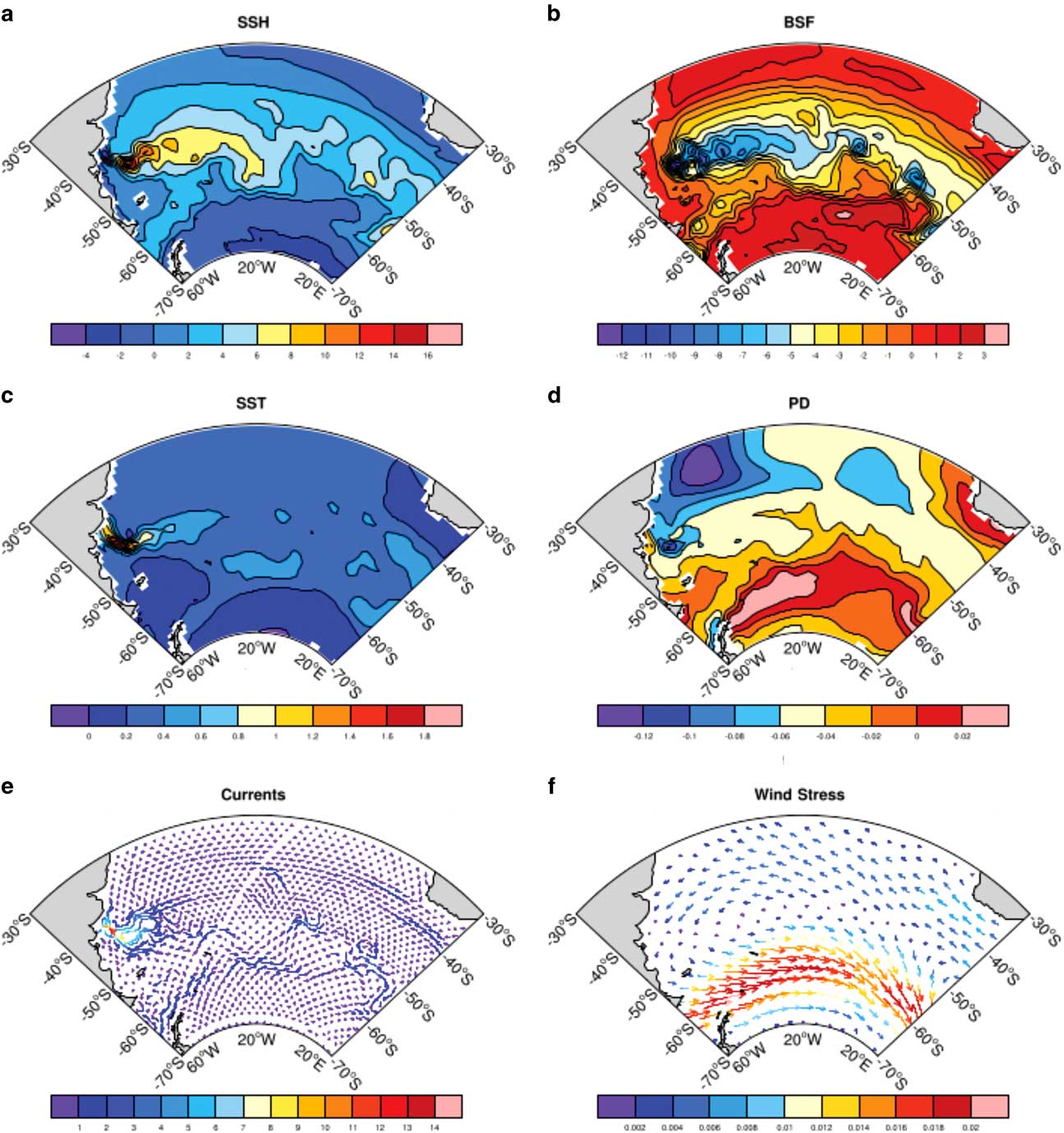
The spatial patterns averaged across 1050–1950 for SSH, barotropic streamfunction, SST, potential density (referenced to the surface, σθ), surface current and wind stress are shown in Fig. 5. The mean horizontal distribution of SSH and the barotropic streamfunction (Fig. 5a & b) show the subtropical and polar gyres that compose the upper circulation of the South Atlantic Ocean. They are represented by the positive SSH and anticyclonic circulation in the subtropics and negative SSH corresponding to the cyclonic subpolar circulation. This circulation pattern is described in detail in Stramma & England (Reference Stramma and England1999). The mean SST (Fig. 5c) shows that in the western Atlantic the colder Falkland Current waters reach northward to about 40°S next to the coast. The western subtropical Atlantic, north of 35°S has the warmest temperatures, around 22 °C. Warmer temperatures are also seen bordering the southern tip of Africa associated with the Agulhas Retroflection system. The latter is also the region with the lowest potential densities (Fig. 5d) around 1.023 g cm-3. Mean ocean surface current (Fig. 5e) and wind stress (Fig. 5f) are most intense in the ACC region between 40°S and 60°S. The Agulhas Retroflection, as well as the South Atlantic Current, which originates from the confluence of the southward flowing Brazil Current and the northward flowing Falkland Current, are noticeable features in the ocean surface current field, reaching speeds up to 60–65 cm s-1.
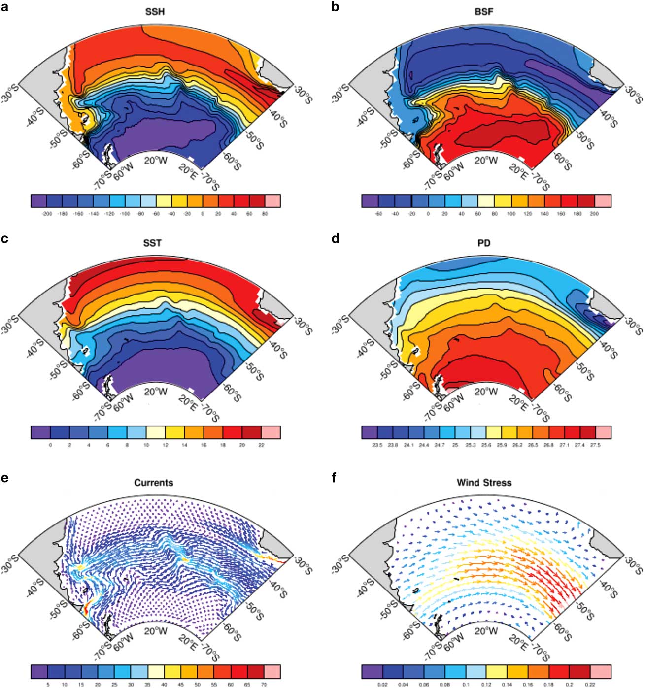
Fig. 5 Ensemble average mean for the 1050-1950 period: a. SSH (cm), b. barotropic streamfunction (Sv), c. SST (°C), d. sea surface potential density (σθ), e. surface current (cm s-1), f. wind stress (N m-2).
The band of westerlies is well marked in the wind-stress field (Fig. 5f) with maximum values east of 20°W. The westerlies decrease towards Antarctica and are associated with equatorward Ekman transport. North of the ACC region convergence in the Ekman transport implies downwelling, and south of the wind-stress maximum, divergence in the Ekman transport results in upwelling. This configuration causes a mean overturning circulation resulting in the isopycnals tilting upwards towards Antarctica.
The mean fields for the 1970–2000 period (not shown) are similar to those of the 1050–1950 period. However, there exist regional differences (Fig. 6) that reveal the degree of sensitivity of the South Atlantic when transitioning from the more stable 1050–1950 period into the greenhouse-gas driven late 20th century. The largest differences are spatially confined within the energetic Brazil–Falkland Confluence region near 40°S, next to the South American coast (Fig. 6a, b, c & e). The poleward shift of the Brazil Current results in a higher SST and SSH and stronger surface current near 45°S off the coast. This produces a reduction in the barotropic streamfunction in this region away from the coast. The mean difference in the wind stress between the 1050–1950 period and the last decades of the 20th century (1970–2000) shows a marked narrow band of westerly anomalies centred at 55°S where the increase in intensity of about 0.01 N m-2 is evident, as is the southward displacement of the maximum values. The increase in strength and southward displacement of the westerlies have been seen both in observations and in climate model results.

Fig. 6 Ensemble mean horizontal differences between the 1970–2000 mean and the 1050–1950 mean. a. SSH (cm), b. barotropic streamfunction (Sv), c. SST (°C), d. sea surface potential density (σθ), e. surface current (cm s-1), f. wind stress (N m-2).
Zonal wind stress
The westerly winds are not only important for the strength of the ACC, but they also drive northward Ekman transport in the region, which is associated with convergence to the north and divergence to the south of the maximum wind stress. The convergence/divergence pattern drives the vertical motions which are very important in setting up the ocean stratification and SSH gradients which are associated with the frontal positions. Changes in the winds are examined by looking first at the time series of changes in the latitude of the maximum annual zonal wind stress at 25°W, relative to its mean position over 1050–1950 (Fig. 7). The time series of the mean latitudinal position of the maximum zonal wind stress (maxTAUX) from 1050–1950 has virtually no trend. There are two episodes when the latitude of the maximum wind stress shifts abruptly almost 3° to the south. These coincide with volcanic eruptions at years 1258 and 1453, and are currently being explored in another study. The mean maxTAUX latitude for the 1050–1950 period is 51.5°S; for the 1970–2000 period it is a little to the south at 52.4°S. The standard deviation over 1050–1950 is 0.43°, so that the mean change over 1970–2000 of 0.9° is significant compared to the standard deviation.
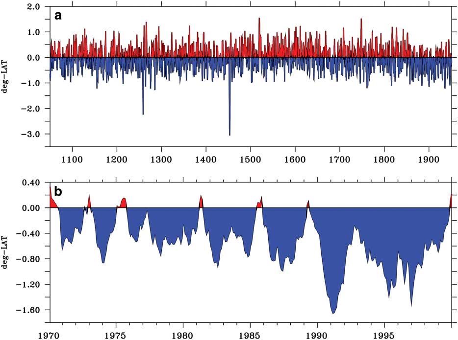
Fig. 7 Time series of the change in latitude of the maximum zonal wind stress about its mean position at 25°W. a. 1050–1950 period; b. 1970–2000 period. Note the different ordinate scaling between a and b.
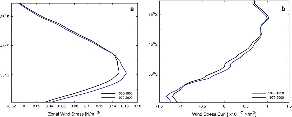
The zonally averaged zonal wind stress and wind-stress curl across the South Atlantic basin are shown in Fig. 8 for the 1050–1950 mean (black curve) and for the 1970–2000 mean (blue curve). The relative strengthening and poleward shift of the maximum zonal wind stress over the late 20th century is clearly seen between 50°S and 65°S (Fig. 8a). The maximum zonal wind stress increased by 0.01 N m-2 and moved nearly 1° to the south. The wind-stress curl (Fig. 8b) intensifies but does not shift its position. The changes shown in Fig. 8 lead to only a modest strengthening of the ACC with the mean transport through Drake Passage only increasing by 2.6 Sv in 1970–2000 over a mean transport of 160.5 Sv during 1050–1950.

Fig. 8 a. Zonal wind stress (N m-2) and b. wind-stress curl zonally averaged across the South Atlantic basin for the 1050–1950 period (black curve) and the 1970–2000 period (blue curve).
Figure 9 shows the time series of the transport between the southern limit of the ACC (62°S) and the location of the PF (56°S). There is low-frequency variability from 1050–1950 (Fig. 9a), with a standard deviation of 1.0 Sv. An increase in the transport between 56°S and 62°S starts in the 1970s, with less transport north of 56°S. The transport increase between 56°S and 62°S of 6 Sv is more than twice as large as the increase in ACC transport through Drake Passage. The small increase in ACC transport and southward shift, where an increase in zonal wind stress is imposed in the coupled model CCSM4, is known. Similar experiments and results have been documented in a range of other ocean and coupled models with horizontal resolution ranging from non-eddy-resolving to eddy-resolving.
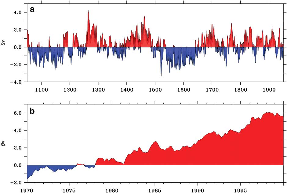
Fig. 9 Time series of the transport (Sv) between 62°S (southern limit of the ACC) and 56°S (the location of the PF) at 25°W. a. 1050–1950 period; b. 1970–2000 period. Note the different ordinate scaling between a and b.
The shift and intensification in the winds have an impact on the Southern Ocean sector of the South Atlantic. The differences in the mean profiles of zonal velocity, potential density (referenced to the surface, σθ), salinity and temperature between the 1970–2000 mean and the 1050–1950 mean are shown in Fig. 10. The zonal velocity in Fig. 10a shows intensification of the eastward velocities at 56°S, and that the maximum zonal velocity has shifted slightly to the south due to the small southward shift of the ACC.

Fig. 10 Ensemble mean vertical profile differences at 25°W between 1970–2000 mean and the 1050–1950 mean: a. surface zonal current (cm s-1), b. potential density (σθ), c. salinity (psu) and d. temperature (°C). The mean positions of the STF (38°), SAF (44.6°) and PF (56.4°) are marked as blue arrows.
Potential density differences (Fig. 10b) show that isopycnals deepen in the upper layers of the ACC region north of 60°S. The density increase south of 65°S between depths of 100–200 m is due to the salinity increase in the same region. The isopycnal slope change is consistent with a small southward movement of the ACC system. The salinity differences (Fig. 10c) are positive in the upper 200 m north of 50°S. The maximum salinity increase is between 60°S and 70°S in the upper 300 m.
The upper 200 m of the Southern Ocean has warmed (Fig. 10d) throughout the region. The largest subsurface warming occurs at 100 m depth with maximum values <0.7 °C, and the warming reaches down to 1000 m between 40°S and 50°S where surface water is subducted to form Antarctic Intermediate Water. The deeper ocean has cooled, and the cooling is strongest north of 40°S, below 2000 m. The warming right at the surface is relatively uniform between 30°S and 60°S, but there are subtle changes in the locations of the SAF and PF.
Changes in the frontal latitudes
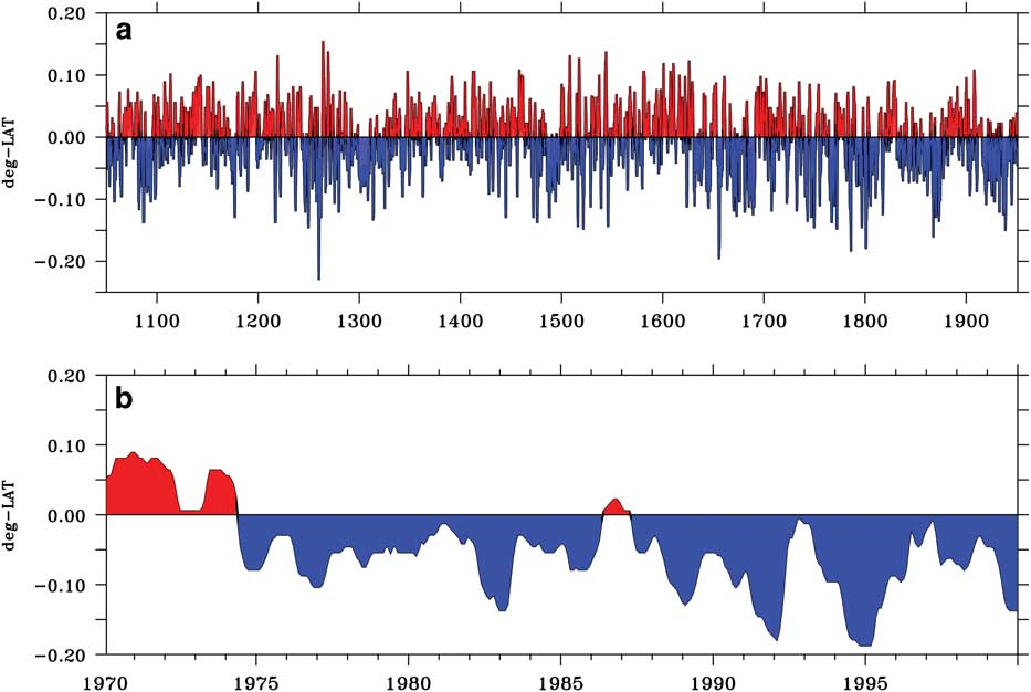
The time series of the SAF latitudinal position is obtained by locating the maximum SSH gradient position from the ensemble mean (Fig. 2b) between 40–50°S. The mean SAF position at 25°W over the years 1050–1950 is 44.6°S. Figure 11a shows the latitude with respect to the mean over 1050–1950, and Fig. 11b shows the latitude with respect to the same mean over 1970–2000. There is a slight shift to the south of c. 0.15° in 1970–2000, but this shift is not significant compared to the standard deviation variation in latitude of 0.17° calculated from the 1050–1950 time series.

Fig. 11 Time series of the change in latitude of the SAF about its mean position obtained by locating the maximum SSH gradient position for the ensemble mean at 25°W between 40°S–50°S. a. 1050–1950 period; b. 1970–2000 period. Note the different ordinate scaling between a and b.
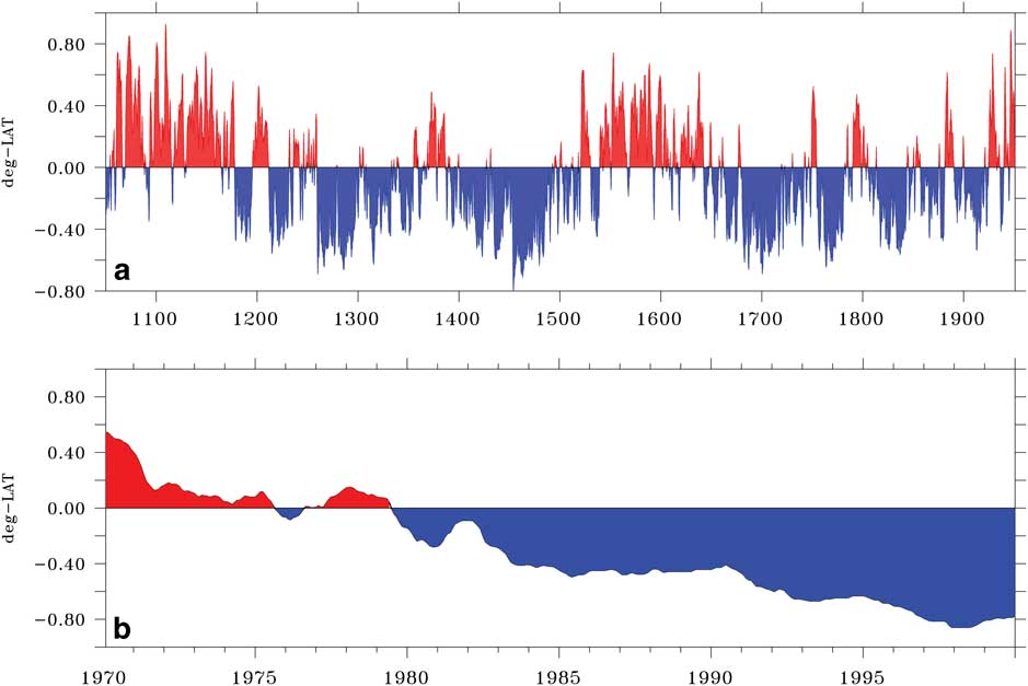
Figure 12 shows similar time series to Fig. 11 except for the PF, which has a mean latitude of 56.4°S over 1050–1950. Figure 12b shows that the PF has moved about 0.8° to the south in 1970–2000, and this is a significant shift compared to the standard deviation of 0.33° latitude calculated from the 1050–1950 time series. Kim & Orsi (Reference Kim and Orsi2014) use SSH altimetry data from 1992–2011 to compute the variability of ACC frontal positions in a similar way, by subtracting the mean latitude from their time series of latitudinal position for each front. However, unlike this study, they zonally average their results. Their Fig. 8 shows that the analysed fronts (SAF, PF, and the Southern ACC Front) have moved poleward, but the shifts are very small. In agreement with the results presented here, they show an increased southward displacement with higher latitude, which means that the southernmost fronts (Southern ACC Front in their case) experienced the largest southward shift within the analysed period.

Fig. 12 Time series of the change in latitude of the PF about its mean position obtained by locating the maximum SSH gradient position for the ensemble mean at 25°W between 50°S–60°S. a. 1050–1950 period; b. set1970–2000 period. Note the different ordinate scaling between a and b. The PF has moved about 0.8° to the south in 1970–2000; this is a significant shift compared to the standard deviation of 0.33° latitude calculated from the 1050–1950 time series.
The changes in latitude of the PF are strongly negatively correlated to the transport between 56◦S and 62◦S shown in Fig. 9. Between the years 1050–1200, the PF is displaced northward and the transport is reduced. In contrast, for the years 1200–1500 the PF is displaced southwards and the transport is increased, and the phase changes again over the years 1500–1650. Therefore, the PF changes its latitude due to small movements north and south of the core position of the ACC. Figure 9b shows that the ACC moves to the south between 1970–2000 with increased transport between 56°S and 62°S. A consequence of the ACC moving southwards is that the PF is displaced to the south by 0.8° in 1970–2000. Both of these shifts stand out compared to the model standard deviation over the years 1050–1950. Similar southward shifts of the South Atlantic fronts and the ACC transport between them have been seen previously in the data from GFDL CM2.1 (a global coupled climate model developed at the Geophysical Fluid Dynamics Lab (GFDL) of the National Oceanic and Atmospheric Administration (Delworth et al. Reference Delworth, Broccoli, Rosati, Stouffer, Balaji and Beesley2006), version 2.1).
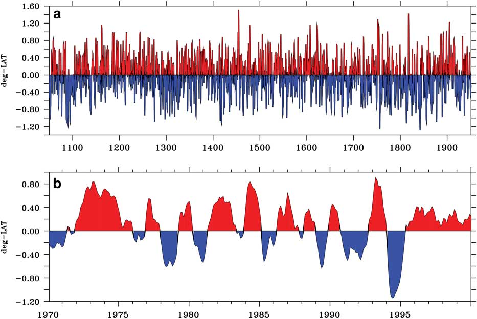
Although the Subtropical Front (STF), which is located between 30–40°S, is not clearly identified as a maximum in the SSH gradient (Fig. 2), examination of the SST gradient at 25°W reveals its location in all CESM-LME ensemble members. The STF is characterized as a surface discontinuity in temperature which begins in the west in the Brazil–Falkland Confluence region, and reaches east towards South Africa. According to Smythe-Wright et al. (Reference Smythe-Wright, Chapman, Duncombe Rae, Shannon and Boswell1998) the latitudinal position of the STF is about 38°S in the western Atlantic, which is similar to the CESM-LME location. The changes of the STF location at 25°W about the 1050–1950 mean of 37.3°S for both 1050–1950 and 1970–2000 are shown in Fig. 13. There is almost no change in the mean latitude near the end of the 20th century compared to the standard deviation over 1050–1950. This lack of trend is consistent with the very small changes in the zonal wind-stress curl between 30°S and 40°S at the end of the 20th century shown in Fig. 8b.

Fig. 13 Time series of the change in latitude of the STF about its mean position obtained by locating the maximum SST gradient position for the ensemble mean at 25°W between 30°S–40°S. a. 1050–1950 period, b. 1970–2000 period. Note the different ordinate scaling between a and b.
Polar Front at other longitudes
Most of the results shown so far are from longitude 25°W, but Fig. 6 shows that the changes late in the 20th century are not zonally uniform. The dynamics of the South Atlantic are not longitudinally homogeneous: the southwest is influenced by an extended continental shelf, the central basin is influenced by the mid-Atlantic ridge, and the southeast is impacted by effects from the Agulhas retroflection. Figure 14 shows the time series of the PF latitude over the period 1970–2000 relative to its 1050–1950 mean at longitudes 45°W, 0°E and 10°E. Comparison with Fig. 12b at 25°W shows that there is very little change in latitude at 45°W and 0°E. The PF does move a little to the south at 10°E after 1985, but the change is small compared to the southward shift at 25°W. None of the changes at other longitudes are significant by comparison with the standard deviation over 1050–1950. This result agrees with Fig. 8 of Kim & Orsi (Reference Kim and Orsi2014), which shows that the largest southward shift of the PF in the South Atlantic over 1993–2010 occurs near 25°W. Furthermore, recent results suggest that the PF further east in the Atlantic is far from the latitude of maximum westerlies and their southward displacement. The same study shows that the STF near Africa responds to the dynamics of both the Indian and Atlantic subtropical gyres. Therefore, the position of the PF at other longitudes could be responding to the dynamics of the subtropical gyre and only indirectly linked to the local winds.
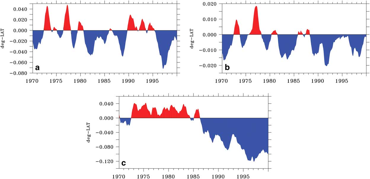
Fig. 14 Time series of the change in latitude of the PF over 1970–2000 relative to its 1050–1950 mean at a. 45°W, b. 0°E and c. 10°E.
Figure 15 shows the time series of the maximum SSH gradient between 50°S and 60°S over 1970–2000 at the four different longitudes. It shows that the SSH gradient associated with the PF increases over this period at all four longitudes. However, the increase is much larger at 25°W, where it increases from 0.11 cm km-1 in 1970 to 0.15 cm km-1 in 2000. The increases at the other longitudes over this period are all less than 10%.
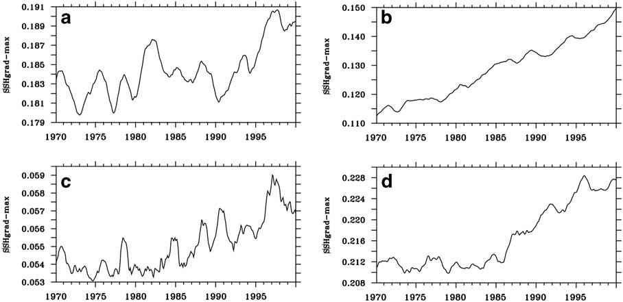
Fig. 15 Time series of the maximum SSH gradient (cm km-1) between 50°S–60°S for a. 45°W, b. 25°W, c. 0°E and, d. 10°E.
Summary and conclusions
This study has focused on the ACC system changes associated with the sub-Antarctic Front (SAF) and Polar Front (PF) zones, since it is where most of the ACC transport is carried. The STF, to the north of the SAF, was also analysed because it represents the boundary between the ACC region and the subtropical gyre. The purpose was to characterize the mean climatology of the relevant ocean fields with emphasis on late 20th century changes (1970–2000) relative to the period 1050–1950. The ACC fronts were identified through the maximum values in SSH and SST gradients in all ten CESM-LME ensemble members. Since the position of the Southern Ocean fronts at 25°W were consistent in all members, the ensemble average results were used to characterize the forced anthropogenic response during 1970–2000, compared to the much more weakly forced period of 1050–1950.
Temperature, salinity and density profiles at 25°W from the ensemble mean simulation were compared in Fig. 4 with the equivalent data from the World Ocean Atlas 2013, which showed that the model and WOA13 profiles are quite similar. It was found that the major differences between the means of the 1050–1950 period and the late 20th century (1970–2000) are located in the ACC region between 40–60°S including the Brazil–Falkland confluence region. Analysed fields were SSH, barotropic streamfunction, SST, potential density, surface current and wind stress.
The water column down to 3000 m (Fig. 10) showed significant differences over depth between the 1050–1950 period and the 1970–2000 period, most pronounced in the ACC region marking the location of the PF and SAF. In the late 20th century (1970–2000) there is freshening of Antarctic Intermediate Water but, in contrast, Circumpolar Deep Water becomes saltier. Further north the subsurface sub-Antarctic Mode Water freshens and warms slightly.
Considering the significance of the SAF and PF for the ACC system, their time series were analysed for the South Atlantic at 25°W. An index for the variability of their position was obtained by using the latitude of the maximum SSH gradient (PF and SAF) between 40–60°S. An index for the STF between 30–40°S was also obtained using the maximum SST gradient.
Results show that there is low-frequency variability in the position of the fronts in both periods (i.e. 1050–1950 and 1970–2000) with changes between the two periods that can be related to the change in the model wind stress. The changes in the frontal positions can be summarized (from south to north) as follows. The PF shows a southward shift starting in the 1970s that is significant compared to variability over 1050–1950. There is a small southward trend in the SAF position after the 1980s, but it is not significant compared to the 1050–1950 variability. Both are responding to wind changes, which also reveal a clear southward trend starting in the 1970s. Further north, the STF shows no trend in its mean position because there is very little change in the zonal wind stress between 30–40°S (Fig. 8). Results from other longitudes show that changes in the PF latitude and strength are considerably smaller than the changes at 25°W.
These CESM-LME results are consistent with the idea that the ACC transport is not very sensitive to changes in the wind-stress forcing. The average CESM-LME transport through Drake Passage over 1970–2000 is only 2.6 Sv larger than the 1050–1950 mean of 160.5 Sv. This increase is double the standard deviation of the transport during 1050–1950, which is 1.3 Sv. The degree of eddy saturation and compensation in the CESM with a non-eddy-resolving ocean component is similar to results from eddy-resolving models.
Acknowledgements
This study was supported by grant FAPESP 2015/17659-0 and grants CNPq-301726/2013-2; CNPq-405869/2013-4; CNPq-MCT-INCT-594-CRIO; 573720/2008-8; Coordenação de Aperfeiçoamento de Pessoal de Nível Superior - Brasil (CAPES) - Finance Code 001. IW thanks Bette Otto-Bliesner from the National Center for Atmospheric Research (NCAR) for making the CESM-LME data available and Martim Mas for help with schematics. The authors also wish to thank two anonymous reviewers for their helpful comments and suggestions. Monthly, daily and six-hourly outputs are saved and archived on the Earth System Grid (http://www.earthsystemgrid.org) as single variable time series. NCAR is funded by the National Science Foundation.
Data deposit
The data used in this study is readily available for download from the Climate Data Gateway at NCAR at www.earthsystemgrid.org
Author contribution statement
Both authors conceived the presented idea. I.W. developed the idea further and performed the computations and plots. P.G. verified the statistics. Both authors discussed the results and contributed to the final manuscript.