Nomenclature

C _p

pressure coefficient (p–p _∞) / (½ρU ²)

H

total head (p–p _∞+ ½ρu ² )/ (½ρU ²)

L

root chord

p

pressure

p _∞

upstream pressure

Q

normalised 2nd invariant of the velocity tensor

Re

Reynolds number ρUL/μ

Re_r

Reynolds number based on local wing semi-span

s

wing semi-span

u

local flow speed

U

upstream flow speed

x,y,z

spatial coordinates

α

angle of incidence

γ

semi-apex angle

μ

dynamic viscosity

ρ

density

2.0 NUMERICAL METHODS

The numerical results presented here have been obtained using the ANSYS CFX software, a commercial CFD package. Full details on the software can be found in the program documentation^{( 14 )}. Only brief details are, therefore, presented here. The software uses a conservative control volume finite element method, using a cell-vertex formulation for constructing the discrete equations. These discrete equations are solved with a coupled equation solver using the Algebraic Multi-Grid Method, which typically gives good convergence characteristics, see Raw⁽ Reference Raw ^{15 )}. A modified version of the Rhie and Chow algorithm⁽ Reference Rhie and Chow ^{16 )} is used to prevent oscillations associated with the use of central differencing for the pressure gradient terms. For the results presented in this paper, the flow is assumed to be an incompressible laminar flow with constant viscosity. Default discretisations have been used, with a high-resolution blended differencing scheme for advective terms, and central differencing for diffusion terms. These are generally second-order accurate, except when local cell Reynolds numbers are high when the results are blended with a first-order method to avoid overshoots in the solution. In the limit of the mesh size tending to zero, these methods are formally second-order accurate.

3.0 GEOMETRY AND MESH GENERATION

The flow geometry is a delta wing of semi-apex angle γ enclosed in a rectangular domain whose walls are sufficiently far enough away so as not to influence the results. As the geometry is symmetric in the cases studied here, the symmetry has been exploited in the model to reduce the number of grid points required. A triangular cross-section consistent with the finite thickness of the wings in the experiments was used for the model of the delta wings. The wing is perpendicular to the inlet face of the domain, with the x-axis in the plane of the delta wing, the y-axis vertically up and the z-axis along the delta wing. To achieve the desired angle of incidence the flow is inclined at an angle α upwards at the inflow face. This is illustrated in Fig. 1.

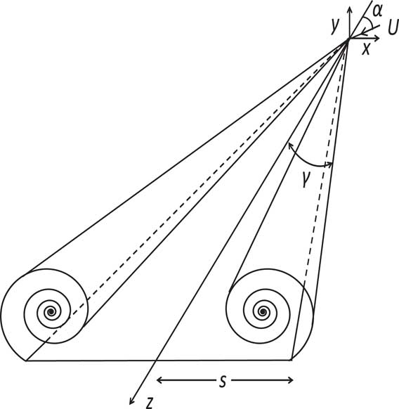
Figure 1 Schematic representation of leading edge vortices.

Unstructured mixed element meshes were used, with prismatic wedge elements near the solid wing surface, and tetrahedral elements in the bulk of the flow. Mesh controls were used to refine the mesh close to the wing surface and in the region where the vortex sheet and vortex core were expected. A prismatic mesh was used near the solid surfaces, to get good boundary layer resolution, following the recommendations of ERCOFTAC’s best practice guidelines^{( 17 )}.

This problem is characterised by a high Reynolds number for laminar flows, leading to large variations in length scales, from the larger scales of the overall geometry to the very thin laminar boundary layers and vortex sheets. It is unlikely therefore that the mesh can resolve everything in the flow, particularly towards the trailing edge of the wing where the flow in the vortex cores and in the boundary layer undergo a transition to turbulence. However, the meshes used in this study should be adequate to look at the overall flow structure upstream of the trailing edge, and to establish the trends as the relevant parameters are varied. The studies have been repeated with many different meshes employing varying numbers of grid points and mesh distributions. Provided sufficient resolution is used in the boundary layers and near the leading edge, the results from these meshes are very similar to those presented here, which have used the largest number of mesh cells, with points concentrated in key regions.

It is not easy to get suitable mesh resolution in the neighbourhood of the vortex sheet and core with manual mesh generation, as the location of these flow structures is not known a priori. The software has an adaptive meshing capability, increasing the mesh density based on gradients of a solution variable. Vorticity magnitude is often used as the reference variable on which to adapt, but in the present case the vorticity variations generated in the boundary layer and near the trailing edge will be greater than that in the vortex sheet, and hence the mesh can be over-refined in the boundary layer. A number of different indicator variables were tested to increase resolution in the vortex sheet and core. For the results presented here, the variation of the total pressure was used as the adaption variable. This concentrated the mesh near to the leading edge of the wing to capture the sharp gradients in the primary variables in this region, although it did not concentrate the mesh significantly near the vortex sheets as the total pressure is comparatively smooth across a vortex sheet.

Information on the mesh sizes used for each case is provided later, and further detailed information on the geometries and meshes, including a mesh sensitivity study, is contained in the Supplementary information⁽ Reference Jones and Riley ^{13 )}.

4.0 CASE STUDIES OVERVIEW

This paper focuses mainly on two geometrical configurations for which quantitative experimental information on the secondary flow structures is available:

1. 1. The experiments of Fink and Taylor⁽ Reference Fink and Taylor ^{18 )}. Comparisons have been carried out with the surface pressures on the wing surface, for which theoretical results are available from vortex sheet methods, and from the hybrid method of Kirkkopru and Riley⁽ Reference Kirkkopru and Riley ^{10 )}. Fink and Taylor also present results for the total head, which are compared with the CFD results.

2. 2. The measurements of Marsden, Simpson and Rainbird⁽ Reference Marsden, Simpson and Rainbird ^{19 )} on a delta wing with a larger apex angle. Again, contours of the total head are available, along with pressure coefficients on the wing surface.

The paper also discusses qualitative comparisons with other available data for slender delta wings.

Table 1 gives some of the main parameters for the cases considered here. It should be noted that the Reynolds numbers for these cases are high for laminar flow conditions and the flow can be expected to be turbulent in places, particularly near to the trailing edge. This can make convergence of the iterative procedure difficult to achieve. The convergence of the results is described briefly later and in more detail in the Supplementary information⁽ Reference Jones and Riley ^{13 )}.

Table 1 Geometric and flow parameters: experimental data

5.0 FINK AND TAYLOR

5.1 Geometricalconfigurationsandmesh

Fink and Taylor⁽ Reference Fink and Taylor ^{18 )} carried out studies for two slightly different delta wings. Wing E1 was made from a flat plate 0.128 in. thick, with a constant chamfer of 0.75 in. on both sides parallel to the leading edges. Because of a concern that the chamfer might induce a secondary flow separation, the second wing E2 had the same plan form, thickness and material as E1, but with a flat suction surface and a longer chamfer of 1.5 in. parallel to the leading edge. As their total head traverses were reported for wing E2, the geometry used for the CFD was similar to wing E2, with a flat suction surface aligned with the x-axis.

The meshes used were generated using the meshing procedure outlined earlier and the mesh sizes used are given in Table 2.

Table 2 Mesh sizes, Fink and Taylor configuration

5.2 Results:totalheadcontours

Figures 2, 3 and 4 show the total head, H, on the measuring section, 0.417 of root chord, for both the computations and the measurements on wing E2 for α=5°, 10° and 15°, respectively. The total head is defined by

$$H{\equals}(p{\rm }{\minus}{\rm }p_{\infty} {\plus}{\rm }\raise.5ex\hbox{$\scriptstyle 1$}\kern-.1em/ \kern-.15em\lower.25ex\hbox{$\scriptstyle 2$} {\rm \rho }u^{2} )\,/\,{\rm }($\scriptstyle \raise.5ex1$}\kern-.1em/ \kern-.15em\lower.25ex\hbox{$\scriptstyle 2$} {\rm \rho }U^{2} ),$$

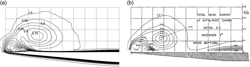
Figure 2 Total head contours, α=5º, (a) CFD and (b) measurements from Fink and Taylor.

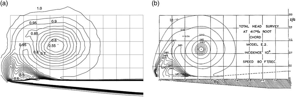
Figure 3 Total head contours, α=10º, (a) CFD and (b) measurements from Fink and Taylor.

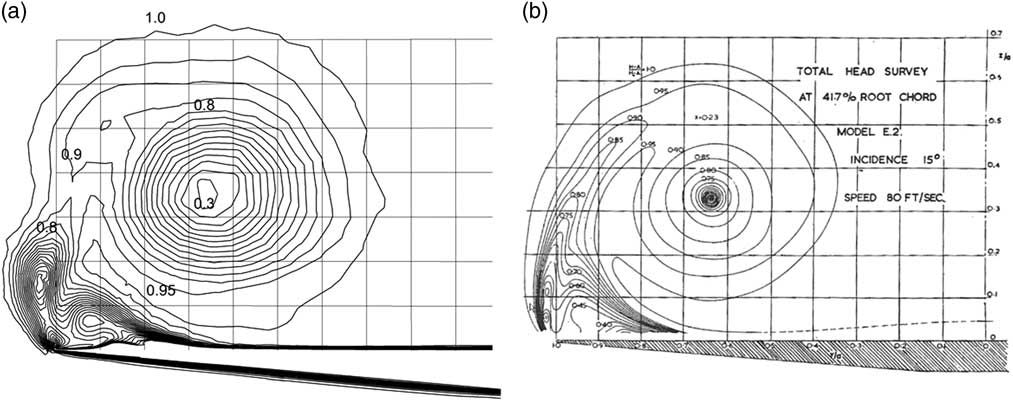
Figure 4 Total head contours, α=15º, (a) CFD and (b) measurements from Fink and Taylor.

where p is the pressure, p _∞ the upstream pressure, ρ the density, u the local flow speed and U the upstream speed. While the contours of H are not streamlines in a 3D viscous flow, they do give a good idea of the major recirculating flow structures in the cross-flow plane.

The graticules in the figures are at 10% of local wing semi-span in both the measurement and computational results. The very small differences between the triangular cross-section in the model and that of wing E2 can be seen in Figs 2(a) and (b). These differences should not materially affect the comparison.

The computations predict very well the overall flow structure in the measurement section. This includes the size and location of the primary vortex, as well as the main characteristics of the secondary flow near to the wing tip. Furthermore, the values of the contour lines of total head H are in good agreement, and show more intense primary vortices as the angle of incidence is increased. The details of the secondary flows are not quite as well represented, although there are very strong similarities between them. For example, for an incidence of 5° in Fig. 2(b) the measurements show a thickening boundary layer which might not have separated, whereas the simulations in Fig. 2(a) indicate clearly defined secondary separated flows, with two small flow structures, one associated with a secondary separation induced by the primary vortex at 90% of the semi-span, and a second one close to the leading edge. The location of the vortex centre and the values of H within the main vortex are in good agreement with a minimum value of around 0.75. For α=10° in Fig. 3, there are well-developed secondary recirculations in both the computations and the measurements, with the one at the leading edge becoming more elongated and aligned with the vortex sheet. At α=15°, the recirculation at the leading edge has become more elongated and has sub-divided in two. This structure is more pronounced in the simulations but is clearly apparent in the measurements. It will be seen later that the detailed flow structure of this recirculation changes considerably over a small downstream distance, and hence the details will be sensitive to the location of the cross-section.

The secondary vortex beneath the primary vortex has also moved closer to the leading edge with increasing α, to around 95% of the wing semi-span for α=15°. In the simulations, the contours beneath these secondary vortex sheets in the boundary layer have developed bumps, indicating a thickening of the boundary layer in these regions. The implications of these results for the 3D flow structures are discussed in more detail later in Section 7 of this paper.

Lowson⁽ Reference Lowson ^{20 )} obtained results for the shape of the vortex sheet from smoke visualisations and compared his results with Fink and Taylor’s total head contours for α/γ=1.0 and 1.5 shown in Figs 3(b) and 4(b), using the values of 0.95 and 1.0 to represent the vortex sheet shape. He noted ‘the close agreement in the shape of the feeding sheet between the present low-speed visualisations and the total head surveys at higher Re is noteworthy’. Given the close agreement between the total head surveys and the current CFD results in Figs 3 and 4, we can infer that the predicted vortex sheet shapes are also in close agreement with Lowson’s visualisations for the sheet shape, even though the inflow speeds are different.

5.3 Results:pressurecoefficients

Figure 5 shows the pressure coefficients Cp=(p–p _∞)/(1/2ρU ²) on the wing at the measuring section from the CFD from wing E2 and the measurements at α=15º for wings E2, and wing E1 for α=5º and 10º for both the left- and right-hand sides of the wing. The agreement is remarkably good for all three angles of incidence. Fink and Taylor noted a stronger secondary separation for Wing E1 and an increased extent for the constant pressure region outboard of the suction peaks for wing E2, but ‘in other respects the results were quite comparable with those on wing E1’. Fink and Taylor⁽ Reference Fink and Taylor ^{18 )} did also give the pressure coefficient for both wing E1 and E2 at α=15º. A comparison between the results for the two wings shows the differences in Cp are relatively small.

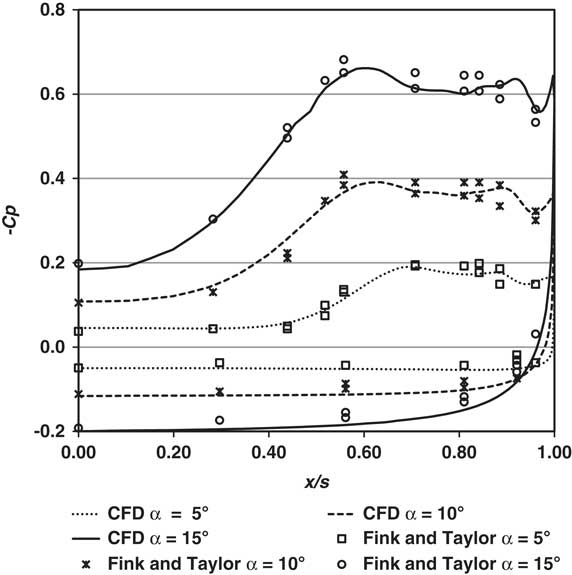
Figure 5 Pressure coefficients, -Cp on the upper and the lower wing surface for different angles of incidence.

5.4 Comparisonwithvortexsheetmethods

Having demonstrated earlier that the computations compare well with the measurements, this section compares the computations with previous results for vortex sheet methods, especially the original inviscid results of Smith and others⁽ Reference Smith ^{5 –} Reference Barsby ^{7 )} and the combined vortex-sheet and boundary-layer method of Kirkkopru and Riley⁽ Reference Kirkkopru and Riley ^{10 )}, which takes the finite thickness of the boundary layer and vortex sheet into account. The results presented in⁽ Reference Kirkkopru and Riley ^{10 )} were for α=10° at a Reynolds number Re_r=5.0E04 based on the local wing semi-span. However, Kirkkopru and Riley⁽ Reference Kirkkopru and Riley ^{10 )} did note that their results for the pressure distribution were relatively insensitive to the Reynolds number.

Figure 6 shows a comparison of results for the pressure coefficient, Cp, for α=10º between the inviscid results of Smith⁽ Reference Smith ^{5 )}, the current CFD approach, the measurements of Fink and Taylor, and the calculations of Kirkkopru and Riley⁽ Reference Kirkkopru and Riley ^{10 )}. In order to mimic the effects of an inviscid flow, an additional CFD calculation was carried out by applying a ‘free-slip’ zero shear stress boundary condition on the delta wing, instead of a no-slip condition. With this condition, secondary separation on the wing surface does not take place. The rest of the set-up was identical to that for the results for the no-slip condition presented here. The comparison indicates:

• ∙ For the ‘inviscid’ CFD with the zero shear stress boundary condition, the results are close to those of Smith, with a comparable value for the peak suction, but with a slightly broader peak, giving increased confidence in the CFD methodology and also in the accuracy of the vortex-sheet methods for the inviscid flow. Further results from the ‘inviscid’ CFD model are given in the Supplementary information⁽ Reference Jones and Riley ^{13 )}.

• ∙ The results from the inviscid-viscous coupling method of Kirkkopru and Riley⁽ Reference Kirkkopru and Riley ^{10 )} are in qualitative agreement with the CFD and the experiments, with a significant flattening of the suction peak, compared with those of Smith, in accordance with the development of a thick boundary layer, and the resulting secondary separation. The peak values are, however, somewhat less than those of Fink and Taylor⁽ Reference Fink and Taylor ^{18 )}.

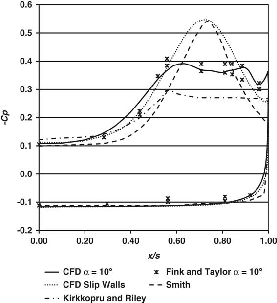
Figure 6 Pressure coefficients, -Cp on the upper and the lower wing surface, α=10°.

From the general agreement in the structure of these plots with the overall trend of the broadening of the peak, and reduction of the peak suction from the inviscid models, we concur with the conclusion of Kirkkopru and Riley⁽ Reference Kirkkopru and Riley ^{10 )} that ‘the main effect which controls the overall flow properties is the separation and displacement effect on the wing surface’ rather than the specific details of the separated viscous flow. This is corroborated by the results from the next section where the flow structure from a wing with larger apex angle is considered.

6.0 MARSDEN, SIMPSON AND RAINBIRD

Marsden, Simpson and Rainbird⁽ Reference Marsden, Simpson and Rainbird ^{19 )} carried out measurements on two different delta wings. The one studied here is their Model II wing, for which they made detailed measurements. This wing has a 40° apex angle, double that of Fink and Taylor, with a higher inlet flow speed, 130 ft/s. As a result, the Reynolds number based on wing semi-span is greater than that of Fink and Taylor. A laminar CFD flow model at 130 ft/s failed to converge, exhibiting large fluctuations in the flow, and significant grid dependence. As a result, these results were not felt to be reliable. To gain some insight into the nature of the flow, calculations were carried out at a flow rate 1/10 of that in the measurements, 13 ft/s, a Reynolds number of 1.2E5. These results were then compared with normalised data. These comparisons showed very interesting correlations with the measurements, and, for this reason, they are discussed below.

These results did not fully converge exhibiting larger residuals at the trailing edge and small fluctuations in values of the variables near the trailing edge and downstream of the trailing edge. For a strongly convective flow such as this, we can expect that these fluctuations have little impact on values upstream. To confirm this, for the most difficult case with α=14.0°, during the iterations, results at representative monitor points were sampled, and the results upstream of the most downstream measurement station, Station 1 at 83% of root chord, were steady, and the residuals upstream of this station were all small. Detailed information on the convergence behaviour is provided in the Supplementary information⁽ Reference Jones and Riley ^{13 )}.

The mesh sizes are given in Table 3. An adaptive mesh was used initially at α=8.8°. The same mesh was used for α=14.0°.

Table 3 Mesh sizes, Marsden, Simpson and Rainbird configuration

CFD results are presented here for two angles of incidence, 8.8° and 14.0°, for which surface Cp values were presented at four measurement stations, at 83%, 67%, 50% and 33% of root chord, respectively, with Station 1 being closest to the trailing edge. Marsden et al.⁽ Reference Marsden, Simpson and Rainbird ^{19 )} presented surface Cp results for higher angles of incidence, but for these cases, the CFD results indicated significant unsteady effects emanating from the trailing edge, and so they are not considered here.

Figure 7(a–d) plots the pressure coefficient values at the four measuring stations for α=8.8°. The measurement traverses were carried out across the whole of the wing surface, and because of the geometrical symmetry, the data from both sides of the wing are included in the diagrams, to give an indication of the scatter in the data.

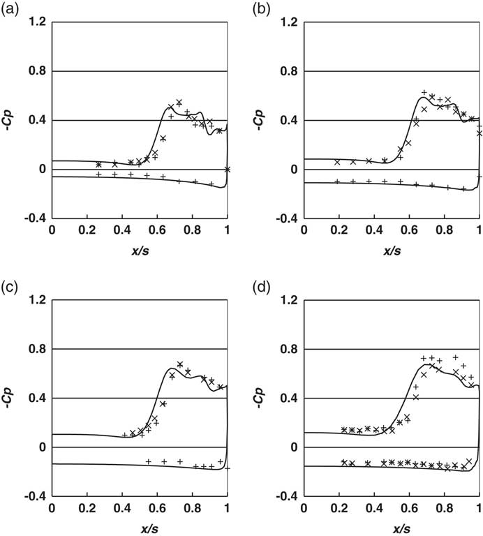
Figure 7 -Cp vs. x/s, α=8.8°, CFD ───, data right side +, data left side ×, (a) Station 1, (b) Station 2, (c) Station 3 and (d) Station 4.

The simulations show very good agreement with the measured data, reproducing the values and overall trends in the results very well, with a broad suction peak in both the measurements and the computations. The results also show the peak suction reducing in the direction of the trailing edge, from Stations 4 to 1, indicating that the flow is not conical.

Figure 8(a–d) plots the same data for α=14°. Again, the agreement is good, with similar trends in the results.

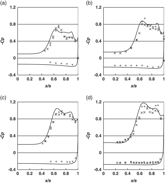
Figure 8 -Cp vs. x/s, α=14°, CFD ───, data right side +, data left side ×, (a) Station 1, (b) Station 2, (c) Station 3 and (d) Station 4.

It is difficult to infer the overall flow structure, especially the details of any secondary flows from these surface traverses. In addition to the pressure coefficients on the wing surface, Marsden et al.⁽ Reference Marsden, Simpson and Rainbird ^{19 )} also carried out a traverse measuring the total head at just one location, Station 2 for α=3.9°, 8.8° and 14.0°. For α=3.9°, the boundary layer was attached, and no secondary flow structures were visible in their plots. For this reason, they are not considered here.

Figure 9(a) and (b) shows the contours of the total head for α=8.8° from the CFD and the equivalent contours presented by Marsden et al⁽ Reference Marsden, Simpson and Rainbird ^{19 )}. Figure 10(a) and (b) shows the same information for α=14°. The graticules shown are at intervals of 10% of the wing semi-span in both the measurements and the computations. The locations of the primary vortex centre are very well predicted, and the sizes of the primary vortices are similar. Both the computations and the measurements show complex secondary flow structures close to the leading edge, consistent with the presence of secondary and tertiary vortices. It should be noted that the probe size in the measurements was 0.2 in., about half the distance between the graticules in Fig. 10(a). Marsden et al.⁽ Reference Marsden, Simpson and Rainbird ^{19 )} did comment that ‘the probe used was rather large and may influence the contours obtained’. This might make it difficult to get an accurate representation of the complex flow near the leading edge. Nevertheless, the general agreement in the flow characteristics and contour values for both angles of incidence is very encouraging, especially given the differences in the values of the Reynolds numbers.

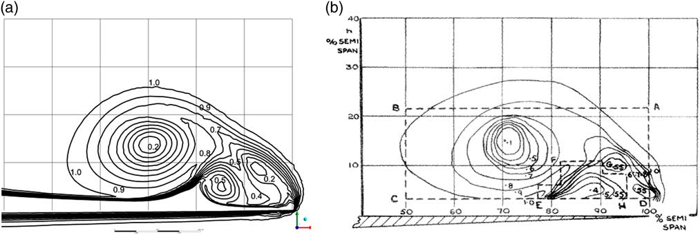
Figure 9 Total head contours, Station 2, α=8.8º, (a) CFD, (b) measurements, from Marsden, Simpson and Rainbird.

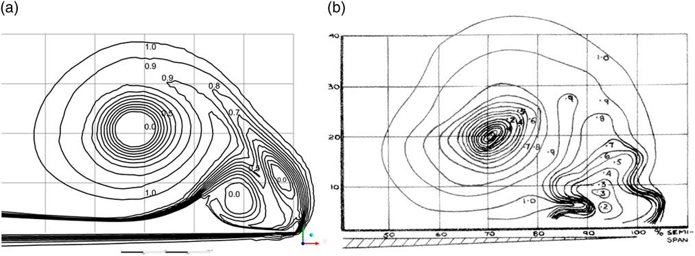
Figure 10 Total head contours, Station 2, α=14º, (a) CFD, (b) masurements, from Marsden, Simpson and Rainbird.

7.0 THREE-DIMENSIONAL FLOW STRUCTURE

The quantitative comparison between the computations and the measured data provides confidence that the computed results give a good representation of the three-dimensional flows upstream of the trailing edge. It is, however, difficult to ascertain the overall 3D flow structure, especially for the secondary separation, from these measurements. Different indicators can be used to help visualise three-dimensional swirling flows. These include ‘streamlines’, the path taken by massless particles, which are equivalent to tracer smoke visualisation, and vortex cores, an isosurface of a quantity such as swirling strength or ‘Q’, the second invariant of the velocity gradient tensor, see Hunt⁽ Reference Hunt ^{21 )}, Hunt, Wray and Moin⁽ Reference Hunt, Wray and Moin ^{22 )}. Relationships between different definitions used for vortex cores are discussed in Kraborty et al.⁽ Reference Kraborty, Balachandar and Adrian ^{23 )}. In this work, we use both streamlines and vortex cores as appropriate to highlight the effects of the leading edge vortex separation on the cases described earlier. With the vortex cores, the values of Q have been normalised, to be consistent with other representations of vortex cores^{( 14 )}.

7.1 FinkandTaylorconfiguration

The images in Fig. 11 show vortex cores using the Q criterion for the three angles of incidence studied here, to highlight both the structure of the primary vortex sheet and the secondary vortex cores. If other criteria are used to define the cores, the resulting vortex cores are still very similar. The images are clipped at the measuring section, so that the cores are not obscured by the flow at the trailing edge. The primary characteristics are similar for all three angles of incidence, with a primary vortex sheet and two larger secondary vortex cores. For α=5º and α=10º, there are also two smaller vortex filaments embedded in the boundary layer, and at the larger angle of incidence α=15º, three are discernible. Comparing these visualisations with the contour plots of the total head at the measuring section, in Figs 2, 3 and 4, we can see that while these vortex filaments are not visible in the plots, they contribute to the thickening of the boundary layer locally.

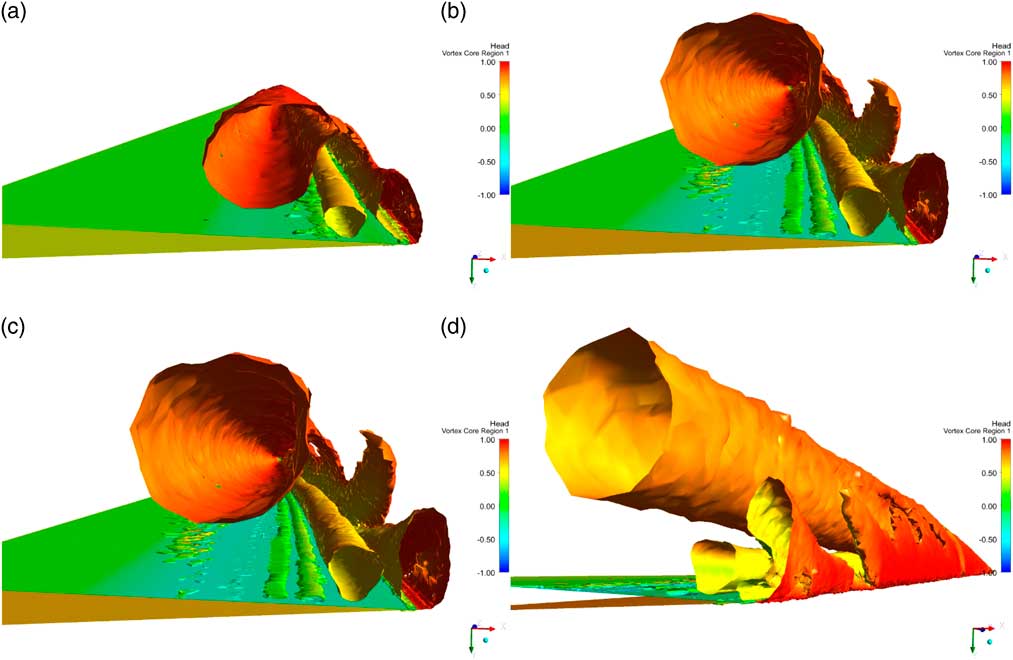
Figure 11 Vortex cores given by Q=0.002, (a) α=5º, (b) α=10º, (c) α=15º and (d) α=15º oblique view. Isosurface coloured by total head.

The inboard secondary vortex core, coloured in yellow in Fig. 11(a), is a secondary separation induced by an adverse pressure gradient created by the primary vortex, as described by Fink and Taylor⁽ Reference Fink and Taylor ^{18 )}, and directly modelled by Nutter⁽ Reference Nutter ^{9 )}. The outboard core, however, seems to be more akin to a viscous shear-induced recirculation caused by the interactions between the secondary separation and the primary vortex sheet. This structure is not visible in the measured data for the total head at α=5º in Fig. 2, although the recirculation is apparent at α=10º in Fig. 3 and α=15º in Fig. 4. The plots in Fig. 11 show this shear-induced recirculation becomes more elongated with a greater angle of incidence, with the development of a fingering structure in the primary vortex sheet. This is particularly apparent in the oblique view shown in Fig. 11(d) for α=15º. The movement outboard of the secondary separation with an increasing angle of incidence may compress the lower part of this recirculation, making it narrower and hence to have a greater tendency to develop an instability. The plots also indicate that because of the development of the fingering structures, the secondary shear-driven recirculation close to the leading edge can change considerably over a small downstream distance as these fingers develop.

Complementary information is provided by streamlines in Fig. 12. For each case, one set of streamlines is released from the leading edge of the wing, coloured by flow speed, and another set from a line inboard of the leading edge, in the shear-driven recirculation. The purpose of the second set is to highlight the secondary flow structure. To differentiate them from the first set, they are coloured in black. In this case, the view is not clipped at the measuring station, as interesting features develop in the streamlines downstream. The key feature that emerges from these plots is the clustering of the streamlines arising from the fingering structures shown in Fig. 11. This initiation of the clustering moves upstream and becomes more apparent as the angle of incidence increases. The implications of this are discussed later.

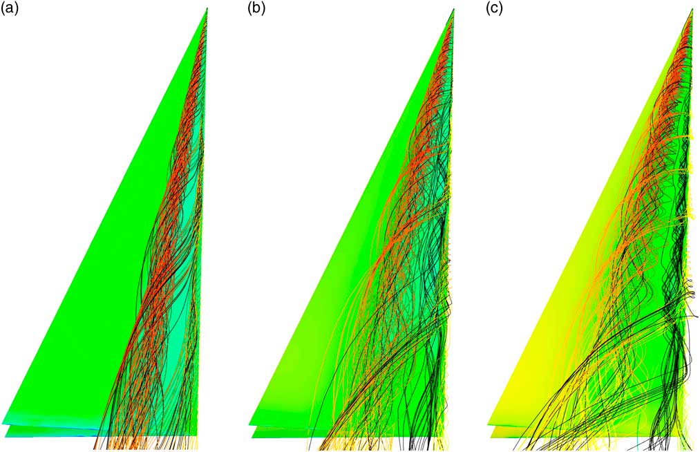
Figure 12 Streamlines, (a) α=5º, (b) α=10º and (c) α=15º

7.2 Marsden, Simpson and Rainbird configuration

Figure 13(a) and (b) shows the vortex cores for this configuration for α=8.8º and α=14º. The plots are clipped at Station 2, where the contour plots of the total head are available, and the same view is used for both plots.

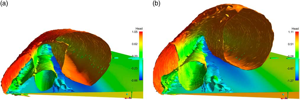
Figure 13 Vortex cores, Q= 0.002, coloured by total head, with the view clipped at Station 2: (a) α=8.8º and (b) α=14º. The wing surface is coloured by pressure.

Overall, the flow structures are similar to those shown by Fink and Taylor, with a primary leading-edge vortex sheet and core, the secondary separation induced by the primary vortex and a viscous shear-driven recirculation between the primary vortex sheet and the secondary separation. Additional weaker cores can be seen in the thickening boundary layer below and slightly outboard of the primary vortex and inboard of the secondary separation. These effects are also visible in the contours of the total head shown in Figs 9(a) and 10(a) at Station 2. The vortex cores also show the shear-driven recirculation elongates with an increasing angle of incidence.

The streamlines for these cases show similar structures and are given in the Supplementary information⁽ Reference Jones and Riley ^{13 )}.

8.0 QUALITATIVE COMPARISONS WITH OTHER DATA

Several other authors have presented vortex sheet data for slender delta wings. Liu et al. ⁽ Reference Liu, Makhmalbaf, Vewen Ramasamy, Kode and Merati ^{24 )} and Woodinga and Liu.⁽ Reference Woodinga and Liu ^{25 )} have investigated the flow over a 65° delta wing at a Reynolds number based on root chord of 4.1E4 in a water tunnel and in air at 4.4E5. The objective of their investigations was to demonstrate techniques for the extraction of skin friction fields, from surface luminescent dye visualizations in water and Global Luminescent Oil Film (GLOF) in air. These skin friction fields can be used to help identify the topological structure of the flow fields. The results in water presented by Liu et al. were consistent with surface GLOF measurements and with particle image velocimetry (PIV) of the flow field. A CFD model for the Liu⁽ Reference Liu, Makhmalbaf, Vewen Ramasamy, Kode and Merati ^{24 )} case was set up, using the methodology summarised earlier. The results are very similar to those described earlier in this paper. Apart from the skin friction fields, Liu et al.⁽ Reference Liu, Makhmalbaf, Vewen Ramasamy, Kode and Merati ^{24 )} only presented limited information on the flow field. In their PIV results, the secondary vortices were randomly ‘jittered’ by an appreciable amount. It was not possible therefore to use these PIV results for a quantitative comparison of the secondary flow structure, although they can be used for comparisons of primary vortex core locations. Details of the setup and a comparison with the data for the skin friction fields and separation lines, as well as with snapshots of the flow velocities from the PIV are given in the Supplementary Information⁽ Reference Jones and Riley ^{13 )}. These indicate that the CFD is reproducing the key features and qualitatively consistent with the data.

Smith⁽ Reference Smith ^{5 )} compares results for the measured primary vortex core location with those of Fink and Taylor⁽ Reference Fink and Taylor ^{18 )}, Marsden, Simpson and Rainbird⁽ Reference Marsden, Simpson and Rainbird ^{19 )} and with other data. Lowson⁽ Reference Lowson ^{20 )} extends the comparison to include results from his own smoke visualisations with no fewer than 10 separate measurements. Using this comparison, Kirkkopru and Riley⁽ Reference Kirkkopru and Riley ^{10 )} obtained bounds for the measured data, which they compared with results from their hybrid vortex sheet model. Figure 14 compares the primary vortex core location against the normalised angle of incidence from the data of Fink and Taylor, Marsden, Simpson and Rainbird, and Liu et al. with the corresponding CFD results; CFD (FT), CFD (MSR) and CFD (Liu), respectively, and the data bounds presented by Kirkkopru and Riley (Data Upper and Data Lower). The figures also include the predictions from the vortex sheet model of Smith, the hybrid vortex sheet model of Kirkkopru and Riley⁽ Reference Kirkkopru and Riley ^{10 )} (K&R) and the free-slip model from the CFD.

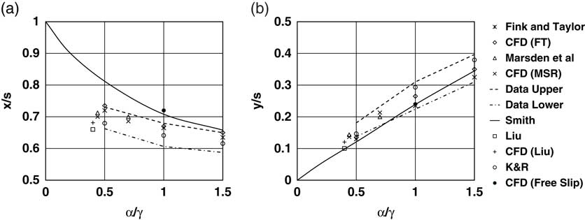
Figure 14 Comparisons of primary vortex core location with measured data, CFD and vortex sheet models, (a) lateral location and (b) vertical location.

The current CFD results are close to the corresponding measured values, and within the data bounds of the cases discussed by Lowson. The free-slip CFD model is in agreement with the vortex sheet model results of Smith⁽ Reference Smith ^{5 )} with the predicted vortex core further outboard than the data in Fig. 14(a), but within the data bounds vertically in Fig. 14(b). The results from the hybrid boundary-layer vortex sheet model of Kirkkopru and Riley are consistent with the measured data and the CFD.