


1. Introduction
Aerodynamic heating is a key issue in hypersonic flow research due to its strong relevance to the safety of ultrahigh-speed flight. The corresponding thermal protection design remains one of the major technical challenges before such flights will become practical. Under real flight conditions, laminar-to-turbulent transition is one of the most important sources of uncertain aerodynamic heating that might adversely impact a vehicle (Fedorov Reference Fedorov2011; Lee & Chen Reference Lee and Chen2019; Lee & Jiang Reference Lee and Jiang2019). Accurate knowledge of the interchange between mechanical and thermal energy within the production of wall-bounded turbulence is crucially important to the design of thermal protection systems. This paper reports an aerodynamic cooling phenomenon over a smooth-surface model based on the previously discovered dilatational-wave-induced heating mechanism (Zhu et al. Reference Zhu, Chen, Wu, Chen, Lee and Gad-el-Hak2018a,Reference Zhu, Lee, Chen, Wu, Chen and Gad-el-Hakb).
1.1. Thermal effect of the second-mode instability
An important mechanism in the transition process, absent in low-Mach-number flows, is the instability of second and higher modes, which was first identified based on linear stability analysis of hypersonic boundary layers (Mack Reference Mack1969). These modes play an increasingly important role as the Mach number increases, as demonstrated in previous studies (Stetson et al. Reference Stetson, Thompson, Donaldson and Siler1983, Reference Stetson, Thompson, Donaldson and Siler1984, Reference Stetson, Thompson, Donaldson and Siler1985; Stetson & Kimmel Reference Stetson and Kimmel1992; Bountin, Shiplyuk & Sidorenko Reference Bountin, Shiplyuk and Sidorenko2000; Fujii Reference Fujii2006; Zhang, Tang & Lee Reference Zhang, Tang and Lee2013; Casper, Beresh & Schneider Reference Casper, Beresh and Schneider2014; Sivasubramanian & Fasel Reference Sivasubramanian and Fasel2014, Reference Sivasubramanian and Fasel2015; Zhang et al. Reference Zhang, Zhu, Chen, Yuan, Wu, Chen, Lee and Gad-el-hak2015; Zhu et al. Reference Zhu, Zhang, Chen, Yuan, Wu, Chen, Lee and Gad-el-Hak2016). Along the streamwise direction, this instability mode initially grows according to linear stability theory (LST) (Malik & Spall Reference Malik and Spall1991; Stetson & Kimmel Reference Stetson and Kimmel1992), then saturates due to nonlinear interactions and finally decays before the flow becomes completely turbulent. This evolution process can be investigated via experiments (Shiplyuk et al. Reference Shiplyuk, Bountin, Maslov and Chokani2003; Zhu et al. Reference Zhu, Zhang, Chen, Yuan, Wu, Chen, Lee and Gad-el-Hak2016; Craig et al. Reference Craig, Humble, Hofferth and Saric2019) and direct numerical simulation (DNS) of the Navier–Stokes equations (Pruett & Chang Reference Pruett and Chang1998; Li, Fu & Ma Reference Li, Fu and Ma2010; Zhong & Wang Reference Zhong and Wang2012; Sivasubramanian & Fasel Reference Sivasubramanian and Fasel2014, Reference Sivasubramanian and Fasel2015; Zhu et al. Reference Zhu, Lee, Chen, Wu, Chen and Gad-el-Hak2018b). The thermal effect of the second-mode instability is also of concern. Schneider and co-workers (Berridge et al. Reference Berridge, Chou, Ward, Steen, Gilbert, Juliano, Schneider and Gronvall2010) were the first to observe hot streaks during the early stage of transition over a Mach 6 flared cone under quiet flow conditions, corresponding to an additional peak value (denoted as HR) in the spanwise-averaged temperature.  $\textrm {PCB}^{\circledR }$ piezoelectric pressure sensors have also indicated the appearance of a second-mode instability in that region. Sivasubramanian & Fasel (Reference Sivasubramanian and Fasel2015) used DNS to simulate the experiment of Berridge et al. (Reference Berridge, Chou, Ward, Steen, Gilbert, Juliano, Schneider and Gronvall2010). Streamwise hot streaks were also observed before the boundary layer became turbulent. Both spanwise-averaged heat transfer and that along a single streak exhibited hot region HR along the streamwise direction. Franko & Lele (Reference Franko and Lele2013) investigated the transition mechanisms of a Mach 6 planar hypersonic boundary layer. Three such mechanisms were identified, namely first-mode oblique interaction, second-mode fundamental resonance and second-mode oblique interaction. In the second and third cases, an additional peak heat transfer, hot region HR, appeared where the second mode reached its maximum. Note that the Stanton number at the hot region HR was slightly higher than that in the turbulent region, but the skin friction of the former was only half that of the latter, so a new aerodynamic heating mechanism might be active.
With the use of near-wall particle image velocimetry, Zhu et al. (Reference Zhu, Zhang, Chen, Yuan, Wu, Chen, Lee and Gad-el-Hak2016) obtained the transitional flow field over a Mach 6 flared cone, and found that the second-mode instability was correlated with the strong dilatation process. Zhu et al. (Reference Zhu, Chen, Wu, Chen, Lee and Gad-el-Hak2018a) then conducted experiments using the same model sprayed with temperature-sensitive paint and flush-mounted with  $\textrm {PCB}^{\circledR }$ piezoelectric pressure sensors along one centreline. The surface temperature distribution and instability amplitude evolution were simultaneously measured at different Reynolds numbers. They found that, as the Reynolds number increased, the hot region HR became stronger and stronger, appearing at the position where the second-mode amplitude reached its maximum value. Zhu et al. (Reference Zhu, Lee, Chen, Wu, Chen and Gad-el-Hak2018b) then conducted both particle image velocimetry and DNS investigations using this model. The aerodynamic heating ratios were calculated from the following equation:
 \begin{equation} W=-p\theta + \mu D:D + \left(\mu_b+\frac{4\mu}{3}\right)\theta^2, \end{equation}
where  $W$,
$W$,  $p$,
$p$,  $\theta$,
  $D$,
$D$,  $\mu$ and
  $\mu _b$ denote the aerodynamic heating ratio, pressure, dilatation, symmetric part of the velocity gradient tensor, first viscous coefficient and bulk viscous coefficient, respectively. Here,
 \begin{gather} \theta=\frac{\partial u_i}{x_i}, \end{gather}
 \begin{gather}D=\frac{1}{2}\left(\frac{\partial u_i}{x_j}+\frac{\partial u_j}{x_i}\right), \end{gather}
where ( $x_1, x_2, x_3$) and (
 $u_1, u_2, u_3$) represent the coordinate and velocity vectors, respectively. The three terms on the right-hand side of (1.1) are, in turn, the pressure dilatation, shear-induced viscous dissipation and dilatation-induced dissipation. The results showed that the time-averaged pressure dilatation
  $\langle w_{p\theta }\rangle =\langle -p\theta \rangle$ dominates the second-mode-induced aerodynamic heating. Because the newly discovered mechanism was different from the traditional theory that aerodynamic heating mainly arose from viscous dissipation, it was described as a ‘new principle for aerodynamic heating’ (Sun & Oran Reference Sun and Oran2018). Recently, Si et al. (Reference Si, Huang, Zhu, Chen and Lee2019) conducted experiments which showed that a wavy wall can suppress the second-mode instability, and consequently eliminate the hot region HR, further validating the new finding. Kuehl (Reference Kuehl2018) has recently proposed a thermoacoustic interpretation of the second-mode instability. By applying a one-dimensional parallel flow cycle-averaged disturbance acoustic energy equation, he showed that the second-mode growth was consistent with the standing-wave thermoacoustically driven instability. Mittal & Girimaji (Reference Mittal and Girimaji2020) used DNS to study the influence of pressure dilatation on internal energy evolution, kinetic internal energy exchange and kinetic energy spectrum evolution. The pressure dilatation leads to energy equipartitioning between the dilatational kinetic energy and internal energy.
In (1.1),  $\langle w_{p\theta }\rangle$ is reversible. For a periodically fluctuating flow, the sign of
  $\langle w_{p\theta }\rangle$ depends on the phase difference between the pressure and dilatation waves
  $\phi _{p\theta }$, that is,
 \begin{equation} \langle w_{p\theta}\rangle \left\{\begin{array}{@{}ll} >0, & \phi_{p\theta}<90^{\circ},\\ =0, & \phi_{p\theta}=90^{\circ},\\ <0, & \phi_{p\theta}>90^{\circ}. \end{array}\right. \end{equation}
One question that naturally arises is whether  $w_{p\theta }$ can switch to an opposite cooling process in hypersonic boundary layers, because it is reversible in (1.1); if so, a second question is how to artificially switch the direction of
  $w_{p\theta }$. Previous DNS results (Franko & Lele Reference Franko and Lele2013) have indicated a cooled region (denoted as CR) downstream of the hot region HR. The heat transfer to the body at the cooled region HR was observed to be lower than that in the laminar state, but the skin friction of the former was higher than that of the latter; this phenomenon has not been experimentally observed (see figure S1 in the supplementary material available at https://doi.org/10.1017/jfm.2020.1044). One possible reason is that the temperature-sensitive paint previously used by Zhu et al. (Reference Zhu, Chen, Wu, Chen, Lee and Gad-el-Hak2018a,Reference Zhu, Lee, Chen, Wu, Chen and Gad-el-Hakb) had a low temperature resolution (about 0.5 K). High-resolution temperature measurement techniques might help to investigate the cooling phenomenon.
1.2. Hypersonic flows over a porous surface
Malmuth et al. (Reference Malmuth, Fedorovf, Shalaevt, Cole, Khokhlov, Hites and Williams1998) exploited the behaviour of the hypersonic boundary layer as an acoustic waveguide, whereby the acoustic rays are reflected by the wall and turn around near the sonic line. They used stability theory for inviscid disturbances to examine whether the absorption of acoustic energy by an ultrasonically absorptive coating could stabilize the second and higher modes. Rasheed et al. (Reference Rasheed, Hornung, Fedorov and Malmuth2001) then performed a wind tunnel test in which the transition in the hypersonic boundary layer was successfully delayed using a porous surface. Fedorov et al. (Reference Fedorov, Malmuth, Rasheed and Hornung2001) further considered the viscous effect and studied the stabilization mechanism of an absorptive skin microstructure in the hypersonic boundary layer. They derived the acoustic admittance of the porous layer as the analytical form of the boundary conditions at the wall, and solved the eigenvalue problem based on viscous LST. Their analysis showed a reduction in the second-mode amplification due to the absorption of disturbance energy by the porous layer, which agreed with the experimental observations of Rasheed et al. (Reference Rasheed, Hornung, Fedorov and Malmuth2001). Fedorov et al. (Reference Fedorov, Shiplyuk, Maslov, Burov and Malmuth2003) then studied a fibrous absorbent material as the porous surface, and found that this strongly stabilized the second mode but destabilized the first mode. Chokani et al. (Reference Chokani, Bountin, Shiplyuk and Maslov2005) conducted an experimental study of the effects of a porous coating on the nonlinearity of the second mode using bispectral analysis, and found that the harmonics were greatly reduced by the porous layer. In contrast, an amplification of the second mode by the porous surface was also observed. Although the porous surface was designed to dampen the second mode based on numerical simulations, neither a significant damping of the second mode nor a delay of the transition process occurred. On the contrary, the results indicate an amplification of the second mode and an earlier transition. Recently, Zhu et al. (Reference Zhu, Shi, Zhu and Lee2019a) performed experiments comparing the stability of the boundary layer over a permeable-steel flared cone with that over one with a smooth surface. They found that the former produced a larger second mode than the latter. Furthermore, bispectral analysis showed weaker second-mode nonlinear interactions in the former case than in the latter. The porous material provides a sound admittance  $\tilde {k}$ as a boundary condition, that is,
 \begin{equation} p^\prime=\frac{1}{\tilde{k}}v^\prime,\quad \textrm{at}\ y = 0, \end{equation}
where  $p^\prime$ and
  $v^\prime$ denote the fluctuations of the pressure and normal velocity, respectively. Wang & Zhong (Reference Wang and Zhong2011) studied the effect of the phase angle of
  $\tilde {k}$ on the stability. They found that the phase difference of the first and second modes could be modified using the phase angle of
  $\tilde {k}$. This indicates that a porous surface can modify the phase difference between the pressure and the velocity near the wall.
This paper reports the results of a combined experimental, numerical and theoretical study of the evolution of the instability mode over both a smooth-surface and a porous-surface flared cone immersed in a Mach 6 flow and their relevance to surface temperature. The present study not only confirms the previously observed cooling phenomenon in the second-mode-dominated transition process, in which the phase angle  $\phi _{p\theta }$ plays an key role in the interchange between mechanical and thermal energy, but also presents the possibility of controlling
  $\phi _{p\theta }$ by modifying the surface sound admittance.
2. Experimental set-up
2.1. Facility
The experiments were carried out in a Mach 6 wind tunnel (M6QT) at Peking University, which is presently one of only three operational hypersonic quiet wind tunnels in the world (Schneider Reference Schneider2013). The tunnel has an open-jet configuration with a nozzle exit diameter of  $120$ mm. Owing to the small free-stream disturbances and upper limit of the unit Reynolds number under quiet conditions, no natural transition occurs up to the end of the model. Therefore, to obtain a complete picture of the transition process, the present study ran the wind tunnel under noisy conditions with the suction valve closed. Disturbances in hypersonic wind tunnels are dominated by sound waves, which are radiated by the turbulent boundary layers of the nozzle walls (Kovasznay Reference Kovasznay1953; Laufer Reference Laufer1961). A measurement of the normalized Pitot pressure is the standard method of characterizing the free-stream disturbance level in the test section (Stainback Reference Stainback1972). As introduced by Beckwith & Moore (Reference Beckwith and Moore1982), the free-stream disturbance level in our experiments was evaluated using a Kulite XCQ-062-25 pressure transducer that was flush-mounted in the tapered tip of a stainless steel rod and located at the centre of the nozzle exit. The transducer has a diameter of
  $2.57$ mm and a nominal resonant frequency of
  $150$ kHz. The initial output signal was amplified by a factor of 100 using a Donghua model DH3842 unit with a bandwidth of
  $300$ kHz, and sampled with a Donghua model DH5939 data acquisition system. During a typical test time of
  $20$ s, the stagnation pressure remained nearly constant, with a variation of less than
  $3\,\%$. The free-stream stagnation temperature and pressure were 430 K and 0.9 MPa, respectively. The free-stream velocity, unit Reynolds number, Mach number and pressure disturbance level were
  $870\ \textrm {m}\ \textrm {s}^{-1}$,
  $9.7\times 10^6$ m
 $^{-1}$, 6 and
  $2.2$ %, respectively.
2.2. Model
The first model considered in the present study is a flared cone with a smooth surface, as shown in figure 1(a). The full length is  $L = 260\ \textrm {mm}$. Its geometry consists of a
  $5^\circ$ half-angle circular conical profile for the first 100 mm of axial distance, followed by a tangent flare of radius 931 mm until the base of the cone at the 260 mm axial position. The first 50 mm of length is made of stainless steel with a nominal radius of 50
  $\mathrm {\mu }\textrm {m}$. The 210-mm-long afterbody is made of polyetheretherketone (PEEK) plastic. The origin of the coordinate system is located at the cone tip, with
  $x$ being the streamwise coordinate along the cone surface,
  $y$ the coordinate normal to the cone surface,
  $z$ the transverse coordinate normal to the
  $x$–
$x$– $y$ plane and
  $l$ the axial coordinate.
  $\textrm {PCB}^{\circledR }$ 132A31 sensors are flush-mounted at
  $l=100$, 120, 140, 160, 170, 180, 190, 200, 210, 220 and 230 mm along one centreline of the model.

Figure 1. (a) Schematic of the smooth-surface model. (b,c) Schematic of the porous-steel model and its microscopic structure. The porous steel is produced by sintering metal powder with an average aggregate radius of approximately  $140\ \mathrm {\mu }\textrm {m}$ and an air volume ratio of 20 %–30 %. (d) Image showing the two points (red, blue) from which the instability amplitude and temperature are simultaneously measured at
  $x=135$ mm in the linear growth stage of the second mode. Next to the red point, a 30-mm-long thin film covering the upstream porous surface is shown, corresponding to the smooth surface.
The second model has the same profile as the smooth-surface model, with the first 100 mm of axial distance made of stainless steel and the rest made of porous PM-35-35 steel (figure 1b,c). This porous material is produced by sintering metal powder with an average aggregate radius of approximately  $140\ \mathrm {\mu }\textrm {m}$ and an air volume ratio of 20 %–30 %. To simultaneously compare the instability amplitude and surface temperature growth between the smooth and porous surfaces,
  $\textrm {PCB}^{\circledR }$ sensors are flush-mounted at two points on the porous surface at
  $l=135\ \textrm {mm}$ and then replaced by cylindrical plugs made of PEEK plastic to measure the surface temperature. The spanwise angle difference between the two points is
  $30^{\circ }$. A thin film with a thickness of 0.1 mm covers the upstream region of one point to reduce the permeability of the surface to that of a smooth surface (figure 1(d); the film is 30 mm long, 10 mm wide and 0.055 mm thick).
Each model is installed along the centreline of the nozzle with zero angle of attack. The tip is positioned 50 mm into the exit of the nozzle. The length of the flow field that is unaffected by the reflected Mach waves is more than 400 mm, which is sufficient to embed the whole length of the model.
2.3. Instability measurement
Surface-mounted  $\textrm {PCB}^{\circledR }$ fast-response sensors are a convenient tool for evaluating the evolution of instability waves in hypersonic wall-bounded flows (Fujii Reference Fujii2006; Zhang et al. Reference Zhang, Tang and Lee2013, Reference Zhang, Zhu, Chen, Yuan, Wu, Chen, Lee and Gad-el-hak2015; Zhu et al. Reference Zhu, Zhang, Chen, Yuan, Wu, Chen, Lee and Gad-el-Hak2016). In this study,
  $\textrm {PCB}^{\circledR }$ 132A31 sensors were flush-mounted along one ray of the model. These sensors are piezoelectric quartz sensors with a high-frequency response above 1 MHz and minimum resolution of 7 Pa. The sensors were high-pass-filtered so that only fluctuations above 11 kHz were measured. The sensor head has a diameter of 3.18 mm, but the effective sensing area is only about
  $0.581\ \textrm {mm}^2$. The signals from the
  $\textrm {PCB}^{\circledR }$ sensors were first processed by
  $\textrm {ICP}^{\circledR }$ signal conditioners and then recorded using a Donghua 5939 acquisition system with a sample rate of 1 MHz. The power spectrum density of each pressure time series was calculated using Welch's method and the amplitude spectrum was obtained as the square root of the power density spectrum.
2.4. Surface temperature measurement and flow visualization
The surface temperature of the PEEK plastic parts was measured using an ![]() T 620 infrared (IR) camera. This material has an IR emissivity of up to 0.99. The camera has a resolution of
T 620 infrared (IR) camera. This material has an IR emissivity of up to 0.99. The camera has a resolution of  $640 \times 480$ pixels, a sample rate of 10 Hz and a thermal sensitivity of 0.05 K or better. The surface heat flux can be calculated from the temperature time series using the one-dimensional approach of Cook & Felderman (Reference Cook and Felderman1965) with the equation
 \begin{equation} q_n=\sqrt{\frac{\rho C_p k}{\rm \pi}}\sum_{j=1}^n \frac{T_j+T_{j-1}}{\sqrt{t_n-t_j}-\sqrt{t_n-t_{j-1}}}, \end{equation}
where  $q_n$,
  $T_n$ and
  $t_n$ are the
  $n$ step of heat flux, surface temperature and time;
  $\rho$,
  $C_p$ and
  $k$ are the density, specific heat capacity and heat conductivity of the model surface material.
Rayleigh-scattering flow visualization offers clear information regarding the evolution of the structures in the boundary layer. This method was used by Smits & Lim (Reference Smits and Lim2000) to investigate various hypersonic flows. Carbon dioxide ( $\textrm {CO}_2$) gas was injected upstream of the test section. The mass injection rate of
  $\textrm {CO}_2$ was no more than 5 % of the free-stream flow. Owing to the very low static temperature of the hypersonic flow, the
  $\textrm {CO}_2$ gas changes phase to become minute, solid particles in the free stream. The particles scatter when illuminated by the laser, so that this region is white on the greyscale CCD image. The scattering is of Rayleigh type because the particle diameters are much smaller than the laser wavelength. The
  $\textrm {CO}_2$ particles sublimate to gas near the wall because of the relatively high temperature there. This region appears black on the CCD image. The line distinguishing the white and black regions is the condensation line. The particles were illuminated by a double-cavity Nd:YAG laser from Continuum, generating light pulses of 6 ns in duration at a wavelength of 532 nm, with a maximum energy of 2 J per pulse. The laser sheet was projected vertically from the top window of the test section and aligned with the top centreline of the cone. The thickness and width of the light sheet were 1 and 100 mm, respectively. The time delay of the laser pulses was set to
  $1\ \mathrm {\mu }\textrm {s}$ and the sample rate was 2.5 Hz. A
  $\textrm {PCO}^{\circledR }$ SensiCam QE CCD camera equipped with a
  $\textrm {Nikkor}^{\circledR }$ Micro 200 mm lens viewed the light scattered by the particles from a side window. The field of view was
  $34.26\ \textrm {mm}^2$.
The side window glasses for IR and flow visualization are made of germanium and quartz, respectively. Thus, the surface temperature measurement and flow visualization should be conducted separately. In this study, simultaneous instability and surface temperature measurements were carried out first, and then the flow visualization was conducted.
3. Numerical settings
3.1. Analysis based on LST
The stability characteristics along the direction normal to the wall are investigated, similar to the study of Chen, Zhu & Lee (Reference Chen, Zhu and Lee2017). The decomposition of the flow field is given by
 \begin{equation} q(x,y,z,t)=\bar{q}(y)+ q^\prime(y)=\bar{q}(y)+ \tilde{q}(y)\exp(\textrm{i}\alpha x+\textrm{i}\beta z-\textrm{i}\omega t)+\textrm{c.c.} \end{equation}
Here,  $q=(u_1, u_2, u_3, T, p)$ and
  $\bar {q}$ denote the basic states,
  $q^\prime$ denotes the disturbance,
  $\tilde {q}(y)$ is the shape function of the disturbance,
  $\alpha$ and
  $\beta$ represent the streamwise wavenumbers, respectively, and
  $\omega$ is the angular frequency. After inserting the above decompositions into the Navier–Stokes equations, subtracting the basic states and neglecting the non-parallel and nonlinear terms, the following eigenvalue problem is obtained:
 \begin{equation} L_1(x,\alpha, \beta, \omega)q(y) = 0. \end{equation}
Here,  $L_1$ is a linear operator that has been described in the literature (Chen et al. Reference Chen, Zhu and Lee2017). For the smooth-wall PEEK model, the boundary conditions are
 \begin{equation} \hat{u}=\hat{v}=\hat{w}=\frac{{\partial \hat{T}}}{\partial \eta}=0 \quad \textrm{at} \ \eta=0, \quad \hat{u}=\hat{v}=\hat{w}= \hat{T}=0 \quad \textrm{at}\ \eta \rightarrow \infty. \end{equation}
For the permeable wall covered/not covered with the thin film, the boundary conditions are, respectively,
 \begin{equation} \hat{u}=\hat{v}=\hat{w}=\hat{T}=0 \quad \textrm{at} \ \eta=0, \quad \hat{u}=\hat{v}=\hat{w}= \hat{T}=0 \quad \textrm{at}\ \eta \rightarrow \infty \end{equation}
and
 \begin{equation} \hat{u}=\hat{w}= \hat{T} =0, \quad \hat{v}=K\hat{p}\quad \textrm{at} \ \eta=0, \quad \hat{u}=\hat{v}=\hat{w}= \hat{T}=0 \quad \textrm{at}\ \eta \rightarrow \infty, \end{equation}
where  $K$ is the admittance of the permeable wall.
3.2. Direct numerical simulations
The DNS approach in this study consists of two steps: laminar (steady) flow simulation, including the bow shock and without any perturbation; and unsteady simulation of the transition flow. The steady-flow solution provides the initial and boundary conditions for the unsteady simulation. The Hoam-OpenCFD code, developed by Li et al. (Reference Li, Fu and Ma2010), is used for the simulations. In this code, the compressible Navier–Stokes equations are solved numerically using a high-order finite difference method. Convection terms are split using Steger–Warming splitting and are discretized with a seventh-order weighted essentially non-oscillatory scheme. An eighth-order central finite difference scheme is used for the viscous terms. A third-order total-variation-diminishing Runge–Kutta method is used for the time discretization. The computational domain for the unsteady (transition) simulations in the circumferential direction spanned from the  $0^\circ$ meridian plane to the
  $45^\circ$ plane. The mesh had a resolution (
 $\text {streamwise}\times \text {wall normal} \times \text {circumference}$) of
  $4000\times 200\times 500$ elements. For the inflow boundary and upper boundary, time-independent conditions were obtained from the steady simulation (first step). The upper boundary was perturbed by random velocity noise (in three directions) with a maximum amplitude of 1 %. Eighteen modes with amplitudes of 1 % were seeded at the inflow boundary. A non-reflecting boundary condition was used on the outflow boundary in the streamwise direction. A periodical boundary was used in the circumferential direction. For the wall boundary, an isothermal wall temperature was used together with the assumption that
  $\partial p/\partial y$ = 0 on the wall, and a second-order one-sided finite difference scheme was used to compute the wall pressure. The DNS was performed on the Tianhe-2 supercomputer at the Guangzhou Supercomputing Center.
4. Results and discussion
4.1. Smooth-surface model
4.1.1. Evolution of instability
The wind tunnel takes about 3 s from valve opening to reach the steady state (figure 2a) when the second-mode instability reaches its steady amplitude (figure 2b). Correspondingly, periodic flow structures continuously appear in the boundary layer (figure 2c3–c6), with a wavelength of twice the boundary layer thickness, which is a typical characteristic of the second mode.

Figure 2. (a) Variation of the stream's total pressure with time, with the wind tunnel starting at  $t =2.0\ \textrm {s}$. (b) Variation of the second mode's amplitude with time, normalized by its time-averaged value for
  $t>6\ \textrm {s}$, arising from a
  $\textrm {PCB}^{\circledR }$ sensor's pressure time series at
  $x=150\ \textrm {mm}$; the wind tunnel started at
  $t =2.0\ \textrm {s}$. (c1–c6) Flow visualization from
  $t = 3.6$ to
  $6\ \textrm {s}$ at 0.4 s time intervals; the wind tunnel started at
  $t = 2.0\ \textrm {s}$.
The instability is then experimentally measured by  $\textrm {PCB}^{\circledR }$ sensors at
  $l=100$, 120, 140, 160, 170, 180, 190, 200, 210, 220 and 230 mm. The experimental power spectrum distributions (PSDs) at
  $l=120$, 150, 170, 190 and 210 are compared with those from DNS in figure 3(a–e), and can be observed to be in good agreement. The values have been normalized according to those at
  $l = 100\ \textrm {mm}$. The frequency of the second mode, corresponding to the peak in each PSD, is about 350 kHz, which agrees with the value identified in previous studies (Zhu et al. Reference Zhu, Zhang, Chen, Yuan, Wu, Chen, Lee and Gad-el-Hak2016, Reference Zhu, Chen, Wu, Chen, Lee and Gad-el-Hak2018a,Reference Zhu, Lee, Chen, Wu, Chen and Gad-el-Hakb). The evolution of the experimental second-mode amplitude is plotted in figure 3(f). The amplitudes have been normalized according to the value at
  $l = 100\ \textrm {mm}$. As shown, the amplitudes follow the LST predictions up to
  $x = 140\ \textrm {mm}$ (denoted as linear growth stage), then nonlinear interactions lead to saturation at around
  $x = 170\ \textrm {mm}$, before a final decay stage (denoted as nonlinear growth) occurs; this agrees well with the DNS predictions.

Figure 3. Streamwise evolution of PSDs at (a) 120 mm, (b) 150 mm, (c) 170 mm, (d) 190 mm and (e) 210 mm based on  $\textrm {PCB}^{\circledR }$ sensor measurements and DNS. (f) Streamwise evolution of the second-mode amplitude measured by
  $\textrm {PCB}^{\circledR }$ sensors, which is compared to the LST and DNS results. The amplitudes are normalized by the value at
  $l = 100\ \textrm {mm}$.
4.1.2. Surface temperature and heating ratio
Figure 4 presents the rate of increase in the surface temperature from  $t = 3.6$ to
  $6\ \textrm {s}$, as measured by the IR camera (also see supplementary movie S1). There are three levels of the time scale discussed in this work. The first level is of
  $10^2\ \textrm {ms}$, related to the camera's sample period, reflecting the time variation of flow condition as the wind tunnel starts. The second level is of
  $10^1\ \textrm {ms}$, related to the camera's exposure time and the third level is of
  $10^{-3}\ \textrm {ms}$, related to the second-mode period. Note that the IR camera's exposure time is about 10
 $^4$ times the second-mode period; thus the so-called ‘instantaneous’ temperature and heat flux measured by the IR camera reflect a time-integrated value during every exposure time. We show in supplementary movie S2 that such an integration time is long enough to obtain an accurate time-averaged value. As shown, the appearance of the second mode leads to a heating impact peak on the surface, at approximately
  $l = 175\ \textrm {mm}$, as identified in previous studies (Zhu et al. Reference Zhu, Chen, Wu, Chen, Lee and Gad-el-Hak2018a,Reference Zhu, Lee, Chen, Wu, Chen and Gad-el-Hakb). As the second-mode amplitude increases, the heating impact becomes increasingly strong (figure 4b,c), before streamwise streak structures appear and become prominent downstream of the hot region HR (figure 4d–f). Such streaks were first observed by Schneider's group in a quiet wind tunnel (Berridge et al. Reference Berridge, Chou, Ward, Steen, Gilbert, Juliano, Schneider and Gronvall2010), and have been numerically reproduced by Fasel's group and our group (Sivasubramanian & Fasel Reference Sivasubramanian and Fasel2015; Zhu et al. Reference Zhu, Lee, Chen, Wu, Chen and Gad-el-Hak2018b); however, they were not observed in our previous experiments (Zhu et al. Reference Zhu, Chen, Wu, Chen, Lee and Gad-el-Hak2018a,Reference Zhu, Lee, Chen, Wu, Chen and Gad-el-Hakb). The most probable reason is that the IR camera used in the present study has a much higher temperature resolution than the temperature-sensitive paint used in previous work. The appearance of streaks indicates a strong three-dimensional nonlinear interaction (Sivasubramanian & Fasel Reference Sivasubramanian and Fasel2015; Zhu et al. Reference Zhu, Lee, Chen, Wu, Chen and Gad-el-Hak2018b). With the improvement in temperature resolution, a cooled region can be observed at approximately
  $x = 200\ \textrm {mm}$ (denoted as CR in figure 4f), a feature that was not observed in our previous experiments. Previous DNSs have indicated the existence of the cooled region CR downstream of the hot region HR, where the heat transfer to the body is lower than that in the laminar state (see figure S1, supplementary material) (Franko & Lele Reference Franko and Lele2013). Note that the cooled region appears at approximately
  $x = 200\ \textrm {mm}$ (figure 4f), where the second-mode instability has decayed to approximately one-third of its maximum value (figure 3f), and is thus part of the nonlinear stage. The physical mechanism that causes this cooled region CR is the focus of the present work.

Figure 4. Rates of increase in surface temperature measured by the IR camera from  $t = 3.6$ to
  $6\ \textrm {s}$ at 0.4 s time intervals; the wind tunnel started at
  $t = 2.0\ \textrm {s}$. Both streak structures and negative rates of growth in temperature (denoted as CR) are observed in (f).
The DNS provides a good prediction of the second-mode instability relative to the experimental results (figure 3). A cooled region CR has been identified downstream of the hot region HR (see figure S1, supplementary material). As shown via DNS, although  $w_{p\theta }$ caused by the second-mode instability oscillates at a high frequency, its time-averaged value eventually approaches a steady value (see supplementary movie S2).
Figures 5(a) and 5(b) respectively present the distribution of cycle-averaged pressure dilatation  $\langle w_{p\theta }\rangle$ and viscous dissipation
  $\langle w_{vis}\rangle$ in the
  $x$–
$x$– $y$ plane. These quantities were calculated as
 \begin{gather} \langle w_{p\theta}\rangle =\frac{1}{NT}\int_0^{NT}-p\theta \,\textrm{d}t, \end{gather}
 \begin{gather}\langle w_{vis}\rangle =\frac{1}{NT}\int_0^{NT}\left(\mu D:D + \left(\mu_b+\frac{4\mu}{3}\right) \theta^2\right) \textrm{d}t, \end{gather}
where  $T$ and
  $N$ are the cycle time and cycle number of the second mode;
  $N =20$ and
  $\mu _b$=0 in our calculations. As shown,
  $\langle w_{vis}\rangle$ is positive beneath
  $y = 0.1\ \textrm {mm}$ for
  $x = 140\text {--}200\ \textrm {mm}$;
  $\langle w_{p\theta }\rangle$ is almost zero for
  $x < 140\ \textrm {mm}$. From
  $x = 140$ to
  $170\ \textrm {mm}$,
  $\langle w_{p\theta }\rangle$ becomes positive at approximately
  $y = 0.2\ \textrm {mm}$, corresponding to the heating impact HR. A negative region of
  $\langle w_{p\theta }\rangle$ occurs at approximately
  $y = 0.05\ \textrm {mm}$ for
  $x > 150\ \textrm {mm}$; in this region, the passing gas is able to cool. The cycle-averaged total heating ratio
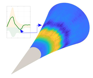
  $\langle w\rangle =\langle w_{p\theta }\rangle +\langle w_{vis}\rangle$ at
  $y = 0$ is given in figure 5(c); this agrees well with the streamwise evolution of the increase in surface temperature measured by the IR camera at
  $t = 6\ \textrm {s}$ (figure 5d). As indicated by the blue arrow, a region of negative
  $\langle w\rangle$ appears between
  $x = 180$ and 195 mm, where the cooling effect of
  $\langle w_{p\theta }\rangle$ is greater than the heating effect of
  $\langle w_{vis}\rangle$. This indicates that the cooled region CR in figures 4(f) and 5(d) is caused by the cooling effect of
  $\langle w_{p\theta }\rangle$.

Figure 5. Distributions of cycle-averaged (a) pressure dilatation  $w_{p\theta }$ and (b) viscous dissipation function
  $w_{vis}$. (c) Streamwise evolution of cycle-averaged
  $w_{p\theta }$,
  $w_{vis}$ and the total heating ratio
  $w=w_{p\theta }+w_{vis}$ at
  $y=0$, normalized according to the maximum value of
  $\langle w_{vis}\rangle$. (d) Streamwise evolution of increase in surface temperature arising from figure 4(f), normalized according to its maximum value. The cooled regions CR are indicated by blue arrows in (c,d).
The change in the sign of  $\langle w_{p\theta }\rangle$ is due to the variation in the phase difference
  $\phi _{p\theta }$, which can be evaluated by its cosine value:
 \begin{equation} \cos\phi_{p\theta}=\frac{\langle w_{p\theta}\rangle }{2p_{rms}\theta_{rms}}, \end{equation}
where  $p_{rms}$ and
  $\theta _{rms}$ are the root mean squares of the fluctuations in
  $p$ and
  $\theta$. We can calculate
  $\cos \phi _{p\theta }$ via both DNS and LST. For
  $x$ =130 mm, when the second-mode amplitude is relatively small and
  $p$ and
  $\theta$ behave sinusoidally, figure 6(a–c) shows that the DNS result agrees well with that of LST, indicating that
  $\cos \phi _{p\theta }$ is nearly zero, as shown in figure 6(c). This result is consistent with the thermoacoustic analysis of Kuehl (Reference Kuehl2018). As the second-mode amplitude increases sufficiently at
  $x = 150\ \textrm {mm}$, nonlinear interactions occur, deforming the curves of both
  $p$ and
  $\theta$ for
  $y > 0.05\ \textrm {mm}$ (figure 7b) and making
  $\cos \phi _{p\theta }$ much more positive compared to the LST prediction as shown in figure 7(d). As
  $x$ increases to 170 mm, harmonics with higher frequencies appear in the near-wall region (
 $y < 0.05\ \textrm {mm}$) and generate a negative value of
  $\cos \phi _{p\theta }$ (figure 8d; supplementary movie S2). This near-wall negative region extends for a long distance (
 $x = 190\ \textrm {mm}$) as the second-mode instability decays, as shown in figure 5(a). In general, the phase difference
  $\phi _{p\theta }$ determines the conversion direction of
  $\langle w_{p\theta }\rangle$. For the smooth-cone model, the second-mode instability in the linear stage contributes almost nothing to the thermal energy because
  $|\phi _{p\theta }| \approx 90^\circ$; nonlinear interactions can change
  $\cos \phi _{p\theta }$ in the second-mode instability, leading to aerodynamic heating or cooling.

Figure 6. Time series of the pressure fluctuation and dilatation at  $x = 130\ \textrm {mm}$ for (a)
  $y = 0.1\ \textrm {mm}$, (b)
  $y = 0.05\ \textrm {mm}$ and (c)
  $y = 0\ \textrm {mm}$, and (d) cosine value of phase difference
  $\phi _{p\theta }$. Here
  $T= 2.73\ \mathrm {\mu }\textrm {s}$ is the typical period of the second-mode instability.

Figure 7. Time series of the pressure fluctuation and dilatation at  $x = 150\ \textrm {mm}$ for (a)
  $y = 0.1\ \textrm {mm}$, (b)
  $y = 0.05\ \textrm {mm}$ and (c)
  $y = 0\ \textrm {mm}$, and (d) cosine value of phase difference
  $\phi _{p\theta }$. Here
  $T= 2.73\ \mathrm {\mu }\textrm {s}$ is the typical period of the second-mode instability.

Figure 8. Time series of the pressure fluctuation and dilatation at  $x = 170\ \textrm {mm}$ for (a)
  $y = 0.1\ \textrm {mm}$, (b)
  $y = 0.05\ \textrm {mm}$ and (c)
  $y = 0\ \textrm {mm}$, and (d) cosine value of phase difference
  $\phi _{p\theta }$. Here
  $T= 2.73\ \mathrm {\mu }\textrm {s}$ is the typical period of the second-mode instability.
4.2. Porous-surface model
It is now shown that  $\phi _{p\theta }$ can be artificially modified to control heat production. This initial work is currently limited to the linear growth stage of the second mode, where LST still applies. Porous materials have been widely used in the study of hypersonic boundary layers (Fedorov et al. Reference Fedorov, Malmuth, Rasheed and Hornung2001; Chokani et al. Reference Chokani, Bountin, Shiplyuk and Maslov2005; Maslov et al. Reference Maslov, Mironov, Poplavskaya and Kirilovskiy2005). Wang & Zhong (Reference Wang and Zhong2011) indicated that a porous surface can modify the phase difference between the pressure and the normal velocity near the wall; thus, a porous surface is considered below. Recently, sintered-steel models have been found to enhance the second-mode instability while suppressing its nonlinear interaction with harmonics (Zhu et al. Reference Zhu, Shi, Zhu and Lee2019b). Sintered steel is a porous material with an interconnected pore structure, allowing a gas to flow smoothly through the material. In the case of materials with irregular inner textures, multi-layered micro-perforated rigid-panel models with air gaps can describe the sound absorption properties of porous steel.
Similar to the deduction by Fedorov et al. (Reference Fedorov, Malmuth, Rasheed and Hornung2001), the value of  $k$ for materials with random pores can be expressed as
 \begin{equation} k=\frac{M_e \sqrt{T_w} \sqrt{{\rho}^{*}_w P^{*}_w}}{Z_n}, \end{equation}
where  $Z_n$ is the acoustic impedance of the permeable material. For the case of
  $n$ stacked layers, the impedance of the permeable material can be expressed as (Kim & Lee Reference Kim and Lee2010)
 \begin{equation} Z_n=z_a+\frac{Z_{n-1}Z(t_{air})}{Z_{n-1}+Z(t_{air})}, \end{equation}
where  $z_a$ is the impedance of a perforated panel and
  $t_{air}$ is the impedance of an air gap. Using classical models, the acoustic characteristics of porous materials with complicated pore shapes can be described (Stinson & Champoux Reference Stinson and Champoux1992; Allard & Daigle Reference Allard and Daigle2009). The multi-layered micro-perforated rigid-panel model considering air gaps can also provide good solutions, and is more convenient. Considering that the time dependence is
  $\exp (-\textrm {i} \omega t)$, consistent with the description of LST, the impedance of apertures can be expressed as
 \begin{equation} Z_a=-j\omega \rho_0 t_{panel} \left [1-\frac{2}{\beta \sqrt{j}}\frac{J_1(\beta \sqrt{j})}{J_0(\beta \sqrt{j})} \right]^{-1}. \end{equation}
This case does not consider the end effects associated with the aperture. For the real component of impedance,  $\sqrt {{\beta d}/{4 t_{panel}}}$ and
  ${8d}/{3 {\rm \pi}t_{panel}}$ should be added to the real and imaginary parts, respectively, of the thickness of the panels (Stinson & Shaw Reference Stinson and Shaw1985). For
  $1<\beta <10$, we have
 \begin{equation} Z_a \simeq \frac{32 \eta t_{panel}}{d^2} \sqrt{1+\frac{{\beta}^2}{32}}+ j \omega \rho_0 \left(1+\frac{1}{\sqrt{9+\dfrac{{\beta}^2}{2}}} \right). \end{equation}
The impedance of the apertures then becomes
 \begin{equation} Z_a=-j\omega \rho_0 t_{panel} \left [1-\frac{2}{\beta \sqrt{j}}\frac{J_1(\beta \sqrt{j})}{J_0(\beta \sqrt{j})} \right]^{-1} + \frac{32 \eta }{d^2} \sqrt{\frac{\beta d}{4 t_{panel}}}+ j \omega \rho_0 \frac{8d}{3 {\rm \pi}t_{panel}}. \end{equation}
Considering the effects of the gradation of aggregates and the target void ratio in acoustic absorption modelling, the impedance of a perforated panel becomes
 \begin{equation} z_a=\frac{Z_a}{P_{eff}}, \end{equation}
where  $P_{eff}=mP_{origin}$ can be considered as a reference for determining the effective perforated ratio. From the simplified aggregates model,
  $P_{origin} =({\sqrt {3}-{{\rm \pi} }/{2}})/\sqrt {3}$. However, to reflect the real pore distribution on the surface of porous media, it is necessary to adjust this parameter by a factor of
  $m$.
$m$.
Based on the model of a stacked assemblage of sphere-shaped aggregates, the thickness of the panel is  $t_{panel}=2({2\sqrt {6}}/{3}-1 )r\simeq 1.266r$, and the thickness of the air gaps
  $t_{air}$ can be expressed as
  $t_{air}=\kappa (r-{t}/{2})$.
This kind of permeable material, PM-35-35, is produced by rolling and sintering metal powders of various grain sizes. The radius of the aggregates  $r$ is assumed to be the average gradation, and has a value of about
  $140\ \mathrm {\mu }\textrm {m}$, the diameter of the apertures is chosen as
  $35\ \mathrm {\mu }\textrm {m}$ and the porous steel is 20 %–30 % air by volume. In the calculations,
  $m$ and
  $\kappa$ are set to 1.
As shown in figure 1(d),  $\textrm {PCB}^{\circledR }$ sensors were flush-mounted at two points
  $x = 135\ \textrm {mm}$ downstream on the porous and smooth surfaces to measure the instability. The sensors were then replaced by PEEK plugs to measure the surface temperatures using the IR camera. The value of
  $k$ was validated by substituting it into the LST calculations and comparing the instability with that observed during the experiments. Figure 9(a) compares the instability spectra at
  $x = 135\ \textrm {mm}$ (where LST still applies) given by the
  $\textrm {PCB}^{\circledR }$ sensor measurements with those produced by the LST calculations. It is clear that the two sets of results are in good agreement. As shown, the second-mode instability has frequencies of approximately 315 and 345 kHz over the porous and smooth surfaces, respectively. The second-mode instability amplitude is 66 % larger over the porous surface than over the smooth surface. Based on the LST calculations, the porous surface modifies
  $\cos \phi _{p\theta }$ to be negative at
  $y < 0.1\ \textrm {mm}$, i.e. a control layer forms near the wall (figure 9b).

Figure 9. (a) Comparison of the normalized instability spectra over the smooth (red) and porous (blue) cones at  $x = 135\ \textrm {mm}$ based on both measurements (solid line) and LST calculations (dotted line). The spectral peak indicates the second-mode instability. (b) Comparison of
  $\cos \phi _{p\theta }$ at
  $x = 135\ \textrm {mm}$ between the smooth and porous cones based on LST calculations.
The thermal effect is demonstrated in figure 10(a), which shows the variation in heat flux at the two points as a function of the wind tunnel run time. When the wind tunnel starts, the downstream heat flux increases markedly in both the porous and smooth cases; the former grows faster than the latter. The wind tunnel reaches a steady state at approximately  $t = 4\ \textrm {s}$ when the second mode takes effect (figure 10a). At this point, the heat flux downstream of the smooth film keeps at about
  $4200\ \textrm {W}\ \textrm {m}^{-2}$; in contrast, the heat flux downstream of the porous surface decreases to about
  $3000\ \textrm {W}\ \textrm {m}^{-2}$, 28 % lower than that over the smooth film, indicating the existence of the cooling effect by
  $\langle w_{p\theta }\rangle$. From an energy conversion aspect,
  $\langle w_{p\theta }\rangle$ periodically converts thermal energy to mechanical energy, leading to a higher rate of growth in the second mode for the porous surface, as shown in figure 9(a). As
  $\cos \phi _{p\theta }$ becomes more negative, the amplitude of the second mode grows, further enhancing the cooling effect. These results indicate that, by precisely designing the sound admittance, the switch between the heating and cooling functions can be proportionally controlled according to different requirements.

Figure 10. Variation of (a) the heat flux over the permeable model and (b) the second-mode instability amplitude with time. The latter is normalized by its maximum value.
5. Conclusions
In this paper, we have presented the results of a study into the aerodynamic cooling phenomenon in hypersonic boundary layers over smooth- and porous-surface flared cones using a combination of experimental, numerical and theoretical methods. The evolution of instabilities and surface-temperature distributions was observed via physical and numerical experiments. The free-stream stagnation temperature and pressure were 430 K and 0.9 MPa, respectively. The free-stream velocity, unit Reynolds number and Mach number were  $870\ \textrm {m}\ \textrm {s}^{-1}$,
  $9.7\times 10^6$ m
 $^{-1}$ and 6, respectively. The results of this study not only confirm the appearance of a previously observed cooling region as the second mode decays over the smooth-surface model, but also suggest the possibility of artificially cooling the boundary layer using a porous surface. The experimental results show that a region with a negative increase in surface temperature (denoted as CR) appears downstream of the local peak (denoted as HR) as the second mode evolves over the smooth-surface model. The DNS results also produce this cooled region CR in which the surface temperature is lower than for the laminar solution. The heating ratio per unit volume of gas, including the pressure dilatation
  $w_{p\theta }=-p\theta$ and the viscous dissipation
  $w_{vis}=\mu D:D + (\mu _b+{4\mu }/{3}) \theta ^2$, was investigated over the smooth-surface model. The nonlinear interactions of the second mode lead to a change in the phase difference between the pressure and dilatation
  $\phi _{p\theta }$, resulting in
  $w_{p\theta }$ cooling at
  $y = 0$ and the formation of the cooled region CR because
  $w_{p\theta }+w_{vis}<0$. For the porous model, the sound admittance was evaluated using the multi-layered micro-perforated rigid-panel model and validated using LST. The results given by LST also show a negative value of
  $\cos \phi _{p\theta }$ near the porous wall. In the linear growth stage, the surface heat flux over the porous surface is 28 % lower than that over the smooth surface, demonstrating the cooling effect of the porous surface.
In general, this work has indicated that, by precisely designing the surface sound admittance, the switch between heating and cooling in high-water-based fluid systems can be proportionally controlled according to the requirements of a particular application. In future, we will extend our analysis to the nonlinear stage. In a broad sense, pressure dilatation occurs widely in compressible flows, both in nature and in engineering applications. These results provide insights into the thermal protection design of future hypersonic vehicles.
Supplementary material and movies
Supplementary material and movies are available at https://doi.org/10.1017/jfm.2020.1044.
Funding
This research is supported by the National Natural Science Foundation of China under grant nos. 109103010062, 10921202, 11632002, 11602005 and 91752202, and National Key Project GJXM92579.
Declaration of interests
The authors report no conflict of interest.


