1 Introduction
Some public sectors are switching pension systems from defined-benefit or defined-contribution plans to cash-balance plans. For example, Kansas Public Employees Retirement System provides cash-balance plans for new members who begin their membership on or after January 1, 2015. Employees who participate in the cash-balance plans in Kansas cannot select investments; instead, the investment strategies of the pension fund are directed by the Public Employees Retirement System. The cash-balance plans in Kansas guarantee an annual rate of return of 5.25%. If the realized return on pension investments is below the guaranteed return, the government must offset the shortfall. Many states, such as California, Illinois, Kentucky, Nebraska, and Texas, have also designed cash-balance plans with guaranteed interest credits to a segment of their state employees. The guaranteed interest credit rate could be a constant or it could link to a Treasury yield. On certain conditions, the participants of the cash-balance plans receive some excess dividends when the realized return on pension investments exceeds the guaranteed return. In this paper, we analyze the subjective value that the participant places on the guarantee embedded in cash-balance plans.
The liabilities of the guarantee are similar to those of put options in the financial market; therefore, prior studies have applied risk-neutral option pricing approaches to price the liabilities.Footnote 1 When using option pricing approaches, the related papers implicitly assume that (i) the pension contracts embedded with guarantees are tradable without any restriction at any time in the market, (ii) both the participant and the issuer of the pension contract can adopt trading strategies to dynamically replicate the liabilities of guarantees, and (iii) both the participant and the issuer agree on the guarantee value. In fact, some of these assumptions cannot be applied to the guarantee embedded in the pension plan because the guarantee is not traded in the financial market; rather, it is a contract to protect participants from poor investment performance. Employees who participate in the pension plan embedded with a guarantee cannot realize profits by trading guarantees, contrary to those who trade options or other financial derivatives in the market. For this reason, it is difficult for employees to obtain the reference price of the guarantee from the market. Every participant may subjectively value the guarantee, and the value of the guarantee subjectively placed by the participant would be inconsistent with the liabilities of the guarantee (or equivalently, the cost objectively derived by option pricing approaches).Footnote 2 This paper explores this inconsistency and provides policy implications.Footnote 3
To derive the subjective value, we refer to and modify the certainty-equivalence framework of Hall and Murphy (Reference Hall and Murphy2000). The participant contributes a proportion of his or her salary to the hypothetical individual account, and the contributions are invested in one pension portfolio. The participant is assumed to act as if (i) the investment in the pension fund would not be protected by guaranteed interest credits and (ii) he or she would receive an additional cash amount when participating in the pension plan. The subjective value is equal to the received cash amount, such that the expected utility under these two assumptions is identical to the maximum expected utility when the guarantee is attached to the pension plan and the participant does not receive an additional cash amount.
The numerical results of our study are noteworthy. Although objective costs derived by option pricing methods are unrelated to wealth allocation and risk aversion, the subjective value of the guarantee varies with these individual features. More importantly, with a set of reasonable parameter settings, the subjective value is lower than the objective cost in many scenarios. A subjective value that is too low, relative to the objective cost, indicates that the guarantee costs too much. For instance, suppose that the objective cost is $100 and the subjective value is $51. The subjective value of $51 means that the expected utility of a participant who is not protected by the guarantee, but who receives $51 in cash, would be equal to the maximum expected utility of the other participant who is protected by the guarantee but does not receive $51. In this example, because the potential liabilities of the guarantee are higher than the subjective value, we claim that the pension system potentially spends too much providing the guarantee.
Some special findings are also worth noting. It is likely that a non-negative subjective value is not available when the participant cannot share any excess dividends in the event that the realized return on the pension portfolio exceeds the guaranteed return. The inexistence of a non-negative subjective value implies that, even though the pension contract does not guarantee returns and the participant is not compensated by additional cash, the participant's expected utility is higher than it is in the case where the guarantee is embedded. Conversely, the subjective value could be higher than the objective cost when the participant is highly risk averse and shares all excess dividends, and when it is difficult to diversify the risk by trading. This finding reflects that the guarantee is valuable from some participants’ perspective under certain circumstances, and accordingly, it is worthwhile for the pension system to provide a guaranteed return to these participants.
This paper contributes to the existing literature in at least three ways. First, we introduce the framework from managerial compensation literature to the analysis of pension guarantees. The interdisciplinary application provides one feasible and rational avenue to analyze pension plans, especially when the pension plan is embedded with a guaranteed interest credit and the participant is not required to pay for the guarantee. Policy makers could follow this framework to analyze guarantees in cash-balance plans and evaluate pension reforms. Second, we demonstrate that the participant may not place values on the guarantee as high as the potential liabilities of the guarantee, a finding that provides important policy implications. When designing a guarantee in the pension plan, the public pension system usually estimates the liabilities of the guarantee for risk control or actuarial purposes. However, this estimation is not sufficient. By comparing the subjective value perceived by the participant and the objective cost, we could know whether the guarantee or the pension plan caters to the participant and whether the pension system potentially spends too much on the guarantee. Moreover, the pension system should concurrently consider how to distribute excess dividends to the participant to satisfy the participant and increase the subjective value of the guarantee as determined by the participant.
Third, we open new directions for research regarding cash-balance pension plans. Brown et al. (Reference Brown, Dybvig and Marshall2001) and Hardy et al. (Reference Hardy, Saunders and Zhu2014) derive the market value of the participant's cash-balance pension account. Clark and Schieber (Reference Clark and Schieber2004) analyze the impact on the employee's pension wealth when converting from a defined-benefit plan to a cash-balance or defined-contribution plan. Coronado and Copeland (Reference Coronado and Copeland2004); Niehaus and Yu (Reference Niehaus and Yu2005), and Harper and Treanor (Reference Harper and Treanor2014) analyze why firms convert from one pension plan to another, for example, from a defined-benefit plan to a cash-balance plan. Unlike prior papers, we theoretically analyze the guarantee in cash-balance plans from the participant's perspective. Further research could conduct a field survey to investigate the subjective value of the guarantee placed by the participants in cash-balance plans.
This paper is organized as follows. Section 2 describes the economic models used and the methods for deriving the subjective value. Section 3 reports our numerical results given a constant guaranteed interest credit rate. Section 4 analyzes the subjective value of the guarantee linked to a Treasury yield. Section 5 concludes the paper.
2 Methodology
2.1 Basic economic models
We assume that there are many assets or portfolios in the financial market. For the i-th asset, the per-share price is expressed as follows:
 $$S_{i,t + \Delta} = S_{i,t} \cdot \exp \left( {\left( {\mu _i - \displaystyle{1 \over 2}\sigma _i^2} \right)\Delta + \sigma _i B_{i,\Delta}} \right),$$
where Δ is the length of time interval; S
i,t
and
 $S_{i,t + \Delta}$
are the time-t and time-(t + Δ) prices, respectively;
$S_{i,t + \Delta}$
are the time-t and time-(t + Δ) prices, respectively;
 $\mu _i $
is the expected rate of return;
$\mu _i $
is the expected rate of return;
 $\sigma _i$
is return volatility; and
$\sigma _i$
is return volatility; and
 $B_{i,\Delta}$
is the standard Brownian motion followed by a normal distribution with a zero mean and a standard deviation of
$B_{i,\Delta}$
is the standard Brownian motion followed by a normal distribution with a zero mean and a standard deviation of
 $\sqrt \Delta $
. The correlation coefficient between
$\sqrt \Delta $
. The correlation coefficient between
 $B_{i,\Delta}$
and
$B_{i,\Delta}$
and
 $B_{j,\Delta}$
(i ≠ j) is ρ
ij
∈ [ −1, +1], which represents the correlation estimate between the returns on the i-th and j-th assets. The guarantee costs are objectively obtained from option pricing approaches with the assumption that the instantaneous rate of return on each asset is the risk-free rate (r). To derive the subjective value, we follow the assumption in Hall and Murphy (Reference Hall and Murphy2000) that
$B_{j,\Delta}$
(i ≠ j) is ρ
ij
∈ [ −1, +1], which represents the correlation estimate between the returns on the i-th and j-th assets. The guarantee costs are objectively obtained from option pricing approaches with the assumption that the instantaneous rate of return on each asset is the risk-free rate (r). To derive the subjective value, we follow the assumption in Hall and Murphy (Reference Hall and Murphy2000) that
 $\mu _i = r + \beta _i \cdot EP$
, where
$\mu _i = r + \beta _i \cdot EP$
, where
 $\beta _i$
is the systematic risk and EP is the equity premium. This setting means that the participant subjectively places values on the guarantee in the real world, where the expected rate of return is described by the capital asset pricing model.Footnote
4
$\beta _i$
is the systematic risk and EP is the equity premium. This setting means that the participant subjectively places values on the guarantee in the real world, where the expected rate of return is described by the capital asset pricing model.Footnote
4
At time 0, an employee works in a public sector and participates in a state-sponsored cash-balance pension plan. The employer contributes c
er
W
0 and the employee contributes c
ee
W
0 to a hypothetical individual account, where c
er
and c
ee
are the proportions between 0 and 1 and W
0 is the salary. The contributions are invested in a pension portfolio with a time 0 per-share price of
 $S_{p,0}$
. The pension portfolio is not selected by the employee but by the pension sponsor (e.g., the retirement system run by the state, the pension provider, or the third party managing the pension fund). The pension plan guarantees that the participant receives at least (c
er
+ c
ee
)W
0 · e
gT
at time T (the retirement date), where g is the constant guaranteed interest credit rate.Footnote
5
$S_{p,0}$
. The pension portfolio is not selected by the employee but by the pension sponsor (e.g., the retirement system run by the state, the pension provider, or the third party managing the pension fund). The pension plan guarantees that the participant receives at least (c
er
+ c
ee
)W
0 · e
gT
at time T (the retirement date), where g is the constant guaranteed interest credit rate.Footnote
5
Employee contributions are made on a pre-tax basis. After contributing c
ee
W
0 to the pension account, the participant has (1 − c
ee
)W
0, which is taxable at an income tax rate of τ. The participant spends δ proportion of the disposable income on expenditures, allocates α
G
proportion of the disposable income to the risk-free portfolio at a rate of return r, and invests another proportion of (1 − δ − α
G
) in the risky tradable portfolio with a time 0 per-share price of
 $S_{x,0}^G $
.Footnote
6
The expenditures at time 0 could be expressed as
$S_{x,0}^G $
.Footnote
6
The expenditures at time 0 could be expressed as
 $C_0= \delta (1 - \tau )\,(1 - c_{ee} )W_0 $
. The superscript of G in α
G
and
$C_0= \delta (1 - \tau )\,(1 - c_{ee} )W_0 $
. The superscript of G in α
G
and
 $S_x^G $
denotes that these variables are considered when the guarantee is embedded in the pension plan. The risky tradable portfolio is selected by the employee. The correlation coefficient between the rates of return on the pension portfolio and the risky tradable portfolio is described by
$S_x^G $
denotes that these variables are considered when the guarantee is embedded in the pension plan. The risky tradable portfolio is selected by the employee. The correlation coefficient between the rates of return on the pension portfolio and the risky tradable portfolio is described by
 $\rho _{px}^G $
. A more positive
$\rho _{px}^G $
. A more positive
 $\rho _{px}^G $
implies that the prices of the two portfolios move in a more similar direction and the participant's assets are less diversified. The participant is prohibited from trading the pension contract. At time T, the participant's total wealth is expressed as:
$\rho _{px}^G $
implies that the prices of the two portfolios move in a more similar direction and the participant's assets are less diversified. The participant is prohibited from trading the pension contract. At time T, the participant's total wealth is expressed as:
 $$\eqalign{W_T^G = \ & Max\left[ {(c_{er} + c_{ee} )W_0 \cdot e^{gT}, (c_{er} + c_{ee} )W_0 \cdot \left[ {e^{gT} + h \cdot \left( {\displaystyle{{S_{\,p,T}} \over {S_{\,p,0}}} - e^{gT}} \right)} \right]} \right] \cr & + (1 - \tau )(1 - c_{ee} )W_0 \cdot \left[ {\alpha ^G \cdot (1 + r)^T + (1 - \delta - \alpha ^G ) \cdot \displaystyle{{S_{x,T}^G} \over {S_{x,0}^G}}} \right],} $$
where
 $S_{p,T}$
and
$S_{p,T}$
and
 $S_{x,T}$
are the per-share price of the pension portfolio and the risky tradable portfolio, respectively, at time T. The term
$S_{x,T}$
are the per-share price of the pension portfolio and the risky tradable portfolio, respectively, at time T. The term
 $(c_{er} + c_{ee} )W_0 \cdot \left[ {e^{gT} + h \cdot \left( {(S_{p,T}/S_{p,0}) - e^{gT}} \right)} \right]$
is the amount that the participant receives at retirement if
$(c_{er} + c_{ee} )W_0 \cdot \left[ {e^{gT} + h \cdot \left( {(S_{p,T}/S_{p,0}) - e^{gT}} \right)} \right]$
is the amount that the participant receives at retirement if
 $S_{p,T}/S_{p,0}$
is higher than e
gT
. The difference between
$S_{p,T}/S_{p,0}$
is higher than e
gT
. The difference between
 $S_{p,T}/S_{p,0}$
and e
gT
is defined as the excess dividends from the pension portfolio. We assume that if the realized return on the pension portfolio exceeds the guaranteed return, the participant shares h proportion of the excess dividends. If h = 1,
$S_{p,T}/S_{p,0}$
and e
gT
is defined as the excess dividends from the pension portfolio. We assume that if the realized return on the pension portfolio exceeds the guaranteed return, the participant shares h proportion of the excess dividends. If h = 1,
 $(c_{er} + c_{ee} )W_0 \cdot \left[ {e^{gT} + h \cdot \left( {(S_{p,T}/S_{p,0}) - e^{gT}} \right)} \right]$
turns to
$(c_{er} + c_{ee} )W_0 \cdot \left[ {e^{gT} + h \cdot \left( {(S_{p,T}/S_{p,0}) - e^{gT}} \right)} \right]$
turns to
 $(c_{er} + c_{ee} )W_0 \cdot S_{p,T}/S_{p,0}$
, meaning that the participant shares all upside benefits of the pension portfolio when the realized return on the pension portfolio exceeds the guaranteed return. If
$(c_{er} + c_{ee} )W_0 \cdot S_{p,T}/S_{p,0}$
, meaning that the participant shares all upside benefits of the pension portfolio when the realized return on the pension portfolio exceeds the guaranteed return. If
 $S_{p,T}/S_{p,0}$
is lower than e
gT
, the pension system has to compensate for the shortfall equal to
$S_{p,T}/S_{p,0}$
is lower than e
gT
, the pension system has to compensate for the shortfall equal to
 $(c_{er} + c_{ee} )W_0 \cdot \left( {e^{gT} - (S_{p,T}/S_{p,0})} \right)$
. We could rewrite the shortfall for each dollar of contribution as
$(c_{er} + c_{ee} )W_0 \cdot \left( {e^{gT} - (S_{p,T}/S_{p,0})} \right)$
. We could rewrite the shortfall for each dollar of contribution as
 ${\rm Max}\left( {e^{gT} - (S_{p,T}/S_{p,0} ),0} \right)$
. Because the form of the shortfall is similar to the payoff of a put option traded in the financial market, the researchers and practitioners typically use option pricing models to estimate the potential liabilities of the guarantee.
${\rm Max}\left( {e^{gT} - (S_{p,T}/S_{p,0} ),0} \right)$
. Because the form of the shortfall is similar to the payoff of a put option traded in the financial market, the researchers and practitioners typically use option pricing models to estimate the potential liabilities of the guarantee.
2.2 Derivation of the subjective value
We refer to the concept in Hall and Murphy (Reference Hall and Murphy2000) to obtain the subjective value that the participant places on the guarantee at time 0. Hall and Murphy (Reference Hall and Murphy2000) analyze the value of non-tradable executive stock options (ESOs) subjectively placed by the risk-averse executive and show that the subjective value of an ESO is affected by many personal characteristics, such as asset allocation, risk aversion, etc. Firms grant ESOs to executives as remuneration without charging premiums. Because the payoffs of most ESOs are analogous to a vanilla call with a constant strike price, practitioners usually adopt the Black and Scholes (Reference Black and Scholes1973) formula to determine the costs of ESOs. Recently, many papers have indicated that it is inappropriate to value ESOs using the Black–Scholes formula because executives are not in the same situation as option holders who can freely trade options.Footnote 7 For example, executives cannot trade ESOs or hedge risks by selling the firm stock, i.e., the underlying asset of ESOs, at will. Moreover, executives are prohibited from trading and exercising options before the termination of the vesting period. This non-tradable feature of an ESO is also observed in the guarantee embedded in the pension plan. The guarantee embedded in the public cash-balance pension plan is offered by the government, and the employee or the participant does not pay premiums for it. Such a guarantee is not tradable, but rather, it is a contract that protects the participant. Therefore, we refer to Hall and Murphy (Reference Hall and Murphy2000) to evaluate the subjective value of the guarantee.
Suppose that the risk-averse participant's utility function is U(x) = x 1−A /(1 − A) for A ≠ 1 and U(x) = ln x for A = 1, where A is the relative risk aversion coefficient. If the participant received additional V in cash at time 0, instead of the guaranteed interest credit, and allocated that cash to expenditures and investments, then the participant's total wealth at the retirement date would be:
 $$\eqalign{& W_T^V = (1 - \eta )V \cdot Y + (c_{er} + c_{ee} )W_0 \cdot \displaystyle{{S_{\,p,T}} \over {S_{\,p,0}}} \cr & + (1 - \tau )(1 - c_{ee} )W_0 \cdot \left[ {\tilde \alpha \cdot (1 + r)^T + (1 - \delta - \tilde \alpha ) \cdot \displaystyle{{\tilde S_{x,T}} \over {\tilde S_{x,0}}}} \right].} $$
Equation (3) differs from equation (2) in three ways. First,
 $\tilde \alpha $
and
$\tilde \alpha $
and
 $\tilde S_x $
are considered in a scenario where the guarantee is not embedded in the pension plan. The difference in the notations indicates that the consumption and investment decisions when no guarantee is embedded are not necessarily the same as when the guarantee is embedded. Second,
$\tilde S_x $
are considered in a scenario where the guarantee is not embedded in the pension plan. The difference in the notations indicates that the consumption and investment decisions when no guarantee is embedded are not necessarily the same as when the guarantee is embedded. Second,
 $(c_{er} + c_{ee} )\,W_0 \cdot S_{p,T} /S_{p,0} $
denotes how much the participant would receive when bearing the downside risk and enjoying the upside benefits of the pension portfolio without the protection of the guaranteed interest credit. Third, after receiving the additional cash, the participant would allocate ηV to expenditures and (1-η)V to the risk-free asset or the risky portfolio. The setting of η allows us to analyze how the subjective value changes when the participant spends more on expenditures than
$(c_{er} + c_{ee} )\,W_0 \cdot S_{p,T} /S_{p,0} $
denotes how much the participant would receive when bearing the downside risk and enjoying the upside benefits of the pension portfolio without the protection of the guaranteed interest credit. Third, after receiving the additional cash, the participant would allocate ηV to expenditures and (1-η)V to the risk-free asset or the risky portfolio. The setting of η allows us to analyze how the subjective value changes when the participant spends more on expenditures than
 $C_0 $
. The expression (1 − η)V · Y reflects how much the participant would earn from investing all or a part of V in assets. If the participant invests in the risk-free asset, then Y = (1 + r)
T
. The risk-free asset herein is equipped with a non-negative rate of return and protects the participant from withdrawing nothing at retirement. We also consider the case where
$C_0 $
. The expression (1 − η)V · Y reflects how much the participant would earn from investing all or a part of V in assets. If the participant invests in the risk-free asset, then Y = (1 + r)
T
. The risk-free asset herein is equipped with a non-negative rate of return and protects the participant from withdrawing nothing at retirement. We also consider the case where
 $Y = \tilde S_{x,T} /\tilde S_{x,0} $
because it is likely that the participant would invest the extra V on the risky tradable portfolio.
$Y = \tilde S_{x,T} /\tilde S_{x,0} $
because it is likely that the participant would invest the extra V on the risky tradable portfolio.
As previously mentioned, the mix of (
 $\tilde \alpha, \tilde S_x $
) may differ from (
$\tilde \alpha, \tilde S_x $
) may differ from (
 $\alpha ^G, S_x^G $
). We consider this difference and obtain the subjective value by conducting the following steps:
$\alpha ^G, S_x^G $
). We consider this difference and obtain the subjective value by conducting the following steps:
Step A. Define the utility with the guaranteed interest credit as
 $$U^G = U(C_0 ) + e^{ - rT} U\left( {W_T^G} \right).$$
The utility level depends on the expenditures at time 0 and terminal wealth at time T. Derive the mix of
 ${\rm (}\alpha ^G, \beta _x^G, \sigma _x^G, \rho _{px}^G )$
to maximize the expected utility E
0 (U
G
), where E
0 (·) denotes the expectation function conditional on the market information up to time 0. The maximum of E
0 (U
G
) is denoted by
${\rm (}\alpha ^G, \beta _x^G, \sigma _x^G, \rho _{px}^G )$
to maximize the expected utility E
0 (U
G
), where E
0 (·) denotes the expectation function conditional on the market information up to time 0. The maximum of E
0 (U
G
) is denoted by
 $\overline {EU} ^G $
.
$\overline {EU} ^G $
.
Step B. Define the utility without the guaranteed interest credit but with the additional cash amount as
 $$UnoG = U(C_0 + \eta V) + e^{ - rT} U\left( {W_T^V} \right),$$
where the sum of
 $C_0 $
and ηV is the amount spent on expenditures at time 0. Derive the mix of
$C_0 $
and ηV is the amount spent on expenditures at time 0. Derive the mix of
 ${(\tilde \alpha, \tilde \beta _x, \tilde \sigma _x, \tilde \rho _{px} )}$
to maximize E
0 (UnoG|V = 0), which is the participant's expected utility when the pension system provides neither a guaranteed interest credit nor an additional cash amount. In this step, we assume that the participant determines the allocation between the risk-free asset and the risky portfolio before deriving the subjective value. In reality, the participant does not receive this additional cash amount, and hence it will be rational to determine the allocation under the assumption that V = 0.
${(\tilde \alpha, \tilde \beta _x, \tilde \sigma _x, \tilde \rho _{px} )}$
to maximize E
0 (UnoG|V = 0), which is the participant's expected utility when the pension system provides neither a guaranteed interest credit nor an additional cash amount. In this step, we assume that the participant determines the allocation between the risk-free asset and the risky portfolio before deriving the subjective value. In reality, the participant does not receive this additional cash amount, and hence it will be rational to determine the allocation under the assumption that V = 0.
Step C. The participant obtains V such that
 $$E_0 (\left. {UnoG} \right \vert \tilde \alpha, \tilde \beta _x, \tilde \sigma _x, \tilde \rho _{\,px} ) = \overline {EU} ^G, $$
conditioned on the mix of
 ${\rm (}\tilde \alpha, \tilde \beta _x, \tilde \sigma _x, \tilde \rho _{px} )$
derived in Step B with the constraint that V ≥ 0.
${\rm (}\tilde \alpha, \tilde \beta _x, \tilde \sigma _x, \tilde \rho _{px} )$
derived in Step B with the constraint that V ≥ 0.
As equation (6) considers the mix of
 ${\rm (}\tilde \alpha, \tilde \beta _x, \tilde \sigma _x, \tilde \rho _{px} )$
derived from Step B, the subjective value could be viewed as the maximum additional cash compensated by the employer such that the expected utility without the protection of the guarantee but with V in cash at time 0 is equal to the maximum expected utility with the guarantee. The non-negative constraint on V means that the participant should be compensated in exchange for the guarantee. If the subjective value is negative, the guarantee is meaningless because the expected utility without the guarantee and any additional compensation is even higher than the maximum expected utility with the guarantee.
${\rm (}\tilde \alpha, \tilde \beta _x, \tilde \sigma _x, \tilde \rho _{px} )$
derived from Step B, the subjective value could be viewed as the maximum additional cash compensated by the employer such that the expected utility without the protection of the guarantee but with V in cash at time 0 is equal to the maximum expected utility with the guarantee. The non-negative constraint on V means that the participant should be compensated in exchange for the guarantee. If the subjective value is negative, the guarantee is meaningless because the expected utility without the guarantee and any additional compensation is even higher than the maximum expected utility with the guarantee.
Deriving the closed-form formula for the subjective value is not an easy task. An alternative and more feasible way to obtain the subjective value is through simulation. The details of the simulation procedure are described in the Appendix.
3 Numerical results
To derive the numerical results, we simulate 100,000 paths with the parameterizations as summarized in Table 1. We set the annual guaranteed interest credit rate at 0.0525, the income tax rate at 0.15, and the time-0 salary at 1000. The contribution rate is 0.03 for the contribution made by the employer and 0.06 for the contribution made by the participant. The accumulation period is 20 years. The time-0 price of each portfolio is 1. According to equations (1) to (3), what is important is not the time-0 price of the portfolio but the rate of return, and therefore, the setting of the time-0 price of each portfolio does not affect our conclusions. The risk-free rate and the equity premium are cited from Graham and Harvey (Reference Graham and Harvey2013), where the December 2012 survey indicates that the 10-year bond yield is 0.0163 and the average risk premium is 0.0383. According to the data regarding consumer expenditures for July 2011 through June 2012 released by the U.S. Bureau of Labor Statistics (2013), the ratio of average annual expenditures to income before taxes is 0.777.Footnote 8 We assume δ = 0.8, which is higher than 0.777 because this paper defines δ as the proportion of the disposable income on expenditures. The relative risk aversion coefficients are not set at a high level since Branger et al. (Reference Branger, Mahayni and Schneider2010); Inkmann et al. (Reference Inkmann, Lopes and Michaelides2011); Wang and Young (Reference Wang and Young2011), and Gao and Ulm (Reference Gao and Ulm2012) use low relative risk aversion coefficients.
Table 1. Parameter estimates used in simulation
Note: The last seven symbols are used in the analysis of the relative guarantee in Section 4.
We consider three mixes of the beta and return volatility of the pension portfolio. Baker et al. (Reference Baker, Bradley and Wurgler2011) sort their samples into five quintiles and estimate betas and volatilities of each sub-sample. When sorting according to volatility, the second safe quintile is featured with a beta of 1.01 and a volatility of 0.1672. Therefore, we set
 $\beta _p = 1$
and
$\beta _p = 1$
and
 $\sigma _p = 0.16$
in one of our three mixes. Also according to Baker et al. (Reference Baker, Bradley and Wurgler2011), we set
$\sigma _p = 0.16$
in one of our three mixes. Also according to Baker et al. (Reference Baker, Bradley and Wurgler2011), we set
 $\beta _p = 0.75$
and
$\beta _p = 0.75$
and
 $\sigma _p = 0.131$
for the safest pension portfolio, and the mix of
$\sigma _p = 0.131$
for the safest pension portfolio, and the mix of
 $\beta _p = 1.71$
and
$\beta _p = 1.71$
and
 $\sigma _p = 0.32$
characterizes the riskiest pension portfolio.
$\sigma _p = 0.32$
characterizes the riskiest pension portfolio.
The allocations and the features of feasible risky assets that the participant would select to maximize the expected utility are as follows. We assume that α ∈{0, 0.05, 0.1, 0.15, 0.2}, and the participant would invest in the risky tradable portfolios with the following parameter settings: (i) β x = 0.75 and σ x ∈{0.14, 0.15, 0.16, …, 0.47, 0.48}; (ii) β x = 1 and σ x ∈{0.16, 0.17, 0.18, …, 0.49, 0.5}; and (iii) β x = 1.71 and σ x ∈{0.32, 0.33, 0.34, …, 0.59, 0.6}. We take two ranges of ρ px into consideration: ρ px ∈{−0.5, −0.4, …, 0.4, 0.5} and ρ px ∈{0.2, 0.3, 0.4, 0.5}. These settings generate 5,445 types of allocations if ρ px ∈{−0.5, −0.4, …, 0.4, 0.5} or 1,980 types of allocations if ρ px ∈{0.2, 0.3, 0.4, 0.5}. A more negative ρ px means that the prices of the pension portfolio and the risky tradable portfolio do not move similarly and that the risky tradable portfolio partially hedges the risks from the depreciation of the pension portfolio. We claim that the participant in the case of ρ px ∈{−0.5, −0.4, …, 0.4, 0.5} has more advantages in selecting investments to maximize the expected utility than in the case of ρ px ∈{0.2, 0.3, 0.4, 0.5}. These parameter settings cannot describe all allocations or portfolios in the market; nevertheless, these settings are reasonable, and the participant may not have proficient knowledge or enough time to pay attention to all portfolios.
Tables 2 and 3 report the objective costs and the ratios of the subjective value to the objective cost (namely as S/O ratios) under the assumptions that η = 0 and the participant would invest all additional cash in the risk-free asset or the risky tradable portfolio. The objective cost is derived by the equation:
 $$\eqalign{&(c_{er} + c_{ee} )W_0 \cdot E_0^Q \left[ {e^{ - rT} \cdot {\rm Max}\left( {e^{gT} - \displaystyle{{S_{\,p,T}} \over {S_{\,p,0}}}, 0} \right)} \right] \cr & \quad = (c_{er} + c_{ee} )W_0 \cdot \left( {e^{(g - r)T} N( - d_2 ) - N( - d_1 )} \right)},$$
where
 $E_0^Q ( \cdot )$
is the expectation function under the risk-neutral Q-measure conditional on the market information up to time 0,
$E_0^Q ( \cdot )$
is the expectation function under the risk-neutral Q-measure conditional on the market information up to time 0,
 $d_1 = (- gT + (r + 0.5\sigma _p^2 )T)/$
 $(\sigma _p \sqrt T ),d_2 = d_1 - \sigma _p \sqrt T $
, and N(·) is the cumulative distribution function of the standard normal distribution.
$(\sigma _p \sqrt T ),d_2 = d_1 - \sigma _p \sqrt T $
, and N(·) is the cumulative distribution function of the standard normal distribution.
Table 2. S/O ratios with η = 0, h = 100%, and a constant guarantee
Note: S/O is the ratio of the subjective value to the objective cost; η is the proportion of the additional cash amount on expenditures; h is the proportion of the excess dividends shared by the participant if the realized return on the pension portfolio exceeds the guaranteed return; A is the participant's relative risk aversion coefficient; ρ px is the correlation estimate between the returns on the pension portfolio and the risky tradable portfolio. At t = 0, all additional cash received in place of the guaranteed interest credit would be invested at the risk-free rate in case (i) or in the risky tradable portfolio in case (ii).
Table 3. S/O ratios with η = 0, h = 0, and a constant guarantee
Note: S/O is the ratio of the subjective value to the objective cost; η is the proportion of the additional cash amount on expenditures; h is the proportion of the excess dividends shared by the participant if the realized return on the pension portfolio exceeds the guaranteed return; A is the participant's relative risk aversion coefficient; ρ px is the correlation estimate between the returns on the pension portfolio and the risky tradable portfolio. At t = 0, all additional cash received in place of the guaranteed interest credit would be invested at the risk-free rate in case (i) or in the risky tradable portfolio in case (ii). N/A means that a non-negative subjective value is not available.
Table 2 shows that, given that η = 0 and h = 100%, most of the S/O ratios are below one, indicating that the subjective value is lower than the objective cost. For example, the S/O ratio of 0.492 implies that the subjective value is approximately 49% of the objective cost. The guarantee could reduce the downside risk, and hence, a more risk-averse participant subjectively places a higher value on the guarantee. The S/O ratios are close to or above one when the risk aversion coefficient is high and the minimum feasible ρ px is + 0.2. A positive ρ px means that the pension portfolio and the tradable portfolio may depreciate simultaneously. If a very risk-averse participant cannot effectively diversify risks by trading, the subjective value of the guarantee will be high because the guarantee lessens the impact of a sharp depreciation on retirement life.
Table 3 presents that, with η = 0 and h = 0, the S/O ratios are lower than those in the matching cells in Table 2. This finding is not striking because the participant cannot share any excess dividends of the pension portfolio when h = 0. In the case where the pension portfolio is riskier, the minimum feasible ρ px is −0.5, and A = 1 or 2, we cannot obtain a non-negative subjective value. In such cases, the maximum expected utility under the protection of the guarantee is lower than it is under the scenario where there is neither a guaranteed rate nor additional cash. Figure 1 plots the relationship between the S/O ratio and the proportion of the excess dividends shared by the participant, given that the minimum feasible ρ px is −0.5.Footnote 9 For the participant with A = 1 (or 2), a non-negative subjective value is not available when h is lower than 0.015 (or 0.03). Figure 1 implies that a low h enhances the imbalance between the subjective value and the objective cost and that the public cash-balance pension system should cautiously design the way the participant shares the excess dividends. The participant may not place a high value on the guarantee when the expected extra benefits are minor, even though the guarantee is expensive from the guarantee provider's perspective.
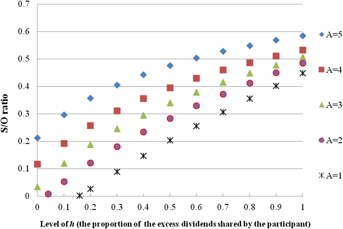
Figure 1. Relationship between the S/O ratio and the level of h
Table 4 assumes that h = 100% and the participant would spend a part of the additional cash on expenditures. To save space, we only report the effect that η (the proportion of the additional cash on expenditures) has on the S/O ratios when A = 2. If η = 0, the participant would spend none of the additional cash on expenditures, and the S/O ratios are the same as those in Table 2. There are two effects of η on the subjective value. From equation (5), we know that UnoG is the sum of
 $U(C_0 + \eta V)$
and
$U(C_0 + \eta V)$
and
 $e^{ - rT} U(W_T^V )$
. To satisfy equation (6), the term
$e^{ - rT} U(W_T^V )$
. To satisfy equation (6), the term
 $U(C_0 + \eta V)$
will make the subjective value negatively related to η, while the other term
$U(C_0 + \eta V)$
will make the subjective value negatively related to η, while the other term
 $e^{ - rT} U(W_T^V )$
implies that the subjective value will be positively associated with η. On the whole, Table 4 shows that the S/O ratios increase with η. As η increases, the participant would allocate less of the additional cash for investments when the pension does not have guaranteed interest credits, and it would be more difficult to accumulate enough wealth for retirement. These results reflect that the participant who prefers to consume now is more willing to have the guarantee mechanism and thus subjectively places a higher value on the guarantee. Similar implications hold in Table 5, where we set h = 0.
$e^{ - rT} U(W_T^V )$
implies that the subjective value will be positively associated with η. On the whole, Table 4 shows that the S/O ratios increase with η. As η increases, the participant would allocate less of the additional cash for investments when the pension does not have guaranteed interest credits, and it would be more difficult to accumulate enough wealth for retirement. These results reflect that the participant who prefers to consume now is more willing to have the guarantee mechanism and thus subjectively places a higher value on the guarantee. Similar implications hold in Table 5, where we set h = 0.
Table 4. Relationship between the S/O ratio and the level of η: A = 2, h = 100%, and a constant guarantee
Note: S/O is the ratio of the subjective value to the objective cost; η is the proportion of the additional cash amount on expenditures; h is the proportion of the excess dividends shared by the participant if the realized return on the pension portfolio exceeds the guaranteed return; A is the participant's relative risk aversion coefficient; ρ px is the correlation estimate between the returns on the pension portfolio and the risky tradable portfolio. At t = 0, all additional cash other than that spent on expenditures would be invested at the risk-free rate in case (i) or in the risky tradable portfolio in case (ii).
Table 5. Relationship between the S/O ratio and the level of η: A = 2, h = 0, and a constant guarantee
Note: S/O is the ratio of the subjective value to the objective cost; η is the proportion of the additional cash amount on expenditures; h is the proportion of the excess dividends shared by the participant if the realized return on the pension portfolio exceeds the guaranteed return; A is the participant's relative risk aversion coefficient; ρ px is the correlation estimate between the returns on the pension portfolio and the risky tradable portfolio. At t = 0, all additional cash other than that spent on expenditures would be invested at the risk-free rate in case (i) or in the risky tradable portfolio in case (ii). N/A means that a non-negative subjective value is not available.
Tables 2–5 report the S/O ratios with respect to three different pension portfolios. To lower the objective cost or the potential liabilities of the guarantee, the pension sponsor will direct contributions to investments with lower volatility, e.g., the pension portfolio with
 $\beta _p = 0.75$
and
$\beta _p = 0.75$
and
 $\sigma _p = 0.131$
. However, the pension sponsor may maximize the expected benefits from running the pension system or minimize the expected loss. For example, we define the sponsor's expected benefits or loss as
$\sigma _p = 0.131$
. However, the pension sponsor may maximize the expected benefits from running the pension system or minimize the expected loss. For example, we define the sponsor's expected benefits or loss as
 $E_0^P (\tilde W_T ),$
where
$E_0^P (\tilde W_T ),$
where
 $$\tilde W_T = (c_{er} + c_{ee} )W_0 \cdot (1 - h)\left( {\displaystyle{{S_{\,p,T}} \over {S_{\,p,0}}} - e^{gT}} \right)$$
if the realized return on the pension portfolio exceeds the guaranteed return; otherwise,
 $$\tilde W_T = (c_{er} + c_{ee} )W_0 \cdot \left( {\displaystyle{{S_{\,p,T}} \over {S_{\,p,0}}} - e^{gT}} \right).$$
We derive the expected benefits or loss in the real world using simple simulation techniques. The sponsor will choose
 $\beta _p = 1$
and
$\beta _p = 1$
and
 $\sigma _p = 0.16$
to minimize the expected loss if h = 100%, or
$\sigma _p = 0.16$
to minimize the expected loss if h = 100%, or
 $\beta _p = 1.71$
and
$\beta _p = 1.71$
and
 $\sigma _p = 0.32$
to maximize the expected benefits if h = 0.Footnote
10
As revealed in Tables 3 and 5, it is possible that a non-negative subjective value is unavailable when h = 0,
$\sigma _p = 0.32$
to maximize the expected benefits if h = 0.Footnote
10
As revealed in Tables 3 and 5, it is possible that a non-negative subjective value is unavailable when h = 0,
 $\beta _p = 1.71$
, and
$\beta _p = 1.71$
, and
 $\sigma _p = 0.32$
. This analysis suggests that the objective function of the pension sponsor will affect the subjective value and the S/O ratio.
$\sigma _p = 0.32$
. This analysis suggests that the objective function of the pension sponsor will affect the subjective value and the S/O ratio.
4 Extension: relative guarantee
When the guaranteed interest credit is a constant, we usually refer to it as an absolute guarantee. Comparably, a relative guarantee means that the guaranteed interest credit links to some non-constant indices. This section will analyze the subjective value of the relative guarantee.
Brown et al. (Reference Brown, Dybvig and Marshall2001) indicate that some credit rates of cash-balance pension systems link to a Treasury yield. We assume that the guaranteed interest credit links to the yield on Treasury bonds and use the Vasicek (Reference Vasicek1977) model to describe interest rates. The dynamics of short rates follow an Ornstein–Uhlenbeck process:
 $$dr_t^P = \kappa (b - r_t^P )dt + \sigma _r dB_{r,t}^P $$
and
 $$dr_t^Q = \kappa (b^{^\ast} - r_t^Q )dt + \sigma _r dB_{r,t}^Q, $$
where κ is the speed-of-adjustment coefficient and σ r is the dispersion coefficient of short rates. The mean-reversion level is b under the real-world P-measure and b* = b − σ r λ/κ under the risk-neutral Q-measure, where λ is the market price of risk. Equations (10) and (11), respectively, describe the short rates under the P- and Q-measures. Both of the measures are used in the following analysis because the participant subjectively places the value of the guarantee in the real world, but the objective cost of the guarantee is derived under the risk-neutral probability.
We substitute
 $\exp ( - \int_0^T {r_s^P ds} )$
for e
−rT
in equations (4) and (5), and the short rate can be expressed as
$\exp ( - \int_0^T {r_s^P ds} )$
for e
−rT
in equations (4) and (5), and the short rate can be expressed as
 $$r_{t + \Delta} ^P = r_t^P e^{ - \kappa \Delta} + b(1 - e^{ - \kappa \Delta} ) + \sigma _r \int\nolimits_t^{t + \Delta} {e^{ - \kappa (t + \Delta - s)}} dB_{r,s}^P $$
and
 $$r_{t + \Delta} ^Q = r_t^Q e^{ - \kappa \Delta} + b^{^\ast} (1 - e^{ - \kappa \Delta} ) + \sigma _r \int\nolimits_t^{t + \Delta} {e^{ - \kappa (t + \Delta - s)}} dB_{r,s}^Q. $$
The per-share price of the i-th asset is rewritten as:
 $$S_{i,t + \Delta} ^P = S_{i,t}^P \cdot \exp \left( {\int\nolimits_t^{t + \Delta} {r_s^P} ds + \left( {\beta _i \cdot EP - \displaystyle{1 \over 2}\sigma _i^2} \right)\Delta + \sigma _i B_{i,\Delta} ^P} \right)$$
and
 $$S_{i,t + \Delta}^{Q} = S_{i,t}^{Q} \cdot \exp \left( {\int\nolimits_t^{t + \Delta} r_{s}^{Q} ds - \displaystyle{1 \over 2}\sigma _i^2 \Delta + \sigma _i B_{i,\Delta}^{Q} } \right).$$
The θ-year spot rate at time t under the P-measure is
 $$\bar R^P (t,t + \theta ) = \displaystyle{{A(\theta ) + B(\theta ) \cdot r_t^P} \over \theta}, $$
where
 $$A(\theta ) = b(\theta - B(\theta )) - \displaystyle{{\sigma _r^2} \over {4\kappa ^3}} (4e^{ - \kappa \theta} - e^{ - 2\kappa \theta} + 2\kappa \theta - 3)$$
and
 $$B(\theta ) = \displaystyle{{1 - e^{ - \kappa \theta}} \over \kappa}. $$
We derive the spot rate in the real-neutral world with similar equations with
 $r_t^P $
and b replaced by
$r_t^P $
and b replaced by
 $r_t^Q $
and b*, respectively. The term (1 + r)
T
mentioned in Section 2 is replaced by
$r_t^Q $
and b*, respectively. The term (1 + r)
T
mentioned in Section 2 is replaced by
 $\prod\nolimits_{t = 0}^{T - 1} {(1 + \bar R^P (t,t + 1))} $
, implying that the participant allocates a portion of the wealth to a 1-year time deposit and renews it along with accrued interests at the end in each year. The guaranteed interest credit is defined as the average of the spot rates in the beginning of each year before retirement:
$\prod\nolimits_{t = 0}^{T - 1} {(1 + \bar R^P (t,t + 1))} $
, implying that the participant allocates a portion of the wealth to a 1-year time deposit and renews it along with accrued interests at the end in each year. The guaranteed interest credit is defined as the average of the spot rates in the beginning of each year before retirement:
 $$g = \displaystyle{{\sum\nolimits_{t = 0}^{T - 1} {\bar R(t,t + \theta )}} \over T},$$
where we use
 $\bar R^P $
when deriving the subjective value or
$\bar R^P $
when deriving the subjective value or
 $\bar R^Q $
when calculating the objective cost.
$\bar R^Q $
when calculating the objective cost.
We set θ = 30, i.e., the guaranteed return links to 30-year spot rates during the accumulation period. The initial short rate
 $r_0 $
is assumed to be 0.0163. We follow the parameter estimates in Hilliard and Hilliard (Reference Hilliard and Hilliard2015) to set κ = 0.3406, b = 0.0374, σ
r
= 0.0113, and σ
r
λ = −0.0028. For simplicity, the correlation estimate between the returns on the pension portfolio and the short rates (ρ
pr
) is −0.1 and that between the returns on the risky tradable portfolio and the short rates (ρ
xr
) is also −0.1. This setting implies that the returns on the pension portfolio and the risky tradable portfolio are likely to be positively correlated. Therefore, we only consider ρ
px
∈{0.2, 0.3, 0.4, 0.5} in this section.
$r_0 $
is assumed to be 0.0163. We follow the parameter estimates in Hilliard and Hilliard (Reference Hilliard and Hilliard2015) to set κ = 0.3406, b = 0.0374, σ
r
= 0.0113, and σ
r
λ = −0.0028. For simplicity, the correlation estimate between the returns on the pension portfolio and the short rates (ρ
pr
) is −0.1 and that between the returns on the risky tradable portfolio and the short rates (ρ
xr
) is also −0.1. This setting implies that the returns on the pension portfolio and the risky tradable portfolio are likely to be positively correlated. Therefore, we only consider ρ
px
∈{0.2, 0.3, 0.4, 0.5} in this section.
We simulate 100,000 paths using the method similar to that in the Appendix to obtain the subjective value of the relative guarantee. The standard Brownian motions under the P- and Q-measures are assumed to be independent of each other. The objective cost is also obtained by simulation because it is difficult to derive the closed-form formula for the objective cost under our assumptions about the relative guarantee. Table 6 reports the objective costs and the S/O ratios of our relative guarantee. In most cases, the subjective value is lower than the objective cost. The lower subjective value of the relative guarantee is because the participant will be anxious about the low realized guaranteed return when the guaranteed interest credit is linked to volatile interest rates. In the case where h = 0 and the pension portfolio is not very risky (or the pension portfolio is volatile but the level of risk aversion is low), the participant is more willing to exchange the guarantee for the upside potential benefits of the pension portfolio, and hence we cannot derive a non-negative subjective value of the guarantee. Table 7 assumes A = 2 and examines how the S/O ratio varies with the proportion of the additional cash on expenditures. Unlike the patterns in Tables 4 and 5, we find that the S/O ratio may decrease with η, especially when the pension portfolio is not volatile and the participant would allocate a part of additional cash amount to a 1-year time deposit. This finding points out that the participant may place a lower subjective value on the relative guarantee when he or she would consume more at present.
Table 6. S/O ratios with η = 0 and a relative guarantee

Note: S/O is the ratio of the subjective value to the objective cost; η is the proportion of the additional cash amount on expenditures; h is the proportion of the excess dividends shared by the participant if the realized return on the pension portfolio exceeds the guaranteed return; A is the participant's relative risk aversion coefficient. The minimum feasible ρ px (the correlation estimate between the returns on the pension portfolio and the risky tradable portfolio) is +0.2. At t = 0, all additional cash received in place of the guaranteed interest credit would be allocated to a 1-year time deposit in case (i) or be invested in the risky tradable portfolio in case (ii). N/A means that a non-negative subjective value is not available. S.E is the standard error of the objective cost.
Table 7. Relationship between the S/O ratio and the level of η: A = 2 and a relative guarantee
Note: S/O is the ratio of the subjective value to the objective cost; η is the proportion of the additional cash amount on expenditures; h is the proportion of the excess dividends shared by the participant if the realized return on the pension portfolio exceeds the guaranteed return; A is the participant's relative risk aversion coefficient. The minimum feasible ρ px (the correlation estimate between the returns on the pension portfolio and the risky tradable portfolio) is +0.2. At t = 0, all additional cash other than that spent on expenditures would be allocated to a 1-year time deposit in case (i) or in the risky tradable portfolio in case (ii). N/A means that a non-negative subjective value is not available. S.E is the standard error of the objective cost.
5 Conclusion
Though cash-balance pension plans have been adopted in many public sectors for at least a decade, they attract much less attention in academic literature than do defined-benefit or defined-contribution plans. This paper investigates how participants subjectively value the guarantee embedded in cash-balance pension plans. Because pension contracts embedded with guarantees cannot be traded in the market, participants cannot obtain the value of the guarantee from the market, and they may subjectively value the guarantee. We refer to and modify the framework of Hall and Murphy (Reference Hall and Murphy2000) to derive the subjective value perceived by participants.
The numerical results indicate that under many scenarios, participants place a lower subjective value on the guarantee than the objective cost derived through option pricing approaches. The subjective value may approach or even be below zero if the participant does not receive any excess dividends. A subjective value that is too low implies that the pension system potentially spends too much on the cash-balance plan embedded with a guarantee. However, we also find that, for some highly risk-averse participants, the subjective value will be higher than the objective cost. In sum, the subjective value depends on the level of risk aversion, the feasibility of diversification, the proportion of the excess dividends shared by the participant, the allocation of the additional cash amount received in place of the guaranteed return, the pension sponsor's objective function, etc. We suggest that, in addition to the objective cost, the pension system should estimate the subjective value of the guarantee when designing cash-balance plans lest the plan should be of extremely low value from the participant's perspective.
Further research could extend this paper in many ways. To clearly explain the concept of the subjective value, we do not include overly complicated model settings. However, it is worthwhile to consider the time-varying expected rates of return, volatilities, and asset correlations. The inclusion of inflation or mortality models is also worth considering. Additionally, practitioners and policy makers could evaluate subjective values of more guarantee structures and conduct a field survey to understand the subjective value of the guarantee determined by participants in the real world. Economists who are interested in the level of risk aversion in the pension market could adopt the framework of this paper and identify the level of risk aversion implicitly induced by the subjective value.
Appendix
Simulation procedures
This appendix explains how to derive the subjective value by simulation when the guaranteed interest credit rate is a constant. We could follow similar steps to obtain the subjective value of the relative guarantee.
Step A: For each mix of
 ${\rm (}\alpha, \beta _x, \sigma _x, \rho _{px} ),$
we simulate 100,000 paths of time-T prices of the risky tradable portfolio and the pension portfolio, and then we obtain the participant's total wealth at time T using equation (2) and utility with the guarantee using equation (4) along each path. The mean of the utility across the 100,000 paths is E
0 (U
G
). The maximum of these means is
${\rm (}\alpha, \beta _x, \sigma _x, \rho _{px} ),$
we simulate 100,000 paths of time-T prices of the risky tradable portfolio and the pension portfolio, and then we obtain the participant's total wealth at time T using equation (2) and utility with the guarantee using equation (4) along each path. The mean of the utility across the 100,000 paths is E
0 (U
G
). The maximum of these means is
 $\overline {EU} ^G $
.
$\overline {EU} ^G $
.
Step B: We substitute V = 0 into equations (3) and (5) and derive the mean of UnoG|
V=0 (the utility with V = 0 and without the guarantee) across all paths for each mix of
 $(\alpha, \beta _x, \sigma _x, \rho _{px} )$
. The mix of
$(\alpha, \beta _x, \sigma _x, \rho _{px} )$
. The mix of
 $(\tilde \alpha, \tilde \beta _x, \tilde \sigma _x, \tilde \rho _{px} )$
denotes the allocation that maximizes the mean of UnoG|
V=0.
$(\tilde \alpha, \tilde \beta _x, \tilde \sigma _x, \tilde \rho _{px} )$
denotes the allocation that maximizes the mean of UnoG|
V=0.
Step C1: We then derive the subjective value based on the allocation of
 $(\tilde \alpha, \tilde \beta _x, \tilde \sigma _x, \tilde \rho _{px} )$
.
$(\tilde \alpha, \tilde \beta _x, \tilde \sigma _x, \tilde \rho _{px} )$
.
-
(i) If the average of UnoG| V=0 is less than
 $\overline {EU} ^G $
, we repeatedly increase V by 100 until the average of UnoG is greater than
$\overline {EU} ^G $
. The first V such that the average of UnoG is greater than
$\overline {EU} ^G $
is denoted by UBV and regarded as the upper bound of the subjective value. In this step, the highest V such that the average of UnoG is lower than
$\overline {EU} ^G $
is denoted by LBV, which is the lower bound of the subjective value. We then proceed to Step C2.
$\overline {EU} ^G $
, we repeatedly increase V by 100 until the average of UnoG is greater than
$\overline {EU} ^G $
. The first V such that the average of UnoG is greater than
$\overline {EU} ^G $
is denoted by UBV and regarded as the upper bound of the subjective value. In this step, the highest V such that the average of UnoG is lower than
$\overline {EU} ^G $
is denoted by LBV, which is the lower bound of the subjective value. We then proceed to Step C2. -
(ii) If the average of UnoG| V=0 is higher than
$\overline {EU} ^G $
, we stop because under this scenario a non-negative subjective value is not available. -
(iii) If the average of UnoG| V=0 is equal to
$\overline {EU} ^G $
, we stop because we have obtained a non-negative subjective value.


Step C2: Substitute V = (LBV + UBV)/2 into equations (3) and (5).
-
(i) If the average of UnoG is higher than
$\overline {EU} ^G $
, we claim that the current V is too high and regard this V as the new UBV. We continue substituting V = (LBV + UBV)/2 into equations (3) and (5) until we find a new V such that the average of UnoG is lower than
$\overline {EU} ^G $
and regard this V as the new LBV. -
(ii) If the average of UnoG is lower than
$\overline {EU} ^G $
, we claim that the current V is still too low and regard this V as the new LBV. We continue substituting V = (LBV + UBV)/2 into equations (3) and (5) until we find the new UBV.


Step C3: Follow the concepts in Step C2 to repeatedly reset the UBV and LBV. The difference between the average of UnoG and
 $\overline {EU} ^G $
gradually shrinks. We stop when (i) the absolute difference between the average of UnoG and
$\overline {EU} ^G $
gradually shrinks. We stop when (i) the absolute difference between the average of UnoG and
 $\overline {EU} ^G $
is less than 10−10, and (ii) the absolute difference between the UBV and the LBV is less than 10−10. The subjective value is the final UBV or LBV, depending on which one generates an average of UnoG that is closer to
$\overline {EU} ^G $
is less than 10−10, and (ii) the absolute difference between the UBV and the LBV is less than 10−10. The subjective value is the final UBV or LBV, depending on which one generates an average of UnoG that is closer to
 $\overline {EU} ^G $
.
$\overline {EU} ^G $
.