


1. Introduction
Much attention has been paid to the investigation of particle-laden turbulence in recent decades. The behaviours of tracer and inertial particles in incompressible turbulence have been studied extensively, as for diffusion, collision and preferential concentration (Maxey Reference Maxey1987; Wang, Wexler & Zhou Reference Wang, Wexler and Zhou1998; Zhou, Wexler & Wang Reference Zhou, Wexler and Wang1998; Ott & Mann Reference Ott and Mann2000; Wilkinson, Mehlig & Bezuglyy Reference Wilkinson, Mehlig and Bezuglyy2006; Goto & Vassilicos Reference Goto and Vassilicos2008; Coleman & Vassilicos Reference Coleman and Vassilicos2009; Toschi & Bodenschatz Reference Toschi and Bodenschatz2009; Monchaux, Bourgoin & Cartellier Reference Monchaux, Bourgoin and Cartellier2012; Bourgoin & Xu Reference Bourgoin and Xu2014; Bragg, Ireland & Collins Reference Bragg, Ireland and Collins2015; Gustavsson & Mehlig Reference Gustavsson and Mehlig2016; Wang et al. Reference Wang, Wan, Yang, Wang and Chen2020). However, there has been much less study of compressible particle-laden turbulence, which is important for understanding flow in different domains – for example, scramjets (Ferri Reference Ferri1973; Curran, Heiser & Pratt Reference Curran, Heiser and Pratt1996; Huete et al. Reference Huete, Urzay, Sánchez and Williams2016; Urzay Reference Urzay2018) and the motion of interstellar gas (Barth & Rafkin Reference Barth and Rafkin2007; Johansen et al. Reference Johansen, Oishi, Mac Low, Klahr, Henning and Youdin2007; Pan et al. Reference Pan, Padoan, Scalo, Kritsuk and Norman2011). In this paper, we will focus mainly on the acceleration statistics of tracer and light particles dispersed in compressible homogeneous and isotropic turbulence (CHIT), an idealized set-up that could be helpful to the investigation on cavitating flow with clouds of bubbles (Reisman, Wang & Brennen Reference Reisman, Wang and Brennen1998; Wang & Brennen Reference Wang and Brennen1999; Fuster & Colonius Reference Fuster and Colonius2011).
Investigation of particle acceleration in turbulence has attracted much attention in the last 20 years. Following the ‘K41’ theory (Kolmogorov Reference Kolmogorov1941a,Reference Kolmogorovb), the Heisenberg–Yaglom model (Yaglom Reference Yaglom1949; Heisenberg Reference Heisenberg1985) was proposed to predict the variance of fluid acceleration in homogeneous isotropic turbulence (HIT):
 \begin{equation} \langle a^2 \rangle = a_0 \varepsilon^{3/2} \nu^{{-}1/2}, \end{equation}
where  $a$ is the acceleration magnitude,
  $\langle \cdot \rangle$ represents the ensemble average, and
  $a_0$ is a universal constant, which was further found to have an anomalous dependency on the Taylor microscale Reynolds number,
  $R_{\lambda }$, owing to the turbulent intermittency (Yeung & Pope Reference Yeung and Pope1989; Voth, Satyanarayan & Bodenschatz Reference Voth, Satyanarayan and Bodenschatz1998; Gotoh & Rogallo Reference Gotoh and Rogallo1999; Vedula & Yeung Reference Vedula and Yeung1999; Biferale et al. Reference Biferale, Boffetta, Celani, Devenish, Lanotte and Toschi2004). Also,
  $\varepsilon =2\nu \langle S_{ij}S_{ij} \rangle$ is the average dissipation rate,
  $S_{ij}$ is the rate-of-strain tensor, and
  $\nu$ is the kinematic viscosity. Yeung & Pope (Reference Yeung and Pope1989) found numerically that in HIT for fluid particles, the zero-crossing time (
 $\tau _0$, the time in which the autocorrelation function deceases to 0) of acceleration components is around
  $2.2$ times the Kolmogorov time scale (
 $\tau _{\eta }$). Moreover, the ratio of
  $\tau _0$ to
  $\tau _{\eta }$ barely varies with Reynolds number, which is supported by later investigations (Yeung Reference Yeung1997; Voth et al. Reference Voth, Satyanarayan and Bodenschatz1998; Mordant, Crawford & Bodenschatz Reference Mordant, Crawford and Bodenschatz2004; Biferale & Toschi Reference Biferale and Toschi2005; Volk et al. Reference Volk, Calzavarini, Verhille, Lohse, Mordant, Pinton and Toschi2008a). Subsequently, Yeung (Reference Yeung1997) discovered that
  $\tau _0$ of the acceleration magnitude is much larger than
  $\tau _{\eta }$. According to the momentum equation, the contribution to fluid acceleration can be decomposed into two parts: a pressure gradient term and a viscous force term. Vedula & Yeung (Reference Vedula and Yeung1999) pointed out that the contribution of the pressure gradient term is dominant over that of viscous force in turbulence. La Porta et al. (Reference La Porta, Voth, Crawford, Alexander and Bodenschatz2001) confirmed experimentally that the acceleration of fluid particles is extremely intermittent in fully developed turbulence. The probability density function (p.d.f.) of acceleration components is well reproduced by a superposition of stretched exponentials (Biferale et al. Reference Biferale, Boffetta, Celani, Devenish, Lanotte and Toschi2004), and the flatness factor of any component,
  $F_a = \langle (a_i)^4 \rangle / \langle (a_i)^2 \rangle ^2$, with
  $i=1,2,3$, can exceed 60 when
  $R_{\lambda }$ is up to 500. Later, many investigations on tracer particle acceleration in incompressible flows have been carried out (Voth et al. Reference Voth, La Porta, Crawford, Alexander and Bodenschatz2002; Mordant et al. Reference Mordant, Crawford and Bodenschatz2004; Xu et al. Reference Xu, Ouellette and Bodenschatz2007a,Reference Xu, Ouellette, Vincenzi and Bodenschatzb; Lavezzo et al. Reference Lavezzo, Soldati, Gerashchenko, Warhaft and Collins2010; Ni, Huang & Xia Reference Ni, Huang and Xia2012; Stelzenmuller et al. Reference Stelzenmuller, Polanco, Vignal, Vinkovic and Mordant2017).
Apart from tracer particles, the acceleration of inertial particles (both heavy and light particles) in incompressible turbulent flows also attracted much attention. Bec et al. (Reference Bec, Biferale, Boffetta, Celani, Cencini, Lanotte, Musacchio and Toschi2006) studied systematically the acceleration statistics of heavy particles in fully developed HIT. They pointed out that the flatness factor and the root-mean-square value of particle accelerations both sharply decrease with the increase of the Stokes number,  ${St} = \tau _p/\tau _\eta$, given by the ratio of particle response time and the Kolmogorov flow time. This is a combined effect of preferential concentration on regions with small pressure gradient and filtering due to inertia. Later, Ayyalasomayajula et al. (Reference Ayyalasomayajula, Gylfason, Collins, Bodenschatz and Warhaft2006) and Ayyalasomayajula, Warhaft & Collins (Reference Ayyalasomayajula, Warhaft and Collins2008) proposed a vortex model to describe the selective sampling of turbulent flows and filtering effects. On the contrary, it is known that in HIT, light particles enjoy the opposite behaviour, with a strong preferential concentration on high vorticity regions, and a p.d.f. of the acceleration even more intermittent than the tracer case and – in some cases – with shorter correlation times when normalized by
  $\tau _{\eta }$ (Volk et al. Reference Volk, Calzavarini, Verhille, Lohse, Mordant, Pinton and Toschi2008a,Reference Volk, Mordant, Verhille and Pintonb). Recently, Zhang, Legendre & Zamansky (Reference Zhang, Legendre and Zamansky2019) proposed a theoretical model that predicts successfully the variance of light particles acceleration with different density ratios when St is small (e.g. less than 1.0), as well as the dependence of drag force and inertia force on St.
In recent years, developments of experimental and numerical techniques also prompted a new interest in Lagrangian properties in compressible flows (Yang et al. Reference Yang, Wang, Shi, Xiao, He and Chen2013, Reference Yang, Wang, Shi, Xiao, He and Chen2014, Reference Yang, Wang, Shi, Xiao, He and Chen2016; Zhang et al. Reference Zhang, Liu, Ma and Xiao2016; Zhang & Xiao Reference Zhang and Xiao2018; Dai et al. Reference Dai, Luo, Jin and Fan2017, Reference Dai, Jin, Luo and Fan2018; Xiao et al. Reference Xiao, Jin, Luo, Dai and Fan2020). Yang et al. (Reference Yang, Wang, Shi, Xiao, He and Chen2013) investigated the accelerations of tracer particles in CHIT. They found that close to shocklets, the probability of extremely-large-acceleration events is increased. Moreover, almost all the large-acceleration events come from compression regions, and the autocorrelation function of acceleration components near shocklets decreases much faster than near vortices. Subsequently, Yang et al. (Reference Yang, Wang, Shi, Xiao, He and Chen2014) studied the influence of shocklets on inertial particles at  $M_t \approx 1.0$. They discovered that the p.d.f. of the longitudinal acceleration of light particles in compression regions has a much wider tail at the positive value than that of tracer and heavy particles. It results from the fact that light particles in compression regions have a higher probability to develop a velocity pointing upstream (the low-pressure side), compared with tracer and heavy particles. Recently, Haugen et al. (Reference Haugen, Brandenburg, Sandin and Mattsson2022) studied the clustering of heavy particles in two different compressible isotropic flows: compressively forced turbulence and solenoidally forced turbulence. They found that the clustering of particles in compressively forced turbulence peaks at two different St values. The first peak (at lower St) results from the contribution of shocklets, and the other is attributed to the centrifugal sling effect.
In this paper, we present a systematic investigation of bubble acceleration statistics at high Reynolds numbers and changing the degree of compressibility, i.e. the turbulent Mach number, and the results will be compared with those of tracer particles. In particular, we are interested in characterizing the role played by the presence of shocklets at changing  $M_t$ concerning both the single time p.d.f. of bubble acceleration and its temporal correlation. One of the main results is the identification of a critical Mach number
  $M_t \sim 0.6$ where the statistics of bubbles strongly departs from that of tracers.
The outline of the paper is as follows. The numerical details are introduced in § 2. The more important results and analysis are described in § 3. Finally, a brief conclusion and discussion is given in § 4.
2. Simulation configuration
Three-dimensional CHIT was simulated in a periodic cubic box with each side of length  $2{\rm \pi}$, based on a hybrid scheme (Wang et al. Reference Wang, Wang, Xiao, Shi and Chen2010) that combines the seventh-order weighted essentially non-oscillatory (WENO) scheme and eighth-order compact central finite difference scheme. The dimensionless governing equations of compressible turbulent flow are
 $$\begin{gather} \frac{\partial \rho_f}{\partial t}+\boldsymbol{\nabla} \boldsymbol{\cdot} \left(\rho_f \boldsymbol{u} \right) =0, \end{gather}$$
 $$\begin{gather}\frac{\partial \rho_f \boldsymbol{u}}{\partial t}+\boldsymbol{\nabla}\boldsymbol{\cdot}\left(\rho_f \boldsymbol{u} \boldsymbol{u}\right)={-}\boldsymbol{\nabla} \left(\frac{p}{\gamma M^2}\right)+\frac{1}{{Re}} \boldsymbol{\nabla}\boldsymbol{\cdot} \boldsymbol{\sigma} +\boldsymbol{f}, \end{gather}$$
 $$\begin{gather}\frac{\partial \varTheta}{\partial t}+\boldsymbol{\nabla}\boldsymbol{\cdot}\left[\left(\varTheta+\frac{p}{\gamma M^2}\right)\boldsymbol{u} \right] =\frac{1}{\alpha}\boldsymbol{\nabla}\boldsymbol{\cdot}\left(\kappa \boldsymbol{\nabla} T\right)+\frac{1}{{Re}}\boldsymbol{\nabla}\boldsymbol{\cdot}\left(\boldsymbol{\sigma}\boldsymbol{\cdot} \boldsymbol{u}\right) +\boldsymbol{f}\boldsymbol{\cdot}\boldsymbol{u}+\varLambda, \end{gather}$$
 $$\begin{gather}p=\rho_f T, \end{gather}$$
where  $\rho _f$,
  $\boldsymbol {u}$ and
  $p$ represent the density, velocity and static pressure of fluid, respectively, and
  $\gamma$ is the ratio of the specific heat at constant pressure,
  $C_p$, to the specific heat at constant volume,
  $C_v$. Here,
  $\boldsymbol {\sigma }=\mu [\boldsymbol {\nabla } \boldsymbol {u} + (\boldsymbol {\nabla } \boldsymbol {u})^{\rm T}]-\frac {2}{3}\mu \theta \boldsymbol {I}$ is the viscous stress, where
  $\mu$ is the dynamic viscosity,
  $\theta =\boldsymbol {\nabla }\boldsymbol {\cdot }\boldsymbol {u}$ is the divergence of fluid velocity, and
  $\boldsymbol {I}$ is the identity matrix. Also,
  $M=U_0/ c_0$ and
  ${Re}=\rho _0U_0L_0/ \mu _0$ are the reference Mach number and Reynolds number. Here,
  $L_0$,
  $\rho _0$,
  $U_0$,
  $\mu _0$ and
  $c_0$ are the reference length, density, velocity, dynamic viscosity and speed of sound, respectively,
  $\varTheta =p/[(\gamma -1)\gamma M^2]+\frac {1}{2}\rho _f\boldsymbol {u}\boldsymbol {\cdot }\boldsymbol {u}$ is the total energy per unit volume,
  $T$ denotes the temperature,and
  $\kappa$ is the thermal conductivity;
  $\alpha ={Pr}\,{Re} (\gamma -1)M^2$ is a coefficient from non-dimensionalization, where
  ${Pr}$ is the reference Prandtl number, which is specified as 0.7 in this paper. To maintain a stationary flow, an external force
  $\boldsymbol {f}$ is applied on the solenoidal velocity components at large scales (the first two wavenumbers). Furthermore, a uniform cooling term (
 $\varLambda$) is used to keep the internal energy steady. The detailed description of the forcing and cooling mechanism was introduced in Wang et al. (Reference Wang, Wang, Xiao, Shi and Chen2010), Federrath et al. (Reference Federrath, Roman-Duval, Klessen, Schmidt and Mac Low2010) and Kida & Orszag (Reference Kida and Orszag1990). In this paper, the turbulent Mach number (
 $M_t$) varies from 0.36 to 1.00, with Taylor Reynolds number
  $R_{\lambda } \approx 120$, and the total grid number (
 $N^3$) in the computational domain is
  $512^3$. Detailed parameters of the simulations are listed in table 1.
Table 1. Simulation parameters: Taylor Reynolds number  $R_{\lambda }$, turbulent Mach number
  $M_t$, grid points
  $N^3$, kinematic viscosity
  $\nu$, average dissipation rate of kinetic turbulent energy
  $\varepsilon$, Kolmogorov length scale
  $\eta$, Kolmogorov time scale
  $\tau _{\eta }$, root-mean-square fluctuation velocity
  $u_{rms}=\sqrt {\langle u_iu_i \rangle }$, integral length scale
  $L_f=\bigl (3{\rm \pi} /(2u_{rms}^2)\bigr ) \int _0^{+\infty } [E(k)/k]\,{\rm d}k$, and large-scale eddy turnover time
  $T_f=\sqrt {3}L_f/u_{rms}$;
  $E(k)$ denotes the kinetic energy at wavenumber
  $k$.
$k$.

The light particles are regarded as point objects, neglecting the influence of particles on turbulent flows and their mutual interaction. The motion of light particles is governed by
 $$\begin{gather} \frac{\mathrm{d}\kern0.06em \boldsymbol{x}_p}{\mathrm{d} t}=\boldsymbol{v}_p, \end{gather}$$
 $$\begin{gather}\frac{\mathrm{d}\boldsymbol{v}_p}{\mathrm{d}t}=\frac{\boldsymbol{u}_p-\boldsymbol{v}_p}{\tau_p} +\beta\,\frac{\mathrm{D}\boldsymbol{u}_p}{\mathrm{D}t} , \end{gather}$$
 $$\begin{gather}\tau_p=\frac{\rho_f d^2}{12\beta\mu}, \end{gather}$$
 $$\begin{gather}\beta=\frac{3\rho_f}{2\rho_p+\rho_f}, \end{gather}$$
where  $\boldsymbol {x}_p$,
  $\boldsymbol {v}_p$,
  $\tau _p$ and
  $d$ are the position, velocity, response time and diameter of particles, respectively, and
  $\boldsymbol {u}_p$ is the velocity of the flow at the position of the particle. Here,
  $\mu$ is the dynamic viscosity of fluid at the position of particles, and we notice that both
  $\tau$ and
  $\beta$ are dependent on space and time due to the variation of the underlying fluid density
  $\rho _f$. As a result, in a compressible flow, even a particle with density
  $\rho _p$ equal to the average flow density
  $\langle \rho _f \rangle$ will nevertheless be locally subjected to inertial forces due to the variation of the local flow density, where
  $\beta =1$ denotes the transition from particles heavier to lighter than the surrounding flow. In our case we have chosen
  $\rho _p = 0.01 \langle \rho _f \rangle$ for the light particles. It is important to stress that (2.6) must be considered an approximation of the true point-like description of inertial forces. Besides corrections present also in incompressible forces, as the Faxen and Basset terms (Maxey & Riley Reference Maxey and Riley1983; Gatignol Reference Gatignol1983), here we also need to consider new forces induced by density variations of the fluid flow at the particle positions (Parmar, Haselbacher & Balachandar Reference Parmar, Haselbacher and Balachandar2011, Reference Parmar, Haselbacher and Balachandar2012). In Appendix A we present a thoughtful discussion about these new effects and show that at moderate Mach numbers, such as the one investigated here, they can be safely neglected most of the time. The fluid velocity at the position of particles,
  $\boldsymbol {u}_p$, is evaluated by a fourth-order Lagrangian interpolation. The operator
  $\mathrm {D}/ \mathrm {D}t$ represents the material derivative. The number of particles that are uniformly released into the computational domain after the flow reaches a statistically steady state is
  $256^3$. After the particles are fully mixed, we sample over 15 times large-eddy turnover time (
 $T_f$) to explore the spatial, instantaneous statistics of particles. The Stokes number (
 ${St}=\tau _p/\tau _{\eta }$) of particles is approximately 0.21, and the average of
  $\beta$ is around 2.94. In addition, tracer particles whose velocity follows the local fluid velocity are analysed for comparison.
3. Results and analysis
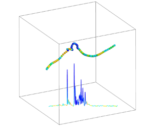
Before presenting the results from the statistical analysis, we show in figure 1 some characteristic evolution of the acceleration magnitudes,  $a$, along tracers and light particles trajectories near strong compression structures (e.g. shocklets) at
  $M_t=0.51$ and
  $M_t=1.00$, colour coded in terms of the local fluid compressibility
  $\theta$. For tracer particles, there is no significant difference between
  $M_t=0.51$ and 1.00, except for the larger peak of acceleration magnitudes near shocklets at
  $M_t=1.00$. For bubbles at
  $M_t=0.51$, the evolution of acceleration magnitudes is similar to that of tracer particles. However, at
  $M_t=1.00$, bubbles seem to be trapped near the shocklets for a long time (several times
  $\tau _{\eta }$), and the acceleration magnitudes of particles fluctuate dramatically. For the sake of completeness, the root-mean-square of acceleration magnitudes,
  $a_{rms}$, is shown in table 2. As one can see, as
  $M_t$ increases from 0.36 to 1.00,
  $a_{rms}$ of tracers increases slightly, whereas
  $a_{rms}$ of bubbles increases dramatically with increasing
  $M_t$, especially for
  $M_t > 0.64$. In addition, for light particles the root-mean-square values of the two terms in the right-hand side of (2.6) are also measured (not shown). The root-mean-square of the drag term is comparable to (slightly smaller than) that of the
  $\beta \,\mathrm {D}\boldsymbol {u}_p/ \mathrm {D}t$ term at all
  $M_t$.

Figure 1. The evolution of the acceleration magnitude,  $a$, of typical tracers (a,b) and light particles (c,d) at
  $M_t=0.51$ and
  $M_t=1.00$. The colourbar indicates the divergence of fluid velocity,
  $\theta$, at the position of particles. Here
  $a_{rms}$ and
  $\theta _{rms}$ represent the root- mean-square values of
  $a$ and
  $\theta$, respectively.
Table 2. Values for  $a_{rms}$ of tracers and bubbles at different
  $M_t$ values.

The p.d.f.s of one component of the particle accelerations,  $a_i$, with
  $i=1, 2, 3$, are illustrated in figure 2. It is apparent that all p.d.f.s have some intense stretched tails, indicating that the accelerations of tracer and bubbles are both intermittent. Unfortunately, the multifractal model used to predict successfully the p.d.f. of acceleration for tracers (Biferale et al. Reference Biferale, Boffetta, Celani, Devenish, Lanotte and Toschi2004) in incompressible flows cannot be translated easily to the case of inertial particles. This is due to the fact that it is not known how to correlate the local fluctuations of the Kolmogorov time with the effects of preferential concentration and filtering induced by the presence of inertia. Furthermore, the compressible effects add another direction that is not fully under control with the multifractal approach. The strength of intermittency can be quantified by the flatness of the acceleration component defined as
  $F_a = \langle (a_1)^4 \rangle / \langle (a_1)^2 \rangle ^2$, where here by
  $\langle \cdot \rangle$ we indicate the average among all particles. For tracers,
  $F_a$ increases steadily with the increase of
  $M_t$, as seen in figure 3. However,
  $F_a$ of light particles does not follow this trend. As
  $M_t$ increases from 0.36 to 1.00,
  $F_a$ of bubbles first increases, then reduces after
  $M_t$ exceeds about 0.6. The increase of
  $F_a$ of tracer particles (also applicable for bubbles at
  $M_t < 0.6$) is attributed to the fact that increasing compressibility increases the flow intermittency. However, when
  $M_t > 0.6$, why does
  $F_a$ of light particles decrease with the increase of
  $M_t$? Figure 4 shows the marginal cumulated distribution
  $P(a,\theta _m)=\int _{-\infty }^{\theta _m} P(a,\theta ) \,\mathrm {d}\theta$ of particle acceleration components conditioned to fall in different flow regions. We define CR1, CR2 and CR3 to represent the flow regions where
  $\theta _m < -\theta _{rms}$,
  $\theta _m < -2\theta _{rms}$ and
  $\theta _m < -3\theta _{rms}$ separately. For the sake of clarity, we mark the boundaries of CR1, CR2 and CR3 in figure 5 where the p.d.f.s of the divergence of fluid velocity at different
  $M_t$ are shown. Figure 4 reflects that the stretched tails of acceleration p.d.f.s result predominantly from the particles in strong compression regions when
  $M_t > 0.6$. In addition,
  $F_a$ is impacted heavily by the tails of acceleration p.d.f.s, as shown in the insets of figure 2. Therefore, we argue that the decrease of
  $F_a$ should be related to the statistical properties of bubbles in compression regions when
  $M_t>0.6$.

Figure 2. The p.d.f.s,  $P(a_{i})$, of one component of the accelerations
  $a_i$, normalized with its root-mean-square. Because of isotropy, all three components are equivalent. For clarity, here we show only the case with
  $i=1$. Panel (a) is for tracer particles. Inset:
  $(a_1)^4P(a_1)$ at
  $M_t=1.00$ is presented to check the statistical convergence of the fourth-order moments. Panel (b) is for light particles. Inset:
  $(a_1)^4P(a_1)$ is shown at
  $M_t=0.64$.

Figure 3. The flatness factor of particle acceleration components,  $F_a$, at changing
  $M_t$ for tracers (red squares) and light particles (blue diamonds). The error bar is calculated from the scatter among 30 subsamples obtained from 30 time snapshots.

Figure 4. The cumulated marginal p.d.f.s of particle acceleration components  $P(a,\theta _m)$, with
  $\theta _m=-\theta _{rms}$,
  $-2\theta _{rms}$ and
  $-3\theta _{rms}$ for CR1, CR2 and CR3, respectively. The black solid line is the reference p.d.f. obtained by considering the particles on the whole computational domain (
 $\theta _m=+\infty$). The red dotted, green dashed and blue dash-dotted lines are for CR1, CR2 and CR3, respectively. Panels (a–c) are for tracer particles at
  $M_t=0.51$, 0.64 and 1.00, respectively; (d–f) are for light particles at
  $M_t=0.51$, 0.64 and 1.00.

Figure 5. The p.d.f.s of the divergence of fluid velocity,  $\theta$, evaluated in the whole computational domain at
  $M_t=0.51$,
  $0.64$ and
  $1.00$. The three vertical lines separately mark the boundaries of CR1, CR2 and CR3, where
  $\theta < -\theta _{rms}$,
  $\theta < -2\theta _{rms}$ and
  $\theta < -3\theta _{rms}$.
Let us first compare  $F_a$ values of light particles in different regions, as shown in figure 6, where: case 1 represents the whole domain; case 2 represents the region with
  $\theta >-3\theta _{rms}$ (removing CR3 from case 1); case 3 represents the region with
  $\theta >-2\theta _{rms}$ (removing CR2 from case 1); case 4 represents the region with
  $\theta >-\theta _{rms}$ (removing CR1 from case 1). We can notice that at
  $M_t=0.64$,
  $F_a$ decreases sharply once the light particles in CR3 are removed. In contrast, at
  $M_t=1.00$,
  $F_a$ increases steadily as the particles in CR3, CR2 and CR1 are removed. Figure 7 also shows the p.d.f.s of
  $a_1$ of light particles at cases 1, 2, 3 and 4 when
  $M_t = 0.64$ and
  $1.00$. The tails of the p.d.f.s of
  $a_1$ for
  $M_t = 0.64$ become much narrower when the light particles in strong compression regions are removed, whereas the tails, at
  $M_t = 1.00$, become wider since the light particles in CR3, CR2 and CR1 are removed. To explain this difference, in figure 8, we compare the number of bubbles and tracers in CR3. Here, we can see that the number of tracers keeps a quite low level when
  $M_t \in [0.36, 1.00]$ although it is slightly increasing. On the other hand, the number of bubbles in CR3 increases dramatically when
  $M_t>0.6$, especially at
  $M_t=1.00$, accounting for approximately
  $25\,\%$ of the total particle number in the whole domain. That is, bubbles will accumulate significantly in strong compression regions (near shocklets). Figure 9 shows the distribution of light particles and
  $\theta$ in a quasi-two-dimensional slice with
  $M_t = 0.64$ and
  $1.00$. As one can see, bubbles tend to accumulate in strong compression regions at
  $M_t = 1.00$, which is different to what happens at
  $M_t = 0.64$. In order to understand the preferential concentration, it is key to control the divergence of particles’ velocities as derived from (2.6), and assuming that
  $\beta$ and
  $\tau _p$ do not vary significantly with space and time, we have
 \begin{equation} \boldsymbol{\nabla}\boldsymbol{\cdot}\boldsymbol{v}_p \approx \theta + \tau_p(1-\beta)\left(Q-\frac{\mathrm{D}\theta}{\mathrm{D}t}\right). \end{equation}
Here,  $Q=\varOmega _{ij}\varOmega _{ij}-S_{ij}S_{ij}$ is the second-order invariant of fluid velocity gradients, where
  $\varOmega _{ij}$ and
  $S_{ij}$ are the rate-of-rotation tensor and rate-of-strain tensor, respectively, and
  $\mathrm {D}\theta / \mathrm {D}t = \partial \theta / \partial t + \boldsymbol {u}\boldsymbol {\cdot } \boldsymbol {\nabla } \theta$ is the material derivative of
  $\theta$. From (3.1) one can see that light particles (
 $\beta >1$) tend to accumulate in the regions
  $\theta <0$,
  $Q>0$ and
  $\mathrm {D}\theta / \mathrm {D}t<0$. From the above expression, it is clear that the prediction on preferential concentration for the case of inertial particles in compressible flows is much more complicated than in the incompressible case, being connected to cross-correlations among compressibility of the carrying flow, inertia parameters and local flow topology. In order to achieve a systematic understanding of such a complex phenomenon, one would need refined scanning at changing of
  $\tau _p$ and
  $\beta$ parameters too, which is outside the scope of this paper.

Figure 6.  $F_a$ of light particles in different regions: case 1, the whole domain; case 2, the regions with
  $\theta > -3\theta _{rms}$ (removing CR3 from case 1); case 3, the regions with
  $\theta > -2\theta _{rms}$ (removing CR2 from case 1); case 4, the regions with
  $\theta > -\theta _{rms}$ (removing CR1 from case 1).

Figure 7. The p.d.f.s of  $a_1$ of light particles in different regions when
  $M_t=0.64$ (a) and
  $M_t=1.00$ (b).

Figure 8. The ratio of the particle number in CR3 to the total particle number in the whole domain.

Figure 9. The distribution of light particles and  $\theta$ in a two-dimensional slice when
  $M_t=0.64$ (a) and
  $M_t=1.00$ (b). Here, all particles lie in a quasi-two-dimensional slice with a width in the third dimension of the order of the Kolmogorov length scale. X and Y represent the x-coordinate and y-coordinate of slices.
According to figure 4, one can understand that the particles with extremely large accelerations come predominantly from the strong compression regions (such as CR3) at high  $M_t$. Then, if the number of particles in CR3 is small (like tracers), the probability of the particles with large accelerations is still small. Therefore, a slight increase of particle number in CR3 will make a contribution to the enhancement of the acceleration intermittency. Hence
  $F_a$ of tracers increases with the increase of
  $M_t$. On the other hand, if the number of particles in CR3 is large, as for the case of bubbles at
  $M_t = 0.77 - 1.00$, there will be a large portion of particles with large accelerations, which can no longer be regarded as rare events. Then the increase of particle number in CR3 will no longer contribute to the increase of acceleration intermittency. As a result, the preferential concentration of bubbles in strong compression regions (e.g. CR3) results in the decrease of
  $F_a$ when
  $M_t > 0.6$. In order to further validate this mechanism, the flatness factor of acceleration components of fluid elements at the position of bubbles,
  $F_a^u$, is measured, shown in figure 10 where
  $F_a^u$ varies with the same trend as
  $F_a$ of light particles. Therefore, we confirm that the decrease of
  $F_a$ of light particles at
  $M_t > 0.6$ is attributed to the preferential concentration of light particles in strong compression regions.

Figure 10. The flatness factor of acceleration components of fluid elements at the position of light particles,  $F_a^u$, versus
  $M_t$.
It is also worth explaining why  $F_a$ of light particles increases dramatically at
  $M_t\in [0.5,0.6]$. One understands that the particles in CR3 (near shocklets) have large accelerations in general. Figure 8 shows that the number of tracers in CR3 always keeps a quite low level, and it slightly increases as
  $M_t$ increases from 0.36 to 1.00, resulting in a significant increase of the intermittency of acceleration. Therefore,
  $F_a$ of tracers increases steadily with increasing
  $M_t$. The number of bubbles is also low when
  $M_t < 0.6$, but it increases faster than the number of tracers at
  $M_t\in [0.5,0.6]$, so that the number of light particles in CR3 at
  $M_t=0.64$ has been up to that of tracers at
  $M_t = 1.00$, leading to a fast increase of
  $F_a$.
3.1. Longitudinal acceleration at different  $M_t$
$M_t$

The longitudinal acceleration,  $a_L=(\boldsymbol {a}\boldsymbol {\cdot }\boldsymbol {v}_p)/ |\boldsymbol {v}_p|$, is the projection of acceleration (
 $\boldsymbol {a}$) to the direction of particle velocity (
 $\boldsymbol {v}_p$), which determines how fast the magnitude of velocity varies. Figure 11 presents the p.d.f.s of
  $a_L$ of particles at
  $M_t = 0.36 - 1.00$. One can see that for tracers, the p.d.f.s of
  $\boldsymbol {a}_L$ are skewed towards negative values. However, for bubbles, the p.d.f.s of
  $\boldsymbol {a}_L$ skew only moderately to the negative value at low
  $M_t$ (e.g.
  $M_t=0.51$), and this trend vanishes as the p.d.f.s become almost symmetric at high
  $M_t$ (e.g.
  $M_t=1.00$). To quantify this difference, we measure the skewness factor of
  $\boldsymbol {a}_L$,
  $S_a$, as shown in figure 12. For tracers,
  $S_a$ becomes more negative as
  $M_t$ increases from 0.36 to 1.0. As is well known, shocklets will appear in compression regions with the increase of
  $M_t$. When tracer particles pass through the shocklets from upstream to downstream, they will be decelerated significantly owing to the negative pressure gradient (Anderson Reference Anderson2010). As
  $M_t$ increases, the shocklets become stronger (the deceleration is also more remarkable). Therefore, the p.d.f. of
  $\boldsymbol {a}_L$ is more skewed to negative values and
  $S_a$ becomes more negative for tracers when
  $M_t$ increases.

Figure 11. The p.d.f.s of longitudinal accelerations for (a) tracer particles, (b) light particles.

Figure 12. The skewness factor of particle longitudinal accelerations,  $S_a$, varies with
  $M_t$.
As shown in figure 12, for light particles,  $S_a$ also decreases with
  $M_t$ when
  $M_t$ is small, similar to the situation for tracers. However,
  $S_a$ gradually goes back to zero after
  $M_t > 0.6$. A similar phenomenon was suggested by Yang et al. (Reference Yang, Wang, Shi, Xiao, He and Chen2014), who discovered that
  $S_a$ of light particles in compression regions is close to 0 at
  $M_t \approx 1.03$, and there are many light particles whose velocities have an obtuse angle with local pressure gradient. To understand the above difference between tracers and bubbles, we show in figure 13 the p.d.f. of
  $\cos \alpha$ in CR1 (compression region with
  $\theta <-\theta _{rms}$), where
  $\alpha$ is the angle between the velocity of particles and the local pressure gradient. One can see that most tracers in CR1 have angle
  $\alpha <90^{\circ }$ (
 $\cos \alpha >0$) at all
  $M_t$. However, for light particles, the number of particles with
  $\alpha >90^{\circ }$ (
 $\cos \alpha <0$) increases steadily as
  $M_t$ increases from 0.6 to 1.0 approximately. Then we measure how many particles have angle
  $\alpha < 90^{\circ }$ before entering CR1, denoted as
  $N_{CR1}^{in}$, and once inside CR1, denoted as
  $N_{CR1}$. Figure 14 shows that for tracer particles,
  $N_{CR1}$ is always close to
  $N_{CR1}^{in}$ at different
  $M_t$. That is, tracers rarely change their direction in CR1. However, for light particles,
  $N_{CR1}$ is noticeably smaller than
  $N_{CR1}^{in}$ at high
  $M_t$, and this deviation becomes more significant as
  $M_t$ increases. That is, as
  $M_t$ increases, more bubbles reverse their direction of velocity from
  $\alpha < 90^{\circ }$ to
  $\alpha > 90^{\circ }$ in CR1, so that more light particles that were decelerated turn to be accelerated. This is the main reason for the p.d.f. of
  $\boldsymbol {a}_L$ being more symmetric when
  $M_t>0.6$. Also,
  $N_{CR1}$ of light particles decreases moderately as
  $M_t$ increases from 0.6 to 1.0, which implies that at high
  $M_t$, more light particles have positive longitudinal accelerations when they are entering CR1.

Figure 13. The p.d.f.s of  $\cos \alpha$ in CR1. Here,
  $\alpha$ is the angle between the velocity of particles and the local pressure gradient: (a) tracer particles; (b) light particles.

Figure 14. The ratios of  $N_{{CR1}}^{in}$ (red squares) and
  $N_{{CR1}}$ (blue diamonds) to the total number of particles in CR1. The empty symbols are for tracers, and the filled symbols are for light particles. Here,
  $N_{{CR1}}^{in}$ denotes the number of particles with
  $\alpha <90^{\circ }$ when entering CR1, and
  $N_{{CR1}}$ denotes the number of particles with an angle of
  $\alpha <90^{\circ }$ in CR1.
Why do many light particles reverse their velocity direction from  $\alpha < 90^{\circ }$ to
  $\alpha > 90^{\circ }$ in CR1, but few tracers do? As one can see from (2.6), the effect of local fluid acceleration on light particles is amplified by
  $\beta$ (
 $\beta \approx 2.94$ in our simulations). Thus it is easier to decelerate light particles by the negative pressure gradient near shocklets, compared with tracers. Assuming that a tracer and a light particle enter the shocklets from upstream at the same time, both will be decelerated under the negative pressure gradient. In general, the tracer particle can pass through the shocklets successfully. However, the velocity of the light particle could decrease to zero, or even have its direction reversed since
  $\beta$ amplifies the effect of negative pressure gradient. For example, the comparison between
  $N_{{CR1}}^{in}$ and
  $N_{{CR1}}$ in figure 14 reflects quantitatively that at
  $M_t=1.00$,
  $51\,\%$ of light particles in CR1 reverse their velocity direction from
  $\alpha < 90^{\circ }$ to
  $\alpha > 90^{\circ }$, but few tracer particles do.
3.2. Autocorrelation function of acceleration components at different $M_t$

Figure 15 shows the autocorrelation function of the first component of accelerations  $R_1(\tau )=\langle a_1(t)\,a_1(t+\tau ) \rangle / \langle a_1(t)^2 \rangle$ (because of isotropy,
  $R_2$ and
  $R_3$ would be equal to
  $R_1$). One can notice that in the small time scale, the
  $R_1$ values for tracers and bubbles both decrease faster for increasing
  $M_t$. However, for tracers, the zero-crossing time,
  $\tau _0$, barely varies with
  $M_t$, and it is approximately close to
  $2.3\tau _{\eta }$, which is similar to the results in incompressible turbulence (Yeung Reference Yeung1997; Mordant et al. Reference Mordant, Crawford and Bodenschatz2004; Volk et al. Reference Volk, Calzavarini, Verhille, Lohse, Mordant, Pinton and Toschi2008a). For bubbles,
  $\tau _0$ is also approximately equal to
  $2.3\tau _{\eta }$ when
  $M_t<0.6$. In fact, it is slightly smaller than the value for tracer particles, as shown in figure 16. Volk et al. (Reference Volk, Calzavarini, Verhille, Lohse, Mordant, Pinton and Toschi2008a) found that
  $\tau _0$ of light particles in incompressible homogeneous isotropic turbulence is significantly smaller than the value for tracers, which is slightly different from our results. This might be attributed to the fact that
  ${St}=1.64$ in the work by Volk et al. (Reference Volk, Calzavarini, Verhille, Lohse, Mordant, Pinton and Toschi2008a), whereas
  ${St}\approx 0.2$ in our simulations. Also shown in figure 16 is that when
  $M_t>0.6$,
  $\tau _0$ of light particles will gradually decrease with the increase of
  $M_t$, unlike the value for tracer particles.

Figure 15. The autocorrelation function,  $R_1(\tau )$, of
  $a_1$ at different
  $M_t$, for (a) tracers, (b) light particles.

Figure 16.  $\tau _0$ varies with
  $M_t$ for tracers (red squares) and light particles (blue diamonds).
Why is the trend of the changes of  $\tau _0$ between tracer and light particles different from each other at high
  $M_t$? Yang et al. (Reference Yang, Wang, Shi, Xiao, He and Chen2013) found that the autocorrelation function of acceleration of tracers near shocklets decreases much faster than that near vortices in CHIT. In addition, we use the persistence time
  $\tau _c$ to denote the period needed for the particles to pass across the strong compression regions (CR3), as shown in figure 17(a). It is found that the average of
  $\tau _c$ among tracers,
  $\langle \tau _c \rangle$, is smaller than
  $\tau _{\eta }$, and it decreases slightly with the increase of
  $M_t$ (
 $\langle \tau _c \rangle \approx 0.2\tau _{\eta }$ at
  $M_t = 1.00$), as shown in figure 17(b). For light particles,
  $\langle \tau _c \rangle$ is similar to that for tracer particles when
  $M_t < 0.6$. However, as
  $M_t$ increases further,
  $\langle \tau _c \rangle$ increases dramatically, up to around 4
 $\tau _{\eta }$ at high
  $M_t$. Then one can argue that
  $R_1(\tau )$ of tracers is barely influenced by shocklets since the time that tracers stay in strong compression regions is quite short. Therefore,
  $\tau _0\approx 2.34\tau _{\eta }$ of tracers is independent of
  $M_t$ and close to the value of the small-scale eddy turnover time. For light particles, at low
  $M_t$ (e.g.
  $M_t=0.51$),
  $\langle \tau _c \rangle$ is similar to that for tracers so that
  $\tau _0$ of bubbles is quite close to that of tracers. However, as
  $M_t$ increases,
  $\langle \tau _c \rangle$ of light particles increases gradually because more bubbles will be trapped in strong compression regions (near shocklets) for several
  $\tau _{\eta }$, as shown in figure 18(b), where the p.d.f.s of
  $\tau _c$ of light particles present two peaks when
  $M_t > 0.6$, which is different to what happens for tracers; see figure 18(a). The position of the first peak (
 $\tau _c / \tau _{\eta }=0.2 - 0.3$) is similar to that of tracers. However, the second peak occurs in the range of
  $\tau _c / \tau _{\eta }=3.0 - 4.0$, indicating that many bubbles are trapped by shocklets, hence the influence on
  $R_1(\tau )$ becomes remarkable, and
  $\tau _0$ of light particles decreases with increasing
  $M_t$. In order to confirm the above conclusion further, we have measured
  $R_1(\tau )$ for light particles when the events of
  $\tau _c > 1.0$ are removed at
  $M_t=1.00$, as shown in figure 19. As expected,
  $R_1(\tau )$ for light particles decreases much more slowly when the events of
  $\tau _c > 1.0$ are removed, and
  $\tau _0$ increases by approximately five times. Therefore, we confirm the observation that the decrease of
  $\tau _0$ with increasing
  $M_t$ is attributed to the larger number of light particles that are trapped near shocklets for a long time.

Figure 17. (a) The history curve of  $\theta$ along one trajectory of bubble at
  $M_t=1.00$. Here,
  $\tau _c$ denotes the time over which particles pass through CR3. (b) The average value of characteristic time of particles staying in CR3,
  $\langle \tau _c \rangle$, at different
  $M_t$.

Figure 18. The p.d.f.s of the time ( $\tau _c$) that particles stay in strong compression regions (CR3) at different
  $M_t$, for (a) tracers, (b) light particles.

Figure 19. For light particles,  $R_1(\tau )$ at
  $M_t = 1.00$ after the events of
  $\tau _c > 1.0$ are removed (blue squares) compared with the unconditioned case (red circles).
It is also worth noting the oscillation of  $R_1(\tau )$ for light particles at high
  $M_t$, as shown in figure 15(b). From the preceding analysis, bubbles could be trapped in vortices and near shocklets for comparable time scales. We believe that the strong oscillatory behaviour is the combined effect of both vortices and shocklets, as confirmed by plotting the conditioned autocorrelation function in figure 19, where the oscillation disappears when the events of
  $\tau _c > 1.0$ have been removed.
4. Conclusion and discussion
The acceleration statistics of tracer and light particles (bubbles) in CHIT have been studied. Our main finding is related to the characteristic signature of the presence of shocklets in the probability density function of acceleration and on its characteristic correlation times. In particular, we found that at  $M_t \sim 0.6$, the statistical properties of bubble acceleration start to be strongly different from those of the underlying tracers, developing a sort of condensation on and near shocklet structures, where a high percentage of the total number of particles is concentrated. As a consequence, acceleration flatness, skewness and autocorrelation time are strongly affected. We find that in the range investigated here,
  $M_t \in [0.31,1]$ the flatness factor of acceleration components,
  $F_a$, of tracers increases monotonically with
  $M_t$. For light particles,
  $F_a$ also increases with
  $M_t$ at
  $M_t< 0.6$. However, when
  $M_t>0.6$,
  $F_a$ of bubbles decreases with
  $M_t$ because of preferential accumulation in strong compression regions.
The p.d.f.s of the longitudinal acceleration of tracers are found to be skewed towards negative values, and as  $M_t$ increases, the skewness factor,
  $S_a$, becomes more negative. For light particles,
  $S_a$ also becomes more negative with the increase of
  $M_t$, followed by a tendency to return to 0 after
  $M_t > 0.6$. We attribute the tendency of the longitudinal acceleration p.d.f. of light particles to become more and more symmetric at high
  $M_t$ to the fact that more particles reverse their direction of velocity from
  $\alpha < 90^{\circ }$ to
  $\alpha > 90^{\circ }$ in compression regions (e.g. regions with
  $\theta < -\theta _{rms}$) at increasing compressibility, together with the fact that more bubbles with positive longitudinal acceleration enter compression regions at higher
  $M_t$.
We have found that for tracers, the characteristic persistence time,  $\tau _c$, near shocklets is quite short, especially at high
  $M_t$ (
 $\langle \tau _c \rangle \approx 0.2\tau _{\eta }$ at
  $M_t=1.00$). Hence the autocorrelation function of acceleration components,
  $R_1(\tau )$, decreases faster at higher
  $M_t$ in the small time scale, while the zero-crossing time,
  $\tau _0$, does not vary too much with
  $M_t$. For light particles, as
  $M_t$ increases, larger number of particles are trapped near shocklets for several
  $\tau _{\eta }$, so the influence of shocklets on the autocorrelation function of accelerations becomes remarkable. Therefore,
  $\tau _0$ is influenced greatly by shocklets and decreases with
  $M_t$.
The results in this paper are obtained under the point-particle approximation, supposing that the radius of tracers and bubbles is not larger than the Kolmogorov length scale ( $\eta$). Furthermore, it is important to make sure also that the typical width of shocklets is not too small, in order to not break the validity of the above assumption. In our direct numerical simulations, even the stronger shocklets have a size within
  $2\eta \sim 3 \eta$, keeping the approximation reasonably valid.
The strong singular signature of shocklets for the dynamics and statistics of light particles opens up many important questions that need further numerical and experimental studies. In particular, the role of correction terms in (2.6) induced by the presence of compressibility must be better elucidated, as discussed in Appendix A. Second, in the presence of strong particles’ concentration near shocklets, the importance of bubble–bubble collision, breakup and coalescence should be quantified better, as well as their feedback on the flow. Finally, future work also needs to provide detailed studies of preferential concentration properties when changing both the Stokes time and added mass parameters, in order to have more comprehensive control of the behaviour of inertial particles at changing Mach number.
Funding
We are grateful to Professor J. Wang for providing the DNS code for CHIT. This work is funded by the National Numerical Wind Tunnel Project (no. NNW2019ZT1-A01), the National Natural Science Foundation of China (grant no. 91752201), the Department of Science and Technology of Guangdong Province (grant no. 2019B21203001), the Key Special Project for Introduced Talents Team of Southern Marine Science and Engineering Guangdong Laboratory (Guangzhou) (grant no. GML2019ZD0103), and the Shenzhen Science and Technology Innovation Committee (grant no. KQTD20180411143441009). We acknowledge computing support provided by the Center for Computational Science and Engineering of the Southern University of Science and Technology. L.B. acknowledges hospitality from the Southern University of Science and Technology and funding from the European Research Council (ERC) under the European Unions Horizon 2020 research and innovation programme (grant agreement no. 882340).
Declaration of interests
The authors report no conflict of interest.
Appendix A
According to Parmar et al. (Reference Parmar, Haselbacher and Balachandar2012), the governing equation for the movement of light particles in compressible turbulence can be expressed (neglecting history force) as
 $$\begin{gather} \rho_p \frac{\mathrm{d} \boldsymbol{v}_p}{\mathrm{d} t}=\frac{9\mu}{2a^2} \left(\boldsymbol{u}_p-\boldsymbol{v}_p \right)+\rho_f\frac{\mathrm{D} \boldsymbol{u}_p}{\mathrm{D} t}+\frac{1}{2}\left[\frac{\mathrm{D} \left(\rho_f \boldsymbol{u}_p \right)}{\mathrm{D} t}-\frac{\mathrm{d} \left(\rho_f \boldsymbol{v}_p \right)}{\mathrm{d} t}\right], \end{gather}$$
 $$\begin{gather}\frac{\mathrm{d} \boldsymbol{v}_p}{\mathrm{d} t}=\frac{\boldsymbol{u}_p-\boldsymbol{v}_p}{\tau_p}+\beta\frac{\mathrm{D} \boldsymbol{u}_p}{\mathrm{D} t} +\frac{\beta}{3\rho_f}\left[\boldsymbol{u}_p\frac{\mathrm{D} \rho_f}{\mathrm{D} t}-\boldsymbol{v}_p\frac{\mathrm{d} \rho_f}{\mathrm{d} t}\right]. \end{gather}$$
From the mass conservation equation, we have
 $$\begin{gather} \frac{\mathrm{D}\rho_f}{\mathrm{D}t}={-}\rho_f \boldsymbol{\nabla} \boldsymbol{\cdot} \boldsymbol{u}, \end{gather}$$
 $$\begin{gather}\frac{\mathrm{d}\rho_f}{\mathrm{d}t}=\frac{\mathrm{D}\rho_f}{\mathrm{D}t} +\left(\boldsymbol{v}_p-\boldsymbol{u}_p \right)\boldsymbol{\cdot} \boldsymbol{\nabla} \rho_f. \end{gather}$$
Substituting (A3) and (A4) into (A2), we get
 \begin{equation} \frac{\mathrm{d} \boldsymbol{v}_p}{\mathrm{d} t}=\frac{\boldsymbol{u}_p-\boldsymbol{v}_p}{\tau_p}+\beta\frac{\mathrm{D} \boldsymbol{u}_p}{\mathrm{D}t}+\left\{ \frac{\beta}{3}\left(\boldsymbol{v}_p-\boldsymbol{u}_p\right)\boldsymbol{\nabla} \boldsymbol{\cdot} \boldsymbol{u}_p-\frac{\beta}{3\rho_f}\boldsymbol{v}_p\left[\left(\boldsymbol{v}_p -\boldsymbol{u}_p\right) \boldsymbol{\cdot} \boldsymbol{\nabla} \rho_f\right]\right\} . \end{equation}
 If St is small ( $\tau _p$ is quite small), then (
 $\boldsymbol {v}_p-\boldsymbol {u}_p$) in the third term on the right-hand side of (A5) will also be small as
  $\boldsymbol {v}_p=\boldsymbol {u}_p+O(\tau _p)$. However, in compressible flows,
  $\boldsymbol {\nabla } \boldsymbol {\cdot } \boldsymbol {u}_p$ and
  $\boldsymbol {\nabla } \rho _f$ will increase as
  $M_t$ increases. Consequently, there is a question of whether the contribution of the third term on the right-hand side of (A5) can be neglected. Here, we define
 \begin{equation} \left.\begin{gathered} {F_1}=\left|\frac{\boldsymbol{u}_p-\boldsymbol{v}_p}{\tau_p}\right|,\\ {F_2}=\left|\beta\frac{\mathrm{D} \boldsymbol{u}_p}{\mathrm{D}t}\right|,\\ {F_3}=\left|\frac{\beta}{3}\left(\boldsymbol{v}_p-\boldsymbol{u}_p\right) \boldsymbol{\nabla} \boldsymbol{\cdot}\boldsymbol{u}_p-\frac{\beta}{3\rho_f}\boldsymbol{v}_p \left[\left(\boldsymbol{v}_p-\boldsymbol{u}_p\right)\boldsymbol{\cdot}\boldsymbol{\nabla}\rho_f\right]\right|, \end{gathered}\right\} \end{equation}
and then measure the averages of  ${F_1}$,
  ${F_2}$ and
  ${F_3}$ among all particles at different time slices, in order to have an a priori estimate of the importance of the neglected terms. In figure 20, we show that the contribution of
  $\mathrm {F_3}$ is well below
  $5\,\%$ up to
  $M_t=0.6$, and becomes of the order of 10–15 % only at the largest Mach number,
  $M_t=1.00$. As a result, we argue that the approximation that we made is reasonably acceptable up to the largest Mach number that we have investigated, and we leave for future studies the question of checking the precise impact of the extra terms in (A5) for those Mach regimes.

Figure 20. The average values of  ${F_1}$,
  ${F_2}$ and
  ${F_3}$ among all particles at different time slices.


