


1. Introduction
The snake arm maintainer (SAM) is a type of hyper-redundant robot [Reference Chirikjian and Burdick1,Reference Runciman, Darzi and Mylonas2,Reference Bing, Zang, Chen, Wang, Lang, Zhu, Yang and Yi3] with a simplified structure enabled by placing the driver unit (e.g., the motor) outside the workspace of the robot [Reference Palmer4]. The robot’s motion posture can then adopt a relatively complete, streamlined configuration [Reference Nemitz, Mihaylov, Barraclough, Ross and Stokes5]. In such an externally driven “bionic tendon” design, the drive system is concentrated at the rear, that is, in the tail of the snake arm, and the entire arm length is free of electronic equipment. Therefore, it is suitable for high-risk, radiation-containing, narrow-space operations such as those conducted in nuclear power plants [Reference Buckingham and Graham6]. The China Fusion Engineering Test Reactor (CFETR) is an international scientific project aimed at solving the energy problem caused by human demand. The safe and stable operation of a test reactor is inseparable from the regular monitoring and maintenance of the remote handling system [Reference Song, Wu, Wan, Li, Ye, Zheng, Yong, Zhao and Wei7]. Traditional industrial robots cannot be deployed in narrow, multi-obstacle, radiation-containing vacuum chamber environments. In contrast, SAMs demonstrate excellent environmental adaptability and obstacle avoidance; moreover, their encirclement mechanism allows work in unstructured and multi-device environments [Reference Armada, Buckingham and Graham8]. Therefore, SAMs are expected in the monitoring and maintenance of large and complex equipment in narrow spaces.
Inspired by snake movements, OC Robotics designed a bionic snake arm that maneuvers in extreme environments [Reference Buckingham9]. This design adopts the principles of under-actuated hyper-redundant robots and wire rope traction. A snake arm comprises several basic joints (flexible rods, springs, or multi-joint arms with universal joints) connected in series [Reference Ming, Agheli and Onal10,Reference Li, Liu, Liu and Leng11,Reference He, Liu, Wang and Hua12]. Each basic unit runs along a set joint trajectory to reach the end point P of the snake arm. By following the target curve, the snake arm completes its specified task. The snake arm can be retracted by winding on a spiral column [Reference Palmer and Axinte13,Reference Dong, Axinte, Palmer, Cobos, Raffles, Rabani and Kell14]. Bending curves in the kinematics modeling of the snake arm can be described through differential geometry, and the forward kinematics can be implemented by a modified Denavit–Hartenberg program [Reference Hannan and Walker15]. The traditional generalized inverse matrix method is unsuitable for solving the inverse kinematics and trajectory planning of snake arms, because a snake arm includes many joints and degrees of freedom [Reference Seraji16–Reference Omisore, Han, Ren, Zhang and Lei18]. With recent computational developments, the inverse kinematics of hyper-redundant robots can be solved by neural network methods and various genetic algorithms [Reference Xidias19,Reference Yin, Wang and Yang20]. However, as these methods require a long learning time, they cannot fulfill real-time needs. Using a geometric method called space inverse kinematics, Samer et al. set equal angles of adjacent joints and identified a set of definite solutions to avoid joint singularity [Reference Yahya, Moghavvemi and Mohamed21]. Chirikjian proposed the backbone curve method to solve the inverse kinematics of hyper-redundant robots [Reference Chirikjian and Burdick22] and [Reference Chirikjian and Burdick23]. This method fits the segmented backbone curve of the snake arm to the backbone curve describing the arm’s macroscopic configuration. Common backbone methods include the pattern function backbone method [Reference Fahimi, Ashrafiuon and Nataraj24,Reference Fahimi, Ashrafiuon and Nataraj25] and the Bessel backbone method [Reference Song, Li, Meng, Yu and Ren26]. Xu et al. achieved obstacle avoidance by grouping the key points of the snake arm and refitting them to the backbone curve [Reference Xu, Mu, Liu and Liang27]. In traditional hyper-redundant robots, the number of kinematic executable degrees of freedom exceeds the freedom of the robot’s workspace [Reference Mu, Yu, an, Xu, Liu and Liang28]. This situation requires a large drive and control system which enlarges the volume and weight. Continuous robots can exhibit multiple degrees of freedom but not all of them are directly driven [Reference Langer, Amanov and Burgner29,Reference Talas, Baydere and Altinsoy30]. Although the number of motors is reduced in a continuous robot, the tension force problem remains, meaning that the precision degrades at the end of a long cantilever with a large load [Reference William and Walker31].
In order to meet the actual requirements of CFETR on the load and volume of SAM, this study proposes a new SAM for operation in the narrow working space of the vacuum chamber of CFETR. The new snake arm is designed with a layered structure, which reduces the number of driving motors and increases the arm length and space curvature. The inverse kinematics and trajectory planning of the snake arm are solved using the backbone curve method. By setting inverse solution conditions, SAM obstacle avoidance and inverse solution optimization are realized. The trajectory tracking motion control of the snake arm is realized by the variable rod length algorithm. The driving signals of the wire rope are solved by matrix transformation and distance equation. In addition, the SAM prototype (arm length 2300 m) experiments are used to verify the rationality of the layered drive and the correctness of the motion control methods.
The rest of this article is arranged as follows: Section 2 describes the structural principle of the layer-driven SAM. Section 3 describes the trajectory planning and trajectory tracking motion control algorithms of the layer-driven SAM. The motion control experiments and their results are presented in Section 4. Finally, a short conclusion is drawn in Section 5.
2. An under-Actuated SAM for Nuclear Power Plants
2.1. SAM model design
The layered driven SAM is an under-actuated robot with hyper-redundancy. This design is suitable for high-precision manipulation of large loads, and simplifies the drive box. A typical SAM consists of three parts: a multi-joint snake arm, a drive box, and a moving platform (see Fig. 1(a)). The layered driven design method drives multiple joints with a single three-motor driving layer.

Figure 1. Snake arm maintenance system. (a) SAM machine model and (b) vacuum chamber at the CFETR.
The designed SAM is mounted on a large heavy-duty mechanical arm (Fig. 1(b)), and is used for visual detection, flaw detection, dust removal, and other tasks in the vacuum chamber of the nuclear power plant, which constitutes a complex multi-obstacle environment. This paper mainly discusses the structure and control design of the snake arm and drive box. The layered driving principle is designed for the actual operating environment of nuclear power plants. The arm consists of 10 joints, each of diameter 80 mm and length 200 mm. According to the comprehensive performance of the degree of freedom, joint diameter, and load, SAM is divided into four joint groups with a number ratio of 3:3:2:2. Figure 2(a) shows the configuration of each rigid joint in the joint group. Fifteen rows of wire rope fed through holes are arranged along the circumference of each joint, and a sufficient support force is ensured by a support plate installed between each row of through holes. The rigid joints are connected by universal joints, as shown in Fig. 2(b). Besides allowing many motional degrees of freedom, the designed under-actuated SAM possesses the load capacity and control precision of a hyper-redundant robot, enabling its application in nuclear power plants and other extreme environments.
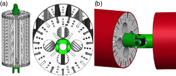
Figure 2. Details of the snake arm structure. (a) Joint configuration and (b) universal joint connecting two joints.
Principle of the layered drive structure: each joint group of the SAM is designed following the layered drive principle. Suppose that the i-th joint group contains three rigid joints, as shown in Fig. 3. The drive cables of this joint group pass along three rows of wire rope threaded through holes with an angular separation of 120
 $^{\circ}$
along the circumference, as shown in Fig. 3(a). The wire ropes are layered and fixed at the first, second, and third joints from outside to inside, as shown in Fig. 3(b). The drive box is installed with a servo motor and composite capstan (Fig. 4) that synchronize the angular movements of the rigid joints (Fig. 3(b)). The composite capstan pulls a row of wire ropes from top to bottom. Ignoring the slight position error from the cable through hole to the joint axis, the diameter of each winding groove of the composite capstan can be designed according to the ratio of
$^{\circ}$
along the circumference, as shown in Fig. 3(a). The wire ropes are layered and fixed at the first, second, and third joints from outside to inside, as shown in Fig. 3(b). The drive box is installed with a servo motor and composite capstan (Fig. 4) that synchronize the angular movements of the rigid joints (Fig. 3(b)). The composite capstan pulls a row of wire ropes from top to bottom. Ignoring the slight position error from the cable through hole to the joint axis, the diameter of each winding groove of the composite capstan can be designed according to the ratio of
 $1:2:3$
from top to bottom.
$1:2:3$
from top to bottom.

Figure 3. Principle of the layered drive structure. (a) Joint cross section and (b) a single joint group (with three rigid joints).
The advantages of the layer-driven SAM are as follows. First, the number of driving motors and the volume of the driving box are greatly reduced compared with the hyper-redundant robot to realize the lightweight and miniaturized design. Second, the position accuracy and load capacity are higher than those of a continuous robot, and an accurate kinematic model can be established for motion control. Third, the control system and the inverse motion solution are simplified while maintaining a high curvature.
Table I. DH parameter table of SAM.


Figure 4. SAM drive box and the composite capstan.

Figure 5. SAM link coordinate system.
2.2. SAM kinematics modeling
SAM kinematics describes the relationship between the motion of each joint and the relative motion of each link. For the SAM composed of multiple universal joints in series, the direction of motion of each adjacent joint is orthogonal, and the kinematics model is relatively simple. Based on the SAM prototype model, the coordinate system shown in Fig. 5 is established to describe the motion relationship of each joint, and the Denavit–Hartenberg (D−H) parameters are established as shown in Table I. The homogeneous transformation matrix of the basic coordinate system
 ${A_0}$
on the drive box is as follows:
${A_0}$
on the drive box is as follows:
 \begin{align}{D_0} = Trace\left( {a,b,{{c}}} \right)Trace\left( {0,u,0} \right) = \left[ \begin{array}{c@{\quad}c@{\quad}c@{\quad}c} 1 & 0 &0& a \\ 0 &1 &0 &{u + b} \\ 0 &0 &1 &c \\ 0 &0 &0 &1 \\ \end{array} \right]\end{align}
where
 $\left[ {a,b,c} \right]$
is the position of point
$\left[ {a,b,c} \right]$
is the position of point
 ${B_0}$
in the coordinate system of point
${B_0}$
in the coordinate system of point
 ${A_0}\left( {{x_0},{y_0},{z_0}} \right)$
.
${A_0}\left( {{x_0},{y_0},{z_0}} \right)$
.
 $u$
is the y-axis feed displacement. The homogeneous transformation matrix between any adjacent links
$u$
is the y-axis feed displacement. The homogeneous transformation matrix between any adjacent links
 ${U_i}$
in joint group 1 is:
${U_i}$
in joint group 1 is:
 \begin{align} {D_i^{i - 1} = Trace\left( {0,{l_i},0} \right)Rot\left( {{z_{2i}},{\alpha _1}} \right)Rot\left( {{y_{2i}},{\pi \over 2}} \right)Rot\left( {{z_{2i + 1}},{\beta _1}} \right)Rot\left( {{y_{2i + 1}}, - {\pi \over 2}} \right)} \nonumber\\[3pt] = \left[ \begin{array}{c@{\quad}c@{\quad}c@{\quad}c}{{\rm{c}}{\alpha _1}} &{ - {\rm{s}}{\alpha _1}c{\beta _1}} &{{\rm{s}}{\alpha _1}s{\beta _1}} &0 \\ {{\rm{s}}{\alpha _1}} &{{\rm{c}}{\alpha _1}c{\beta _1}} &{ - {\rm{c}}{\alpha _1}s{\beta _1}} &{{l_i}} \\ 0 &{s{\beta _1}} &{c{\beta _1}} &0 \\ 0& 0 &0 &1 \\ \end{array} \right] \,\end{align}
where
 ${l_i}$
is the length of the connecting rod;
${l_i}$
is the length of the connecting rod;
 ${\alpha _1},{\beta _1}$
are the joint angles of joint group 1, c denotes cos and s denotes sin. This convention will be adopted in future studies as well. From this, the relationship between the SAM end point coordinate system and the base coordinate system at
${\alpha _1},{\beta _1}$
are the joint angles of joint group 1, c denotes cos and s denotes sin. This convention will be adopted in future studies as well. From this, the relationship between the SAM end point coordinate system and the base coordinate system at
 ${A_0}$
can be obtained as:
${A_0}$
can be obtained as:
 \begin{align}{D_{10}} = {D_0}D_1^0D_2^1 \cdots D_{10}^9\end{align}
3. Motion Control Methods
3.1. Trajectory planning using improved backbone method
3.1.1. Backbone method kinematics modeling
According to the Frenet–Serret formula, any point
 $\textbf{W}\left( {x,t} \right)$
on curve
$\textbf{W}\left( {x,t} \right)$
on curve
 $\textbf{W}$
can be described by three linearly independent unit vectors
$\textbf{W}$
can be described by three linearly independent unit vectors
 $ {\boldsymbol\alpha \left( {x,t} \right),\boldsymbol\beta \left( {x,t} \right),\boldsymbol\gamma \left( {x,t} \right)}$
. These vectors form the basic three-prismatic shape of the curve, expressed as
$ {\boldsymbol\alpha \left( {x,t} \right),\boldsymbol\beta \left( {x,t} \right),\boldsymbol\gamma \left( {x,t} \right)}$
. These vectors form the basic three-prismatic shape of the curve, expressed as
 $\left\{ {\boldsymbol\alpha \left( {x,t} \right),\boldsymbol\beta \left( {x,t} \right),\boldsymbol\gamma \left( {x,t} \right)} \right\}$
with
$\left\{ {\boldsymbol\alpha \left( {x,t} \right),\boldsymbol\beta \left( {x,t} \right),\boldsymbol\gamma \left( {x,t} \right)} \right\}$
with
 \begin{align}\boldsymbol\alpha \left( {x,t} \right) = \dot{\textbf{W}}\left( {x,t} \right)\end{align}
 \begin{align}\boldsymbol\beta \left( {x,t} \right) = \frac{1}{\kappa }\dot{\boldsymbol\alpha} \left( {x,t} \right)\end{align}
 \begin{align}\boldsymbol\gamma \left( {x,t} \right) = \boldsymbol\alpha \left( {x,t} \right) \times \boldsymbol\beta \left( {x,t} \right)\end{align}
As shown in Fig. 6(a),
 $\boldsymbol\alpha \left( {x,t} \right)$
is the unit tangent vector of curve at point x, and the other vectors are perpendicular to
$\boldsymbol\alpha \left( {x,t} \right)$
is the unit tangent vector of curve at point x, and the other vectors are perpendicular to
 $\alpha \left( {x,t} \right)$
.
$\alpha \left( {x,t} \right)$
.
 $\kappa = \left| {\dot{\boldsymbol\alpha} \left( {x,t} \right)} \right|$
is the curvature of curve
$\kappa = \left| {\dot{\boldsymbol\alpha} \left( {x,t} \right)} \right|$
is the curvature of curve
 $\textbf{W}$
at point x.
$\textbf{W}$
at point x.

Figure 6. Coordinate system in the backbone method. (a) Definition of tangent line at any point on the backbone curve and (b) definition of the tangent line space pose of the backbone curve.
To preserve the important features of the backbone curve
 $\textbf{W}$
, we indirectly represent the arbitrary curves in three dimensions by solving the integral or differential equations. The integral form is given by
$\textbf{W}$
, we indirectly represent the arbitrary curves in three dimensions by solving the integral or differential equations. The integral form is given by
 \begin{align}\textbf{W}(x,t) = \mathop \smallint \limits_0^x l(\omega ,t){\boldsymbol{\alpha }}(\omega ,t)d\omega ,\end{align}
where
 $l\left( {x,t} \right)$
is the rate of change of arc length, which represents the tangent length of the curve (see Fig. 6(b)). The curve described by Eq. (7) can be interpreted as follows: starting from zero, change the forward direction along the tangent vector
$l\left( {x,t} \right)$
is the rate of change of arc length, which represents the tangent length of the curve (see Fig. 6(b)). The curve described by Eq. (7) can be interpreted as follows: starting from zero, change the forward direction along the tangent vector
 $\boldsymbol\alpha \left( {x,t} \right)$
and extend the curve along the new direction. Note that
$\boldsymbol\alpha \left( {x,t} \right)$
and extend the curve along the new direction. Note that
 $l\left( {x,t} \right)$
determines the speed of the extension. For a fixed-length curve,
$l\left( {x,t} \right)$
determines the speed of the extension. For a fixed-length curve,
 $l(x,t)=1$
.
$l(x,t)=1$
.
According to the parameterized curve defined by Eqs. (4), (5), and (7), the position of any point on the backbone curve can be expressed as
 \begin{align}\textbf{W}(x,t) = \left( \begin{array}{c} {\mathop \smallint \limits_0^x l(\omega ,t){\rm{sin}}\textbf{K}(\omega ,t){\rm{cos}}\textbf{T}(\omega ,t)d\omega } \\ \\[-9pt] {\mathop \smallint \limits_0^x l(\omega ,t){\rm{cos}}\textbf{K}(\omega ,t){\rm{cos}}\textbf{T}(\omega ,t)d\omega } \\ \\[-9pt] {\mathop \smallint \limits_0^x l(\omega ,t){\rm{sin}}\textbf{T}(\omega ,t)d\omega {\rm{}}} \\ \end{array} \right),\end{align}
where
 $\textbf{K}\left( {\omega ,t} \right)$
and
$\textbf{K}\left( {\omega ,t} \right)$
and
 $\textbf{T}\left( {\omega ,t} \right)$
indicate the direction of the tangent vector of the curve at point x at time t (see Fig. 6(b)), and
$\textbf{T}\left( {\omega ,t} \right)$
indicate the direction of the tangent vector of the curve at point x at time t (see Fig. 6(b)), and
 $l\left( {\omega ,t} \right)$
represents the length of the tangent vector. Therefore, the backbone curve can be parameterized by the three parameters
$l\left( {\omega ,t} \right)$
represents the length of the tangent vector. Therefore, the backbone curve can be parameterized by the three parameters
 $\left\{ {l,\textbf{K}},\textbf{T} \right\}$
, and the shape function of the specified task can be obtained by limiting and changing the pattern set comprising the abovementioned three functions
$\left\{ {l,\textbf{K}},\textbf{T} \right\}$
, and the shape function of the specified task can be obtained by limiting and changing the pattern set comprising the abovementioned three functions
 $\left\{ {l,\textbf{K}},\textbf{T} \right\}$
.
$\left\{ {l,\textbf{K}},\textbf{T} \right\}$
.
3.1.2. Inverse kinematics optimization algorithm
The forward kinematics of the backbone curve of the designed SAM can be obtained by numerically integrating Eq. (8), but the inverse kinematics problem has an infinite number of solutions. By limiting
 $\textbf{K}\left( {x,t} \right)\!,\textbf{T}\left( {x,t} \right)$
to a modal form, the inverse kinematics problem of SAM simplifies to
$\textbf{K}\left( {x,t} \right)\!,\textbf{T}\left( {x,t} \right)$
to a modal form, the inverse kinematics problem of SAM simplifies to
 \begin{align}K\left( {x,t} \right) = \mathop \sum \limits_{i = 1}^{{N_K}} {a_i}\left( t \right){\varphi _i}\left( x \right)\end{align}
 \begin{align}T\left( {x,t} \right) = \mathop \sum \limits_{i = {N_K} + 1}^{{N_T} + {N_K}} {a_i}\left( t \right){\varphi _i}\left( x \right)\end{align}
Here,
 ${a_i}\left( t \right)$
is the modal participation factor,
${a_i}\left( t \right)$
is the modal participation factor,
 ${\varphi _i}\left( x \right)$
is the modal function, and
${\varphi _i}\left( x \right)$
is the modal function, and
 ${N_K}$
and
${N_K}$
and
 ${N_T}$
are the number of modes distributed in the shape functions
${N_T}$
are the number of modes distributed in the shape functions
 $K\left( {x,t} \right)$
 ${\rm{and}}$
 $T\left( {x,t} \right)$
, respectively. Note that the total number of modes is
$T\left( {x,t} \right)$
, respectively. Note that the total number of modes is
 ${N_T} + {N_K}$
. The number of modal functions must be greater than or equal to the required number of geometric constraints of SAM. In this study, SAM is structurally incapable of expansion, so
${N_T} + {N_K}$
. The number of modal functions must be greater than or equal to the required number of geometric constraints of SAM. In this study, SAM is structurally incapable of expansion, so
 $l\left( {x,t} \right) = 1$
and no modal conversion is required.
$l\left( {x,t} \right) = 1$
and no modal conversion is required.
For a convenient calculation, the number of modal functions should be smaller than the number of degrees of freedom of SAM. The shape of the backbone curve for a given set of modal functions is completely limited by
 $\left\{ {{a_i}} \right\}$
. In this case, the inverse kinematics problem of SAM simplifies to the process of finding
$\left\{ {{a_i}} \right\}$
. In this case, the inverse kinematics problem of SAM simplifies to the process of finding
 $\left\{ {{a_i}} \right\}$
, which satisfies the spatial geometric position constraint of SAM.
$\left\{ {{a_i}} \right\}$
, which satisfies the spatial geometric position constraint of SAM.
The inverse kinematics can be obtained by solving the spatial kinematics of a closed-form SAM. For example, suppose that the backbone curve
 $l\left( {x,t} \right) = 1$
has
$l\left( {x,t} \right) = 1$
has
 ${N_T} = {N_K} = 2$
. Then, the backbone curve parameters of the SAM are
${N_T} = {N_K} = 2$
. Then, the backbone curve parameters of the SAM are
 $\textbf{K}\left( {x,t} \right){\rm{and}}\textbf{T}\left( {x,t} \right)$
, and the modal form in the rate state is set as
$\textbf{K}\left( {x,t} \right){\rm{and}}\textbf{T}\left( {x,t} \right)$
, and the modal form in the rate state is set as
 \begin{align}\dot{\textbf{K}}\left( {x,t} \right) = 2\pi {a_1}\cos \left( {2\pi x} \right) + 2\pi {a_2}\sin \left( {2\pi x} \right)\end{align}
 \begin{align}\dot{\textbf{T}}\left( {x,t} \right) = 2\pi {a_3}\cos \left( {2\pi x} \right) + 2\pi {a_4}\sin \left( {2\pi x} \right)\end{align}
where
 $\dot{\textbf{K}}\left( {x,t} \right){\rm{and}}\ \dot{\textbf{T}}\left( {x,t} \right)$
are the angular velocities of
$\dot{\textbf{K}}\left( {x,t} \right){\rm{and}}\ \dot{\textbf{T}}\left( {x,t} \right)$
are the angular velocities of
 $K\left( {x,t} \right){\rm{and}}\ T\left( {x,t} \right)$
, respectively, and the total number of modes is four. From Eqs. (11) and (12), we obtain
$K\left( {x,t} \right){\rm{and}}\ T\left( {x,t} \right)$
, respectively, and the total number of modes is four. From Eqs. (11) and (12), we obtain
 \begin{align}\textbf{K}\left( {x,t} \right) = \mathop \smallint \nolimits_0^x l\left( {\omega ,t} \right)\dot K\left( {\omega ,t} \right)d\omega = {a_1}\sin \left( {2\pi x} \right) - {a_2}\cos \left( {2\pi x} \right) + {a_2}\end{align}
 \begin{align}\textbf{T}\left( {x,t} \right) = \mathop \smallint \nolimits_0^x l\left( {\omega ,t} \right)\dot T\left( {\omega ,t} \right)d\omega = {a_3}\sin \left( {2\pi x} \right) - {a_4}\cos \left( {2\pi x} \right) + {a_4}\end{align}
Using the Bessel function [Reference Bowman32] and the identity transformation, and substituting Eqs. (13) and (14) into Eq. (8), the terminal coordinates of the backbone curve
 $\textbf{W}\left( {x,t} \right)$
are obtained as
$\textbf{W}\left( {x,t} \right)$
are obtained as
 \begin{align} {x_w} &= {1 \over 2}{J_0}\left[ {{{\left( {{{\left( {{a_1} + {a_3}} \right)}^2} + {{\left( {{a_2} + {a_4}} \right)}^2}} \right)}^{{1 \over 2}}}} \right]\sin \left( {{a_2} + {a_4}} \right) \nonumber\\[3pt]&\quad + {1 \over 2}{J_0}\left[ {{{\left( {{{\left( {{a_1} - {a_3}} \right)}^2} + {{\left( {{a_2} - {a_4}} \right)}^2}} \right)}^{{1 \over 2}}}} \right]\sin \left( {{a_2} - {a_4}} \right) \nonumber\\[3pt] {y_w} &= {1 \over 2}{J_0}\left[ {{{\left( {{{\left( {{a_1} + {a_3}} \right)}^2} + {{\left( {{a_2} + {a_4}} \right)}^2}} \right)}^{{1 \over 2}}}} \right]\sin \left( {{a_2} + {a_4}} \right) \nonumber\\[3pt] &\quad + {1 \over 2}{J_0}\left[ {{{\left( {{{\left( {{a_1} - {a_3}} \right)}^2} + {{\left( {{a_2} - {a_4}} \right)}^2}} \right)}^{{1 \over 2}}}} \right]\sin \left( {{a_2} - {a_4}} \right) \nonumber\\[3pt] {z_w} &= {J_0}\left[ {{{\left( {{{\left( {{a_3}} \right)}^2} + {{\left( {{a_4}} \right)}^2}} \right)}^{{1 \over 2}}}} \right]\sin \left( {{a_4}} \right) \end{align}
where
 ${J_0}$
is the Bessel function of order 0:
${J_0}$
is the Bessel function of order 0:
 \begin{align}{J_0}\left( x \right) = 1 - {\left( {\frac{1}{2}x} \right)^2} + \frac{{{{\left( {\frac{1}{2}x} \right)}^4}}}{{{1^2}\cdot{2^2}}} - \frac{{{{\left( {\frac{1}{2}x} \right)}^6}}}{{{1^2}{2^2}{3^2}}} + \cdots \cdots \end{align}
Eq. (15) is derived in the Appendix. The SAM is limited to four degrees of freedom. The end-effector position given by Eq. (15) has infinitely many solutions. The extra degrees of freedom can be used to modify the internal geometry of the backbone curve for obstacle avoidance and other operations.

Figure 7. Fitting the backbone curve of the SAM.
As an example, we solve the inverse kinematics on a SAM prototype with four joint groups (see Fig. 1). To solve the inverse kinematics in each joint of SAM, the discrete SAM trunk can be fitted to the continuous backbone curve. Here, the backbone curve was directionally fitted from the drive box to the end effector. To ensure a precisely reached target point, the inverse kinematics are solved by separating the end joint groups from the backbone curve. The end effector of the SAM is fixed to the end of the backbone curve, and the trunk is fitted to the backbone curve as far as possible for discretizing the backbone curve. The inverse kinematics of SAM are then obtained by inverse-solving the pose of each joint fitting the backbone curve of SAM.
The process of fitting the backbone curve differs between SAM and a hyper-redundant robot. SAM can fit only the start and end points of the joint group onto the backbone curve, causing errors in the actual poses of the joint groups and the theoretically calculated backbone curve (see Fig. 7); moreover, there is a risk of obstacle collisions. To optimize the inverse solution matching, the following principles are introduced. First is the principle of fitting the backbone curve. During the forward fitting process from driver box to end effector, the key points are matched and the inverse kinematics are solved for each joint group. To capture the geometric features and avoid obstacles, the penultimate key point near the end effector is separated from the backbone curve (yellow point in Fig. 7). The inverse kinematics are then solved with precise positioning of the end point. The second principle is the obstacle avoidance principle: when solving the inverse kinematics, each joint node of the SAM must be safely distanced from the center of an obstacle. Any inverse solution that violates the distance condition is abandoned (key points can be separated from the backbone curve in special cases). The third principle stipulates the minimum energy consumption and maximum stability. The inverse solution must ensure that each joint group rotates in the same direction as far as possible with the minimum rotational displacement. This principle obtains the trajectory with the minimum energy consumption and highest stability. The search process of the inverse solution optimization algorithm is shown in Fig. 8.

Figure 8. Flowchart of the inverse solution optimization algorithm for the SAM.
Before optimizing the inverse solution, the SAM coordinate system must be established. The coordinate system can be established at the start and end points of each joint group (Fig. 9(a)), or at each joint (Fig. 9(b)). To easily calculate the angle variation in each joint and the elongation of the wire ropes, the key points of the backbone curve are fitted in the first coordinate system, and the wire rope elongation is solved in the second coordinate system. The coordinate transformation in Fig. 9(a) is executed as follows:
 \begin{align}Trans\left( {{x_i},{y_i},{z_i}} \right) = \left[ \begin{array}{c@{\quad}c@{\quad}c@{\quad}c}1&0&0&{{a_i}}\\ \\[-7pt]0&1&0 &{{b_i}}\\\\[-7pt] 0 &0&1&{{c_i}}\\\\[-7pt]0&0&0&1\\\\[-7pt] \end{array} \right]\end{align}
 \begin{align}R\left( {x,3{\beta _i}} \right) = \left[ {\begin{array}{c@{\quad}c@{\quad}c@{\quad}c}1&0&0&0\\\\[-7pt]0&{c3{\beta _i}}& - s3{\beta _i}&0\\\\[-7pt] 0 &0& {s3{\beta _i}} & 0\\\\[-7pt] 0&0&0&1\\\\[-7pt] \end{array}} \right]\end{align}
 \begin{align}R\left( {y,{\alpha _i}} \right) = \left[ \begin{array}{c@{\quad}c@{\quad}c@{\quad}c}{c{\alpha _i}}&0& {s{\alpha _i}}&0\\ 0&1&0&0\\{ - s{\alpha _i}}&0& 0&0\\0&0&0&1\\ \end{array} \right]\end{align}

Figure 9. Coordinate systems in the SAM. (a) Coordinate transformation of SAM and (b) coordinate system of a single SAM joint.
Here, c and s represent cos and sin, respectively.
The transformation rule from joint i to joint i − 1 in the coordinate system of Fig. 9(a) is given by
 \begin{align}{D_{i - 1}} = Trans\left( {{x_i},{y_i},{z_i}} \right)\cdot Rot\left( {y,{\alpha _i}} \right)\cdot Rot\left( {x,3{\beta _i}} \right)\end{align}
The corresponding coordinate is
 \begin{align}\left[ {\begin{array}{*{20}{c}}{{x_{i - 1}}}\\ \\[-7pt]{{y_{i - 1}}}\\ \\[-7pt]{\begin{array}{*{20}{c}}{{z_{i - 1}}}\\ \\[-7pt]1\end{array}}\end{array}} \right] = {D_{i - 1}}\cdot\left[ {\begin{array}{*{20}{c}}{{x_i}}\\ \\[-7pt]{{y_i}}\\ \\[-7pt]{\begin{array}{*{20}{c}}{{z_i}}\\ \\[-7pt]1\end{array}}\end{array}} \right]\end{align}
The coordinate systems of the base and the i-th joint are thus related as follows
 \begin{align}\left[ {\begin{array}{*{20}{c}}{{x_1}}\\ \\[-7pt]{{y_1}}\\ \\[-7pt]{\begin{array}{*{20}{c}}{{z_1}}\\ \\[-7pt]1\end{array}}\end{array}} \right] = {D_1}\cdot{D_2}\cdot \cdots {D_{i - 1}}\cdot\left[ {\begin{array}{*{20}{c}}{{x_i}}\\ \\[-7pt]{{y_i}}\\ \\[-7pt]{\begin{array}{*{20}{c}}{{z_i}}\\ \\[-7pt]1\end{array}}\end{array}} \right]\end{align}
The trajectory planning of SAM is completed by solving the real-time joint rotation
 $[{\alpha _i},{\beta _i}]$
and the corresponding coordinate position
$[{\alpha _i},{\beta _i}]$
and the corresponding coordinate position
 $[{a_i},{b_i},{c_i}]$
.
$[{a_i},{b_i},{c_i}]$
.
The first three segments of the layer-driven SAM are projected onto the base coordinate system of Fig. 9(a) can be obtained
 \begin{align}\left\{ {\begin{array}{l}{{x_1} = \left( {2h + l} \right)\left[ {s\left( {{\beta _1}} \right) + s\left( {2{\beta _1}} \right) + s\left( {3{\beta _1}} \right)} \right]s\left( {{\alpha _1}} \right)}\\[3pt] {{y_1} = \left( {2h + l} \right)\left[ {c\left( {{\beta _1}} \right) + c\left( {2{\beta _1}} \right) + c\left( {3{\beta _1}} \right)} \right]}\\[3pt] {{z_1} = \left( {2h + l} \right)\left[ {s\left( {{\beta _1}} \right) + s\left( {2{\beta _1}} \right) + s\left( {3{\beta _1}} \right)} \right]c\left( {{\alpha _1}} \right)}\end{array}} \right.\end{align}
where
 $\left( {2h + l} \right)$
represents the length of the joint.
$\left( {2h + l} \right)$
represents the length of the joint.
In the base coordinate system, the coordinates of the backbone curve equation transform as
 \begin{align}\left\{ {\begin{array}{l}{{x_1} = 10\left( {2h + l} \right)\mathop \smallint \nolimits_0^{{s_1}} l\left( {\omega ,t} \right){\rm{sin}}\textbf{K}\left( {\omega ,t} \right){\rm{cos}}\textbf{T}\left( {\omega ,t} \right)d\omega }\\[3pt] {{y_1} = 10\left( {2h + l} \right)\mathop \smallint \nolimits_0^{{s_1}} l\left( {\omega ,t} \right){\rm{cos}}\textbf{K}\left( {\omega ,t} \right){\rm{cos}}\textbf{T}\left( {\omega ,t} \right)d\omega }\\[3pt] {{z_1} = 10\left( {2h + l} \right)\mathop \smallint \nolimits_0^{{s_1}} l\left( {\omega ,t} \right){\rm{sin}}\textbf{T}\left( {\omega ,t} \right)d\omega }\end{array}} \right.\end{align}
The components
 $[{\alpha _1},{\beta _1},{s_1}]$
are obtained from Eqs. (23) and (24), and the above-described inverse solution optimization algorithm. Projecting the three segments of the i-th layer of the driven SAM onto the
$[{\alpha _1},{\beta _1},{s_1}]$
are obtained from Eqs. (23) and (24), and the above-described inverse solution optimization algorithm. Projecting the three segments of the i-th layer of the driven SAM onto the
 $\left( {i - 1} \right){\rm{th}}$
coordinate system, the components [x
i
, y
i
, z
i
] in Fig. 9(a) are obtained as
$\left( {i - 1} \right){\rm{th}}$
coordinate system, the components [x
i
, y
i
, z
i
] in Fig. 9(a) are obtained as
 \begin{align}\left\{ {\begin{array}{l}{{x_i} = \left( {2h + l} \right)\left[ {s\left( {{\beta _i}} \right) + s\left( {2{\beta _i}} \right) + s\left( {3{\beta _i}} \right)} \right]s\left( {{\alpha _i}} \right)}\\[3pt] {{y_i} = \left( {2h + l} \right)\left[ {c\left( {{\beta _i}} \right) + c\left( {2{\beta _i}} \right) + c\left( {3{\beta _i}} \right)} \right]}\\[3pt] {{z_i} = \left( {2h + l} \right)\left[ {s\left( {{\beta _i}} \right) + s\left( {2{\beta _i}} \right) + s\left( {3{\beta _i}} \right)} \right]c\left( {{\alpha _i}} \right)}\end{array}} \right.\end{align}
The components
 $[{\alpha _i},{\beta _i},{s_i}]$
are obtained from Eqs. (22), (24), and (25), and the above-described inverse solution optimization algorithm. Finally, by changing the position of the end effector in the base coordinate system in real time, the real-time rotation parameters
$[{\alpha _i},{\beta _i},{s_i}]$
are obtained from Eqs. (22), (24), and (25), and the above-described inverse solution optimization algorithm. Finally, by changing the position of the end effector in the base coordinate system in real time, the real-time rotation parameters
 $[{\alpha _i},{\beta _i}]$
and coordinate parameters
$[{\alpha _i},{\beta _i}]$
and coordinate parameters
 $[{x_i},{y_i},{z_i}]$
are obtained.
$[{x_i},{y_i},{z_i}]$
are obtained.
3.2. Trajectory tracking using variable rod length algorithm
The key of the SAM trajectory tracking algorithm is to update the space position of the snake arm in a certain way. Tracking motion cannot only focus on the end trajectory tracking, but should calculate the trajectory tracking of each joint in the whole process. There are two main tracking processes: one is to know the position or posture of the end joint (end effector), and to reversely solve the joint variables of the remaining joints according to the given trajectory to complete the inverse kinematics solution. The other is that the driving box feeds at a certain speed, starting from the driving box (forward), fitting each joint to the tracking curve in turn, and solving the joint variables to complete the inverse solution. Traditional hyper-redundant robots mostly use the first method, which judges the updated position of the latter joint through the constraints of the rod length condition, and then calculates the joint angle from the determined manipulator posture to complete the trajectory tracking. However, the structure of the single joint group of the layer-driven SAM designed in this paper is similar to that of a continuum robot, and it cannot perform trajectory fitting for each rigid joint in the joint group. In addition, the total rod length
 ${d_i}$
of the joint group is time-varying in Fig. 10. The rod length cannot be used to find the position of the joint group at the next moment, so the trajectory tracking motion control cannot be completed.
${d_i}$
of the joint group is time-varying in Fig. 10. The rod length cannot be used to find the position of the joint group at the next moment, so the trajectory tracking motion control cannot be completed.

Figure 10. The principle of joint group trajectory following algorithm.
In order to solve this problem and complete the trajectory tracking motion of the layer-driven SAM, this paper proposes a variable rod length tracking control algorithm. The forward trajectory tracking control algorithm from the drive box to the end effector is adopted. The principle of the improved tracking algorithm is shown in Fig. 10. Suppose the joint group shown in Fig. 10 is the second joint group of the snake arm in Fig. 5, the start and end positions are
 $[W_0^{j - 1},W_0^j]$
, and the driving box will feed at the speed
$[W_0^{j - 1},W_0^j]$
, and the driving box will feed at the speed
 $v$
along the platform:
$v$
along the platform:
 \begin{align}v = {{\Delta l} \over {\Delta t}}\end{align}
Assuming that the start and end points of the joint group move to the position of
 $[W_{i - 1}^{j - 1},W_{i - 1}^j]$
at time t, the equivalent arm length of the joint group is
$[W_{i - 1}^{j - 1},W_{i - 1}^j]$
at time t, the equivalent arm length of the joint group is
 ${d_{i - 1}}$
. At the next time
${d_{i - 1}}$
. At the next time
 $t + \Delta t$
, the position of the joint group is updated to
$t + \Delta t$
, the position of the joint group is updated to
 $[W_i^{j - 1},W_i^j]$
, and the equivalent arm length of the joint group is
$[W_i^{j - 1},W_i^j]$
, and the equivalent arm length of the joint group is
 ${d_i}$
. Although the joint group does not satisfy the rod length condition, that is, the size of
${d_i}$
. Although the joint group does not satisfy the rod length condition, that is, the size of
 ${d_i}$
is time-varying, when
${d_i}$
is time-varying, when
 $\Delta t$
approaches zero:
$\Delta t$
approaches zero:
 ${d_i} \approx {d_{i - 1}}$
. Therefore, the rod length
${d_i} \approx {d_{i - 1}}$
. Therefore, the rod length
 ${d_{i - 1}}$
at time
${d_{i - 1}}$
at time
 $t$
can be used to determine the position interval of the end point
$t$
can be used to determine the position interval of the end point
 $W_i^j$
of the joint group at time
$W_i^j$
of the joint group at time
 $t + \Delta t$
. Assume that
$t + \Delta t$
. Assume that
 $W_i^j$
is located between the working area curves
$W_i^j$
is located between the working area curves
 ${P_i}$
and
${P_i}$
and
 ${P_{i + 1}}$
as shown in the partial enlarged view in Fig. 10. Determine a straight line from two points to obtain the linear equations at
${P_{i + 1}}$
as shown in the partial enlarged view in Fig. 10. Determine a straight line from two points to obtain the linear equations at
 ${P_i}\left( {{x_i},{y_i},{z_i}} \right)$
and
${P_i}\left( {{x_i},{y_i},{z_i}} \right)$
and
 ${P_{i + 1}}\left( {{x_{i + 1}},{y_{i + 1}},{z_{i + 1}}} \right)$
:
${P_{i + 1}}\left( {{x_{i + 1}},{y_{i + 1}},{z_{i + 1}}} \right)$
:
 \begin{align}\frac{{x - {x_i}}}{{{x_{i + 1}} - {x_i}}} = \frac{{y - {y_i}}}{{{y_{i + 1}} - {y_i}}} = \frac{{z - {z_i}}}{{{z_{i + 1}} - {z_i}}} = k\end{align}
The position coordinates of
 ${W_i}$
in the base coordinate system can be obtained from the positive kinematics equation of the SAM:
${W_i}$
in the base coordinate system can be obtained from the positive kinematics equation of the SAM:
 \begin{align}\left[ {\begin{array}{*{20}{c}}{{x_w}}\\ \\[-7pt]{{y_w}}\\ \\[-7pt]{\begin{array}{*{20}{c}}{{z_w}}\\ \\[-7pt]1\end{array}}\end{array}} \right] = {D_1}\cdot{D_2}\cdot \cdots {D_i}\cdot\left[ {\begin{array}{*{20}{c}}0\\ \\[-7pt]0\\ \\[-7pt]{\begin{array}{*{20}{c}}0\\ \\[-7pt]1\end{array}}\end{array}} \right]\end{align}
Simultaneous Eqs. (27) and (28) contain three unknowns
 $[{\delta _i},{\gamma _i},k]$
. The equation has a unique solution, which is the inverse kinematics solution of the SAM.
$[{\delta _i},{\gamma _i},k]$
. The equation has a unique solution, which is the inverse kinematics solution of the SAM.
3.3. Drive-signal calculation
For two rigid joints connected by universal joints, the coordinate system in Fig. 9(b) is established at the key points A–J. To solve the elongation of the wire rope
 $\left[ {{l_1},{l_2},{l_3}} \right]$
by a matrix transformation, the coordinates of key points H–J are transformed into the base coordinate system , and the following equations are obtained:
$\left[ {{l_1},{l_2},{l_3}} \right]$
by a matrix transformation, the coordinates of key points H–J are transformed into the base coordinate system , and the following equations are obtained:
 \begin{align}{D_{AC}} &= Trans\left( {{y_0},h} \right)R\left( {{x_1},\delta } \right)R\left( {{z_2},\gamma } \right)Trans\left( {{y_2},h} \right)\nonumber\\[3pt] &= \left[ \begin{array}{c@{\quad}c@{\quad}c@{\quad}c}{c\gamma }&{ - {\rm{s}}\gamma }&0& { - h{\rm{s}}\gamma } \\{{\rm{c}}\delta s\gamma }&{{\rm{c}}\delta c\gamma }& {{\rm{s}}\delta }&{h + h{\rm{c}}\delta c\gamma }\\{{\rm{s}}\delta s\gamma }& 0& {{\rm{s}}\delta c\gamma }&0\\{c\delta }&{hs\delta c\gamma }&0&1\\ \end{array} \right]\end{align}
 \begin{align}{\textbf{P}_{AH}}\left( {{x_{AH}},{y_{AH}},{z_{AH}},1} \right) = {D_{AC}}{\textbf{P}_{CH}} = \left[ {\begin{array}{*{20}{c}}{rc\gamma - h{\rm{s}}\gamma }\\ \\[-7pt]{rc\delta s\gamma + h\left( {1 + {\rm{c}}\delta c\gamma } \right)}\\ \\[-7pt]{\begin{array}{*{20}{c}}{rs\delta s\gamma + hs\delta c\gamma }\\ \\[-7pt]1\end{array}}\end{array}} \right]\end{align}
 \begin{align}{\textbf{P}_{AD}}\left( {{x_{AD}},{y_{AD}},{z_{AD}},1} \right) = {\textbf{P}_{CH}}\left( {{x_{CH}},{y_{CH}},{z_{CH}},1} \right) = [ r 0 0 1 ]^T.\end{align}
The length of
 ${l_1}$
is obtained by the distance formula between two points:
${l_1}$
is obtained by the distance formula between two points:
 \begin{align}{l_1} = \sqrt {{{\left( {{x_{AH}} - {x_{AD}}} \right)}^2} + {{\left( {{y_{AH}} - {y_{AD}}} \right)}^2} + {{\left( {{z_{AH}} - {z_{AD}}} \right)}^2}} \end{align}
The lengths
 ${l_2}\ {\rm{and}}\ {l_3}$
are obtained similarly, and the elongation of each wire rope is obtained by analogy.
${l_2}\ {\rm{and}}\ {l_3}$
are obtained similarly, and the elongation of each wire rope is obtained by analogy.
The servo motor subdivides 10,000 pulses throughout the week and is driven by a programing mode based on the equivalent pulse (1000 pulses). The wire rope length is converted into the equivalent angle of the motor as
 \begin{align}{\varphi _i} = \frac{{10{l_i}}}{{2\pi R}} \times N\end{align}
where
 ${\varphi _i}$
is the equivalent angle of servo motor i,
${\varphi _i}$
is the equivalent angle of servo motor i,
 ${l_i}$
is the length of wire rope i,
${l_i}$
is the length of wire rope i,
 $R$
is the radius of the composite capstan, and
$R$
is the radius of the composite capstan, and
 $N$
is the reduction ratio of the planetary reducer. The equivalent angular velocity
$N$
is the reduction ratio of the planetary reducer. The equivalent angular velocity
 ${\omega _i}$
of motor i is then obtained as
${\omega _i}$
of motor i is then obtained as
 \begin{align}{\omega _i} = {{\Delta {\varphi _i}} \over {\Delta t}}.\end{align}
3.4. Motion simulation
3.4.1. Trajectory planning simulation
The simulation experiment is carried out with the SAM shown in Fig. 1 containing four joint groups. The length of a single joint (including the universal joint) is L = 200 mm, the diameter is D = 80 mm, and the maximum bending angle of the joint is
 ${{\rm{\Phi }}_m} = \frac{\pi }{9}$
. The inverse kinematics solution of the SAM was optimized by imposing the obstacle avoidance criterion, joint rotations in the same direction, and minimal rotational displacement. Set the SAM end effector for sinusoidal motion, and the time function was set as follows
${{\rm{\Phi }}_m} = \frac{\pi }{9}$
. The inverse kinematics solution of the SAM was optimized by imposing the obstacle avoidance criterion, joint rotations in the same direction, and minimal rotational displacement. Set the SAM end effector for sinusoidal motion, and the time function was set as follows
 \begin{align}\left\{ {\begin{array}{l}{x = t - 200}\\ \\[-7pt]{y = 1900}\\ \\[-7pt] {z = 100{\rm{*}}\sin \left( {0.06283{\rm{*}}t} \right)}\end{array}} \right.\end{align}
The time of the whole movement process was set to
 $t = 200{\rm{s}}$
, and the sinusoidal and rectangular trajectories of the SAM were planned in the backbone curve method. The SAM was fitted to the backbone curve timing diagram by the optimal inverse solution algorithm, as shown in Fig. 11(a) and (b). The inverse kinematics solution
$t = 200{\rm{s}}$
, and the sinusoidal and rectangular trajectories of the SAM were planned in the backbone curve method. The SAM was fitted to the backbone curve timing diagram by the optimal inverse solution algorithm, as shown in Fig. 11(a) and (b). The inverse kinematics solution
 $[{\alpha _i},{\beta _i}]$
of each joint group in the coordinate system of Fig. 9(a) was obtained from the time sequence diagram of the discretized SAM curve. However, as
$[{\alpha _i},{\beta _i}]$
of each joint group in the coordinate system of Fig. 9(a) was obtained from the time sequence diagram of the discretized SAM curve. However, as
 $[{\alpha _i},{\beta _i}]$
cannot intuitively reflect the angle of each joint and the variation of the wire rope, the inverse kinematics solution were converted from those of Fig. 9(a) to those of Fig. 9(b) through the identity transformation. The joint motion decomposes into a rotation Δ around the X-axis and a rotation Γ around the Z-axis. The corresponding inverse kinematics solutions
$[{\alpha _i},{\beta _i}]$
cannot intuitively reflect the angle of each joint and the variation of the wire rope, the inverse kinematics solution were converted from those of Fig. 9(a) to those of Fig. 9(b) through the identity transformation. The joint motion decomposes into a rotation Δ around the X-axis and a rotation Γ around the Z-axis. The corresponding inverse kinematics solutions
 $[{\delta _i},{\gamma _i}]$
are shown in Fig. 11(c) and (d). To avoid tautology, only the inverse kinematics of the sinusoidal trajectories are presented. The correctness of the trajectory planning algorithm can be obtained from the simulation trajectory timing diagram and the inverse kinematics solution in Fig. 11.
$[{\delta _i},{\gamma _i}]$
are shown in Fig. 11(c) and (d). To avoid tautology, only the inverse kinematics of the sinusoidal trajectories are presented. The correctness of the trajectory planning algorithm can be obtained from the simulation trajectory timing diagram and the inverse kinematics solution in Fig. 11.

Figure 11. Trajectory planning timing diagram of the SAM. Trajectory planning of (a) sinusoidal and (b) rectangular motions; inverse solutions of (c) rotation
 ${{\boldsymbol{\delta }}_{\bf{i}}}$
around the X-axis of each joint group (sinusoidal case) and (d) rotation
${{\boldsymbol{\delta }}_{\bf{i}}}$
around the X-axis of each joint group (sinusoidal case) and (d) rotation
 ${{\bf{\gamma }}_{\bf{i}}}$
around the Z-axis of each joint group (sinusoidal case).
${{\bf{\gamma }}_{\bf{i}}}$
around the Z-axis of each joint group (sinusoidal case).
3.4.2. Trajectory tracking simulation
The entire snake arm maintenance system is currently in the prototype development stage, and the whole machine experiment cannot be completed temporarily. This article will verify the effectiveness of the trajectory tracking algorithm through simulation. The space obstacles of the SAM working area are shown in Fig. 12(a) and (c), and the path curve fitting results of the working area and the robotic arm area are shown in Fig. 12(b) and (d).

Figure 12. SAM obstacle space and trajectory curve.
The obstacle space and planning tracking curve of the hierarchical drive continuum SAM are set as shown in Fig. 12. Carry out obstacle avoidance experiments in plane and space, respectively. The feed displacement of the mobile platform is shown in Fig. 13(a), which is set to move at a constant speed. The variable rod length tracking algorithm is used to perform the inverse kinematics solution of each joint group of the SAM, and the results are shown in Figs. 13 and 14. The feed speeds of the plane and space trajectory tracking feed platform are the same as shown in Fig. 13(a). The rotation angle
 ${\delta _i}$
of the plane obstacle avoidance snake arm around the
${\delta _i}$
of the plane obstacle avoidance snake arm around the
 ${z_i}$
axis is always zero, so only the rotation angle
${z_i}$
axis is always zero, so only the rotation angle
 ${\gamma _i}$
around
${\gamma _i}$
around
 ${x_i}$
is calculated as shown in Fig. 13(b). The inverse kinematics solution of spatial trajectory tracking
${x_i}$
is calculated as shown in Fig. 13(b). The inverse kinematics solution of spatial trajectory tracking
 $[{\delta _i},{\gamma _i}]$
is shown in Fig. 13(c) and (d). It can be seen from the figures that the joint rotation angles at each moment are less than
$[{\delta _i},{\gamma _i}]$
is shown in Fig. 13(c) and (d). It can be seen from the figures that the joint rotation angles at each moment are less than
 $\frac{\pi }{9}$
, and the tracking task can be completed within the designed limit rotation angles.
$\frac{\pi }{9}$
, and the tracking task can be completed within the designed limit rotation angles.

Figure 13. Planar trajectory tracking inverse kinematics. (a) Feed displacement of mobile platform. (b) Planar trajectory tracking inverse kinematics. (c) and (d) are spatial trajectory tracking inverse kinematics.

Figure 14. Timing diagram of plane trajectory tracking. (a)−(d) are the time sequence diagrams of planar trajectory tracking. (a)−(d) are the time sequence diagrams of spatial trajectory tracking.
The time sequence diagrams of the trajectory tracking process of SAM are shown in Fig. 14. Related videos are available in the supplementary materials. It can be seen from the position states in Fig. 14 that the end of the serpentine arm can track the target curve well. During the whole tracking process, the snake arm moves smoothly and the position offset is small. The motion trajectory of each joint in Fig. 15 further verifies the accuracy of trajectory tracking.

Figure 15. Trajectory tracking curve of each joint. (a) Joint displacement for planar trajectory tracking and (b) joint displacement for spatial trajectory tracking.
4. Experiments and Validation
4.1. Prototype parameters
The layer-driven structure was implemented in the prototype model shown in Fig. 16. To simplify this model, the four joint groups of the snake arm were driven by 12 servo motors. Each joint of the SAM is 80 mm in diameter and 200 mm long. The drive box is sized (400 × 300 × 430) mm3. The total length of the prototype is 2730 mm. The drive box shell and support frame are composed of stainless steel. Each joint was manufactured by computer numerical controlled machining of 7050 aviation aluminum alloy. The composite capstan is composed of 3D-printed high-performance nylon. The drive cable is formed from super-soft, high-strength spiral multi-strand stainless steel wire. The motor is equipped with a 400-W AC servo motor with an internal contracting brake and a planetary reducer. Its rated torque is 60 N·M. The motion controller is controlled by two high-end eight-axis motion control cards. The total weight of the prototype model is 65 kg, with a 3-kg contribution from each servo motor/reducer. The wire rope and joint are connected by a wire rope locking device that includes a screw pre-tightening mechanism. The capstan is punched with holes in its circular direction. Through these holes, the wire rope is repeatedly inserted and wound in the circular direction of the capstan, maintaining a constant connection between the wire rope and the capstan.

Figure 16. SAM prototype detailed composition. (a) Snake arm, (b) drive box, (c) power cabinet, and (d) motion control card.

Figure 17. Trajectory planning and error analysis of SAM. (a and b) Laser tracking measurement experiment, (c–e) rectangular trajectory, and (f–h) sinusoidal trajectory.
4.2. Experimental results
The number of joint groups in the prototype snake arm was varied for a comparative experiment. Figure 17 shows the experimental results of the sinusoidal and rectangular trajectories, respectively, for the 2300 mm snake arm. The longer-arm SAM has ten joints divided into four joint groups in the proportion 3:3:2:2, and eight degrees of freedom. The shorter-arm SAM of the two joint groups was 1500 mm long and possessed four degrees of freedom. The trajectory planning and inverse kinematics solution were relatively simple and solvable by the generalized inverse matrix. The positioning accuracy of the shorter SAM under different loads is shown in Fig. 18. The experimental details are shown in the animations (Online Resources 1−6). From the motion control and load test of SAMs with both arm lengths, it was concluded that the configuration design of the layered driven SAM was reasonable, and that angularly synchronizing each joint in the joint group effectively reduced the complexity of the inverse kinematics and control system. Moreover, the trajectory planning process was smooth and vibration-free. The maximum position error of SAM (arm length 2300 mm) open-loop trajectory planning is 18 mm in the rectangular trajectory planning process. The maximum absolute positioning error (Me) of SAM (arm length 1500 mm) under different loads is 11 mm. The positional errors were attributed to three sources: deformation error of the SAM under the action of gravity, elongation error in the wire rope, and collaborative control error of multiple motors. It can be compensated using a nonlinear least-squares algorithm [Reference Qin, Ji, Cheng, Zhao, Pan, Shi and Song33]. In general, the layered drive structure reduced the number of terminal drive motors and volume of the drive box, and increased the SAM length. The positional precision met the operating requirements in a vacuum chamber.

Figure 18. Error experiment under different loads, where (a) position error of the end point of SAM under the same trajectory and (b) repeat positioning accuracy of SAM.
5. Conclusion
We designed and demonstrated an under-actuated SAM based on the characteristics of hyper-redundant and continuous robots. A single drive layer with three motors simultaneously drives multiple joints and synchronizes their rotation angles. The new structure simplifies the drive and control systems of the whole machine while retaining a high spatial curvature. Therefore, it meets the needs of remote operation and maintenance in small operating areas such as nuclear power plants. The trajectory planning and trajectory tracking motion control of SAM are carried out, respectively, based on the improved backbone method and the variable rod length algorithm. The wire rope elongation in each SAM joint is solved by a matrix transformation and the distance formula between two points. Finally, to satisfy the needs of a nuclear power plant (CFETR), two SAM prototype models with different arm lengths (1500 mm with two joint groups and 2300 mm with four joint groups) were built and tested in motion control and load experiments. In the experimental results, the SAM correctly followed the set trajectory and moved smoothly without oscillations. The maximum position error of SAM (arm length 2300 mm) open-loop trajectory planning is 18 mm in the rectangular trajectory planning process. The maximum absolute positioning error (Me) of SAM (arm length 1500 mm) under different loads is 11 mm. The experiments verified the rationality of the layer driven structure of the SAM and the correctness of the motion controls and wire rope elongation algorithms.
In future work, the currently used aluminum alloy will be replaced with a higher-strength, higher-performance material, and the deformation errors caused by flexibility and gravity will be minimized by installing a high-strength, lowly deformable steel wire rope. To improve the end-position accuracy, we can compensate the positional error by a Levenberg–Marquardt algorithm. Finally, we will explore the performance characteristics of a variable-section SAM that meets the task requirements of long cantilevers and large loads.
Acknowledgements
This work is supported by the National Key R&D program of China (Grant No. 2019YFB1309600), National Natural Science Foundation of China (Grant Nos. 51861135306, 51875281, and 11802305), and China National Special Project for Magnetic Confinement Fusion Science Program (Grant No. 2017YFE0300503).
Conflicts of Interest
No competing financial interests exist.
Availability of Data and Materials
The datasets used or analyzed during the current study are available from the corresponding author on reasonable request.
Authors’ Contributions
Yong Cheng, Hongtao Pan, and Wenlong Zhao provided the original model and technical parameters of the study. Yuntao Song provided financial assistance for structural design and selection and processing of parts. Guodong Qin wrote the relevant content of the manuscript and designed the algorithm. Aihong Ji supervised and guided the progress and design ideas of the project and provided funds. All authors guided the writing of the paper.
Ethical Approval
All researches are based on published studies and innovative design ideas, and do not involve humans and various organisms, so not applicable.
Consent for Publication
All content of the paper is original, and all authors agree to publish it.
Supplementary material
For supplementary material accompanying this paper visit https://doi.org/10.1017/S026357472100134X
Appendix
A.1. Derivation of Eq. (15)
The Bessel functions in [32] satisfy
 \begin{align}{J_0}\left( x \right) = \frac{2}{\pi }\mathop \smallint \nolimits_0^{\frac{\pi }{2}} {\rm{cos}}\left( {x{\rm{sin}}\theta } \right)d\theta = \frac{2}{\pi }\mathop \smallint \nolimits_0^{\frac{\pi }{2}} {\rm{cos}}\left( {x{\rm{cos}}\theta } \right)d\theta \end{align}
To simplify the calculation, we limit our derivation to the terminal coordinates along the Z-axis:
 \begin{align}{z_w} = \mathop \smallint \nolimits_0^1 l\left( {\omega ,t} \right){\rm{sin}}\left[ {T\left( {\omega ,t} \right)} \right]d\omega .\end{align}
By Eq. (14) and normalization, we obtain
 \begin{align}{z_w} = \mathop \smallint \nolimits_0^1 {\rm{sin}}\left[ {{a_3}\sin \left( {2\pi x} \right) - {a_4}\cos \left( {2\pi x} \right) + {a_4}} \right]dx\end{align}
which simplifies to
 \begin{align}{z_w} = \frac{1}{{2\pi }}\mathop \smallint \nolimits_0^{2\pi } {\rm{sin}}\left[ {{a_3}\sin \left( x \right) - {a_4}\cos \left( x \right) + {a_4}} \right]dx\end{align}
 \begin{align}{z_w} = \frac{1}{{2\pi }}{\rm{sin}}\left( {{a_4}} \right)\mathop \smallint \nolimits_0^{2\pi } {\rm{cos}}\left[ {{a_3}\sin \left( x \right) - {a_4}\cos \left( x \right)} \right]dx\end{align}
Applying the auxiliary angle formula, we get
 \begin{align}{z_w} = \frac{1}{{2\pi }}{\rm{sin}}\left( {{a_4}} \right)\mathop \smallint \nolimits_0^{2\pi } {\rm{cos}}\left[ {\sqrt {\left[ {{{\left( {{a_3}} \right)}^2} + {{\left( {{a_4}} \right)}^2}} \right]} \sin \left( x \right)} \right]dx.\end{align}
Finally, from the Bessel functions and Eq. (A1), we obtain
 \begin{align}{z_w} = {J_0}\left[ {{{\left( {{{\left( {{a_3}} \right)}^2} + {{\left( {{a_4}} \right)}^2}} \right)}^{\frac{1}{2}}}} \right]\sin \left( {{a_4}} \right)\end{align}


