2.1. Battlefield Navigation System

Rockwell Collins has developed a pseudolite-based battlefield navigation system (BNS) in partnership with DARPA, UAV Battlelab (Eglin AFB, FL), and SSC San Diego, CA. The system consists of an airborne pseudolite (APL) on a Hunter unmanned aerial vehicle (UAV), as shown in Figure 1, and three ground-based pseudolites (Tuohino, Reference Tuohino2000). The APL system consists of a GPS signal generator, a personal computer controller, a GPS reference receiver, an inertial measurement unit (IMU), a Rubidium frequency standard, and various power supplies and remote control data links. The role of the reference receiver is to navigate from GPS satellites that provide self-location and timing information for the pseudolite signal generator.

Figure 1. APL system construction in Hunter UAV.

After the APL self-navigation solution is determined, it is broadcast to the user equipment, JDAM (Joint Direct Attack Munition) or PLGR (Precision Lightweight GPS Receiver). A constellation of APLs deployed in a configuration offering the required geometrical precision produces the PPS (Precise Positioning Service) levels of navigation accuracy summarized in Table 1. Rockwell Collins has demonstrated that pseudolite-based navigation performance is consistent with satellite-based navigation. However, the position of the mobile APL is estimated by GPS so BNS is not a full alternative or backup for GNSS.

Table 1. BNS positioning accuracy.

2.2. Inverted GPS

An algorithm to determine pseudolite position without GNSS was first introduced by Raquet et al (Reference Raquet1995) as inverted GPS (IGPS). This method estimates the pseudolite position and transmitter clock error by using the known positions of the reference station (RS) network when ranging information is obtained on the ground. There are two configurations for an IGPS, as shown in Figure 2, where the only difference is whether a pseudolite (referred to here as a Type I configuration) or GNSS satellite (Type II configuration) is selected as a ‘reference clock’. The reference satellite or pseudolite is needed to give double-difference observables and to eliminate GPS receiver clock bias. Each configuration has its own advantages and disadvantages. In the Type I configuration, orbit and atmospheric delay errors related to the GPS reference satellite can be ignored, whereas in the Type II configuration these errors may be significant.

Figure 2. The concept of inverted GPS.

The Type I configuration can overcome the limitations of ‘satellite-based’ positioning when GPS satellite signals cannot be tracked. Furthermore, all the hardware equipment and software are configured on the ground where the power, size and computational load constraints can be easily resolved. In the Type II configuration, however, one GPS satellite in the view of all the ground stations is selected as the reference and hence reduces the overall system cost across a wide region. When the IGPS Type I method is used for mobile pseudolite positioning, the low visibility problem remains, preventing the construction of a country-sized regional navigation system. On the other hand, using the Type II method means that this system depends on GNSS. IGPS, therefore, is not a suitable algorithm for the implementation of an alternative navigation system. This leads us to propose the Transceiver Navigation system as a local alternative to GNSS.

3.1. Transceiver Positioning Algorithm

Transceiver is a compound word derived from ‘transmitter’ and ‘receiver’; it transmits the navigation signal as well as receiving information from others. The output of the transmitter is split, with one line going to a passive broadcast antenna and the other going to one front end on a dual front-end receiver. This allows the receiver to monitor the transmitter output so that it can receive its own signal internally.

Transceivers take their own broadcast and received signals as expressed in (1) and (2). We assume that the line bias would be estimated exactly, so that it would be included in the clock bias.

(1)

(2)

where:

• ρ_i^j: pseudorange measurement received at the i-th transceiver from the j-th one;

• ρ_iⁱ: pseudorange broadcast from and measured inertially at the i-th transceiver;

• d _i^j: distance between the i-th and j-th transceivers;

• B: clock bias of the receiver component in the transceiver;

• b: clock error of the transmitter component in the transceiver;

• ε_ρ: pseudorange measurement noise.

We can eliminate clock bias in the receiver by taking the internal self-difference between the signals received by i-th transceiver, as shown in (3).

(3)

where:

• : is the internal self-difference between the signals received at the i-th transceiver.

Similarly to Equation (3), a reconstructed measurement of the j-th transceiver can be obtained by the self-difference as expressed in (4).

(4)

Combining these measurements from both i and j transceivers in (3) and (4), we can eliminate the clock error, and then determine the range between the pair, thus deriving Equation (5).

(5)

Considering the geometry of the i-th and j-th transceivers, the range between these devices is the inner product of the relative position and line-of-sight vectors of the pair.

(6)

where

• e _i^j: line-of-sight vector from i-th to j-th transceiver;

• R ^j: position vector of the j-th transceiver.

All the pairs of measurement make a linear equation (7) and this overdetermined manner of equation provides the least square position of all the transceivers.

(7)

Now that we employ transceivers as the navigation message broadcaster, we can use the real range for their positioning instead of the pseudorange by combining the self-differencing measurements. In this paper, we call this algorithm the real range positioning (RRP) method.

Pseudorange inevitably includes a receiver clock bias, so the traditional positioning algorithm should use the time difference of arrival (TDOA) method. A TDOA system will only be able to locate the receiver position along a hyperbolic intersection area. If all the transmitter devices are located in the same direction, the major axis of an error ellipse is toward the common direction (see the left-hand side of Figure 3) and consequently, the vertical positioning accuracy of the GNSS receiver is generally less than the horizontal one. On the other hand, the error ellipse of the RRP method is in a circular intersection area, so the major axis is perpendicular to the common transmitter direction. The RRP method effectively improves the vertical position accuracy.

Figure 3. Error ellipse of each positioning method (left: Pseudorange; right: Real range).

Transceiver System Construction

Figure 4 (Left) is a block diagram representing the transceiver. The signals from the receiver front-end and from the transmitter are self-differenced, and then a reconstructed measurement for the j-th transceiver is estimated. The RRP method can estimate the transceiver position in real time. A communication module is used for transferring the measurement and receiving the estimated position information. The inevitable processing time delay should be compensated by IMU.

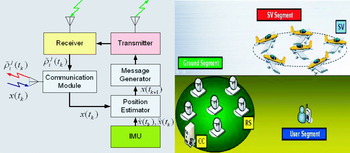
Figure 4. (Left) Block diagram representing a transceiver. (Right) Transceiver navigation system overview.

Navigation System Construction

Considering the properties of the mobile transceiver and its positioning algorithm, we propose a mobile transceiver-based navigation system as depicted in Figure 4 (Right). The system consists of a ground station, mobile satellite vehicle (SV), and user segment. The ground station segment consists of a computing centre (CC) and reference station (RS), placed at known positions. RSs receive navigation signals from the transceivers, and then transfer them to the CC. Transceivers also transmit their self-differenced observables to the CC. The CC estimates each SV's position by combining the gathered measurements, and then transmits the result to each SV. Several estimation methods for the SV position will be introduced in Section 4. After receiving the transmitted information, each SV compensates for a time delay and estimates its own position with the aid of an additional sensor such as an IMU. The transceiver then generates a stream of navigation messages based on the estimated position in real time and broadcasts it to the user segment. The transceiver can also generate a GPS-like signal, so the navigation user can get its own position using the on-the-shelf GNSS receiver. If the system operates independently of the existing GNSS, the navigation signal should have a different message and frequency. In this mode, the user receiver should be modified in order to receive its own signal.

Simulation Construction and Assumptions

To verify that this process can estimate the transceiver position more accurately than the existing algorithm and that the suggested system is feasible in a small country-sized region, the following simulation was performed. As shown in Figure 4 (Right), six RSs are considered in this simulation. One RS is located at the centre of a 100 km radius circle and the other five are on the circle perimeter. SVs are also distributed in the same manner as the RSs, but the optimal radius is varied with the transceiver coverage.

The transceiver coverage generally becomes larger as the SVs’ altitude increases, as shown in Table 2. Every coverage distance in Table 2 was calculated as a visible region on the earth sphere with an elevation cutoff angle of 5°. We aimed to implement a navigation system in a 700 km×900 km region, so the operating altitude should be higher than 40 km. To leave a margin, we chose 42 km as the SV altitude. Satellite vehicles with this capacity that are operating or being developed are the United Kingdom Zephyr and Helios of NASA.

Table 2. Transceiver coverage with increasing altitude (mask angle=5°).

Kovach (Reference Kovach2000) described a new user equivalent range error (UERE) budget for the modernized GPS. Based on this account, we reorganized the error budget of our suggested system in Table 3. The satellite vehicle remains in the stratosphere at an altitude of 42 km so the pseudorange of our system does not include any ionospheric delay error. As there is little gas or water vapour in the stratosphere, the UERE between the SVs is 0·46 m whereas that at the surface is 1·12 m.

Table 3. Error budget for the simulation.

Satellite Vehicle Positioning Methods

The RRP method can estimate the relative positions of all the transceivers as a self-calibrating pseudolite array as used by Stanford University (LeMaster et al., Reference LeMaster2002). To provide an absolute position to the user segment, a reference coordinate is necessary, and it is essential that the RSs are located at known positions as shown in Figure 5. We suggest that each RS and SV has a transceiver, but we also considered three additional algorithms in this simulation with which to compare the performance of the RRP method.

Figure 5. Concept of the transceiver positioning method.

We first estimated the position of the SV using the traditional IGPS. We considered only the receiver in the RS and the pseudolite in the SV in this method. We assumed that a reference clock could be located high enough to be visible from all the RSs. This clock eliminates the receiver clock bias (B _Rk) in each RS, and the CC estimates the pseudolite position and clock error as expressed in (8).

(8)

where: R _Rk: position vector of k-th RS.

We next considered a pseudolite-receiver set to be included in the SV segment. Each SV not only broadcasts the navigation signal, but also receives that of others as expressed in Equations (9) and (10).

(9)

(10)

The CC estimates the SV position, clock error of the pseudolite (b ⁱ), and clock bias of the receiver (B _j) using all the measurements from the RSs and SVs. This method is similar to the IGPS, so we call it the extended IGPS (EIGPS) in this paper.

The next step was to devise a real range positioning 1 (RRP 1) method that transceivers are only equipped with in an SV. The RSs still need the reference clock to eliminate their receiver clock bias. Using Equations (9) and (11), the CC can estimate the SVs' position and clock error. The real range (d _i^j) between the i-th and j-th SVs would help in estimating the positions.

(11)

The last method is RRP 2, where all the RSs and SVs have transceivers, and all the infrastructure segments can both receive and broadcast the signals. The reference clock is no longer necessary because the system does not need to eliminate the RS clock bias. The real range between SV and RS and between the pairs of SVs can determine the geometry and each SV can solve its absolute position by using Equation (12).

(12)

where: : a self-differenced measurement from the j-th transceiver to the k-th RS.

Case Study I – Normal Case

Let us consider a normal disposition of each segment. RSs that make a circle with the same distance would guarantee a good dilution of precision (DOP) value. SVs with an operating altitude of 42 km are located above the RS network as shown in Figure 6. The SVs would keep a flight formation designed to provide a consistent navigation performance. The optimal radius to cover a 350 km radius circular area at 42 km altitude is 160 km. We also considered the likelihood that the RSs are more spatially restricted than the mobile SVs, so the 100 km distance between the RSs is shorter than that for the SVs. The users are near the RSs and below the SVs. Each SV position should be estimated epoch-by-epoch because of the mobility, and users would get their own positions based on this error-included SV position each epoch. Table 4 summarizes the horizontal and vertical 2DRMS(distance root mean square) error of each method for each SV. The position accuracy of the central SV (#4) is precise regardless of the positioning method. All the methods can estimate this SV position to about 3 m accuracy. The outer SVs have greater position errors because of the geometry. The IGPS method is so sensitive that the 2DRMS errors are about 20 m. The RRP 2 method, which is used for the transceivers in SVs and RSs, guarantees a 5 m vertical accuracy (95%), being the best performance for all the mobile SVs.

Figure 6. Segment disposition in Case 1.

Table 4. Individual SV position accuracy for each method in Case 1.

Figure 7 shows the horizontal (left) and vertical (right) 2DRMS error distribution of all the users in the Case 1 service area. In these figures, the x axis is longitudinal and the y axis is latitudinal. The size of this service area is 700 km×600 km. The colour represents the 2DRMS error of each user. Users who are outside the SV network would have difficulty in determining their position accurately within an IGPS-based navigation environment. Alternatively, the EIGPS method can expand the available service area to a 300 km radius circular region within which users can estimate the horizontal position with 15 m accuracy and the vertical position with 25 m accuracy. The RRP 1 and 2 methods provide 10 m horizontal and 20 m vertical accuracy in a 350 km radius circular region.

Figure 7. Horizontal (left) and vertical (right) 2DRMS accuracy for surface users in Case 1. (In both diagrams: upper left – IGPS; upper right – EIGPS; lower left – RRP 1; lower right – RRP 2).

The average accuracies of all the user positions in a 700 km×600 km area are summarized in Table 5. The 50 m horizontal 2DRMS and 100 m vertical errors of the IGPS method are too great in practice. The average horizontal accuracy of other methods is about 15 m. The vertical error of EIGPS is about 30 m, whereas the performance of the RRP methods maintains the error at less than 20 m.

Table 5. Average accuracy of the user position for each SV positioning method in Case 1.

Case Study 2 – Distant RS Case

To provide a consistent navigational performance throughout the service area, all the segments should be located at their optimal disposition, as established in Case 1. However, we need to consider the extraordinary case in which a service area does not overlap with the reference station network. This system should work well to cover the area of a disaster such as a flood, fire, or building collapse. When users call for help in such a situation, as illustrated in Figure 8, there is little time to erect reference stations, but there is an immediate requirement for a navigation environment. We additionally considered users in the ocean or on a small island where RSs could not be located at a known fixed point. To test this extraordinary case we constructed a simulation array as in Figure 8. All the simulation conditions are the same as those in Case 1, except that the central SV of the constellation is 280 km horizontally distant from the central RS in the ground segment.

Figure 8. Segment disposition in Case 2.

In this case study, the IGPS method is unable to solve all the SV positions, because some lie beneath the 5° mask angle of the RS network. The horizontal results are less accurate than the Case 1 results by 1–3 m. The vertical errors become 5–7 times larger than the previous results. The furthest SV (#3) from the ground segment inevitably registers a vertical error of about 50 m with EIGPS, whereas RRP 1 and RRP 2 induce 35 m and 20 m errors, respectively. Figure 9 illustrates the user position accuracy in the service area of Case 2. As the abnormal disposition of the segments does not disrupt all the SVs’ horizontal positions, the user horizontal position accuracies are not greatly different from the results of Case 1. However, the vertical errors for some SVs are so large that these can become extreme near SV #3. In the worst case, a vertical 2DRMS error of 70 m can be experienced using the EIGPS method, whereas as much as 47 m (2DRMS) may be found using RRP 1. In contrast, the RRP 2 method can guarantee vertical accuracy within 25 m (2DRMS) in almost all the service area; this performance is largely acceptable.

Figure 9. Horizontal (left) and vertical (right) 2DRMS accuracy for a surface user in Case 2 (In both diagrams: upper left – EIGPS; upper right – RRP 1 – bottom: RRP 2).

Table 6 describes the 2DRMS error of each method for all the SVs in Case 2 and Table 7 shows the average accuracy for Case 2 in a 700 km×600 km area. The average horizontal accuracy of all the methods (EIGPS, RRP 1, and RRP 2) is about 15 m, a little less than that of Case 1. The vertical error of EIGPS is about 40 m, whereas the vertical performance of RRP 1 and RRP 2 would range around 30 m and 25 m, respectively.

Table 6. SV position accuracy for each method in Case 2.

Table 7. Average accuracy of user position for each SV positioning method in Case 2.

Case Study 3 – Network SV Case

In the Case 2 study, we found that vehicles far away from the RS network have poor vertical position accuracy. This is because the definite constraints imposed by the RS network are in the same general direction. Moreover, the signals from other directions from other SVs also contain errors. Additional constraints must be acquired from alternative directions and from an accurate point. Recalling that we can accurately estimate SV position near the RS network, a linkage between the constellations of Case 1 and Case 2, expressed in Figure 10, would be helpful. The accurately estimated SV positions would be relatively definite constraints, and the service area could be extended to a 700 km×900 km region. The horizontal and vertical accuracy of all the users in the 700 km×900 km service area of Case 3 is expressed in Figure 11. Most users for all the three methods can get their positions with a 10 m horizontal accuracy, but the vertical accuracy depends on the transceiver positioning technique. When the system uses the EIGPS method, 77% of the service area can achieve 25 m vertical accuracy, but some users will not achieve precision better than 50 m. The RRP 1 method can improve the user performance to within 45 m 2DRMS. The RRP 2 method not only removes the navigation shadow region, but also enlarges the area where all users can be satisfied with a 25 m vertical error.

Figure 10. Segment disposition in Case 3.

Figure 11. Horizontal (left) and vertical (right) 2DRMS accuracy for a surface user in Case 3 (In both diagrams: upper left – EIGPS; upper right – RRP 1; bottom – RRP 2).

Table 8 sets out the horizontal and vertical 2DRMS error results of each method for 10 SVs. The vertical position accuracy of the EIGPS is improved by 30–40%, and the horizontal accuracy of the RRP methods was enhanced by 10–20%. The RRP 2 method is still the most powerful estimation technique regardless of the SV constellation and the geometry of all the segments. Table 9 is the average accuracy result for the Case 3700 km×900 km area. The average horizontal 2DRMS accuracy of the EIGPS is about 16 m, and the vertical accuracy is 27 m, which is 30% better than Case 2. The results for RRP 1 are about 12 m horizontal and 23 m vertical accuracy. The most accurate technique, RRP 2, can provide 10 m horizontal and 19 m vertical accuracy.

Table 8. SV position accuracy for each method in Case 3.

Table 9. Average accuracy of user position for each SV positioning method in Case 3.

Consideration of SV Mobility

Finally, we considered the vehicle mobility effect. The optimal constellation array is disturbed when these platforms start moving. To maintain an optimized constellation, the flight formation illustrated in Figure 12 (Left) is necessary. The central SVs, #4 and #7, should hold to the central stationary point of each constellation and all the outer SVs need to move along a dumbbell-shaped trajectory with the same velocity and track.

Figure 12. Left – Formation flight of 10 SVs. Right – Views of horizontal accuracy variation with SV mobility.

Figure 12 (Right) shows the real-time horizontal position error variation in SV movement. We estimated each SV position using the RRP 2 method, and the disposition of all the navigation segments is the same as that of the Case 3 study. Users inside the SV network can consistently determine their position with an error of only 5 m, notwithstanding the SV mobility. Table 10 is the summary of position accuracy considering the SV mobility effect. The average 2DRMS error is about 12 m in the horizontal plane and about 21 m vertically. Degradations are only 1 m and 1·5 m, respectively. We can therefore construct an alternative navigation system whose 2DRMS performance with a variance of about 10 m horizontally and 20 m vertically in a 700 km×900 km region using mobile transceivers in formation flying vehicles.

Table 10. Average accuracy of user position for mobile SVs.