


1. Introduction
In this paper we give an arithmetic count of the lines on a smooth cubic surface in projective space  $\mathbf {P}_k^{3}$. A celebrated nineteenth-century result of Salmon and Cayley [Reference CayleyCay49] is that
 \begin{equation} \#\text{complex lines on}\ V = 27, \end{equation}
where  $V$ is such a surface over the complex numbers
  ${\mathbf {C}}$. In particular, this number is independent of the choice of
  $V$. By contrast, a real smooth cubic surface can contain
  $3$,
$3$,  $7$,
$7$,  $15$, or
  $27$ real lines.
It is a beautiful observation of Finashin and Kharlamov [Reference Finashin and KharlamovFK13] and of Okonek and Teleman [Reference Okonek and TelemanOT14a] that while the number of real lines on a smooth cubic surface depends on the surface, a certain signed count of lines is independent of the choice. Namely, the residual intersections of  $V$ with the hyperplanes containing
  $\ell$ are conic curves that determine an involution of
  $\ell$, defined so that two points are exchanged if they lie on a common conic. Lines are classified as either hyperbolic or elliptic according to whether the involution is hyperbolic or elliptic as an element of
  $\operatorname {PGL}_2$ (i.e. whether the fixed points are defined over
  $k$ or not). Finashin and Kharlamov [Reference Finashin and KharlamovFK13] and Okonek and Teleman [Reference Okonek and TelemanOT14a] observed that the equality
 \begin{equation} \#\text{real hyperbolic lines on}\ V - \#\text{real elliptic lines on}\ V = 3 \end{equation}
can be deduced from Segre's work. They gave new proofs of the result and extended it to more general results about linear subspaces of hypersurfaces. We review this and later work below.
We generalize these results to an arbitrary field  $k$ of characteristic not equal to 2. The result is particularly simple to state when
  $k$ is a finite field
  $\mathbb {F}_{q}$. As was observed in [Reference HirschfeldHir85, pp. 196–197], a line
  $\ell \subset V$ admits a distinguished involution, just as in the real case, and we classify
  $\ell$ as either hyperbolic or elliptic using the involution, as before.
When all  $27$ lines on
  $V$ are defined over
  $\mathbb {F}_{q}$, we prove that
 \[ \#\text{elliptic lines on}\ V = 0 \text{ mod 2.} \]
For  $V$ an arbitrary smooth cubic surface over
  $\mathbb {F}_{q}$, we have the following theorem.
Theorem 1 The lines on a smooth cubic surface  $V \subset \mathbf {P}^{3}_{\mathbb {F}_{q}}$ satisfy
 \begin{align} & \#\text{elliptic lines on}\ V\ \text{with field of definition}\ \mathbb{F}_{q^a}\ \text{for}\ a\ \text{odd} \nonumber\\ &\quad + \#\text{hyperbolic lines on}\ V\ \text{with field of definition}\ \mathbb{F}_{q^a}\ \text{for}\ a\ \text{even} = 0 \text{ (mod 2).} \end{align}
 Here a line means a closed point in the Grassmannian of lines in  $\mathbf {P}^3_k$, so a line corresponds to a Galois orbit of lines over an algebraic closure. For example, consider the Fermat surface
  $V = \{ x_1^3+x_2^3+x_3^3+x_4^3=0 \}$ over
  $\mathbb {F}_{q}$ of characteristic
  $p \ne 2, 3$. When
  $\mathbb {F}_{q}$ contains a primitive third root of unity
  $\zeta _{3}$, all the
  $27$ lines are defined over
  $\mathbb {F}_{q}$ and are hyperbolic. Otherwise
  $V$ contains three hyperbolic lines defined over
  $\mathbb {F}_{q}$ and
  $12$ hyperbolic lines defined over
  $\mathbb {F}_{q^2}$. (See § 2 for further discussion.)
For arbitrary  $k$, we replace the signed count valued in
  ${\mathbf {Z}}$ with a count valued in the Grothendieck–Witt group
  $\operatorname {GW}(k)$ of non-degenerate symmetric bilinear forms. (See [Reference LamLam05] or [Reference MorelMor12] for information on
  $\operatorname {GW}(k)$.) The signs are replaced by classes
  $\langle a \rangle$ in
  $\mathrm {GW}(k)$ represented by the bilinear pairing on
  $k$ defined by
  $(x, y) \mapsto a x y$ for
  $a$ in
  $k^*$. The class
  $\langle a \rangle$ is determined by arithmetic properties of the line, namely its field of definition and the associated involution, and we call this class the type of the line.
As we will discuss later, the reason for enumerating lines as elements of  $\operatorname {GW}(k)$ is that the Grothendieck–Witt group is the target of Morel's degree map in
  $\mathbf {A}^{1}$-homotopy theory. The types
  $\langle a \rangle$ are local contributions to an Euler number. Despite this underlying reason, the calculation of the types
  $\langle a \rangle$ as well as the proof of the arithmetic count are carried out in an elementary manner and without direct reference to
  $\mathbf {A}^{1}$-homotopy theory.
Theorem 1 is a special case of the following more general result. Let  $\ell$ be a line on
  $V$ and let
  $k \subseteq L$ denote the field of definition of
  $\ell$, which must be separable (Corollary 54). There is a transfer or trace map
  $\operatorname {Tr}_{L/k}: \mathrm {GW}(L) \to \mathrm {GW}(k)$ defined by taking a bilinear form
  $\beta : A \times A \to L$ on an
  $L$-vector space
  $A$ to the composition
  $\operatorname {Tr}_{L/k} \circ \beta : A \times A \to L \to k$ of
  $\beta$ with the field trace
  $\operatorname {Tr}_{L/k}: L \to k$, the vector space
  $A$ now being viewed as a vector space over
  $k$.
$k$.
We refine the classification of lines on  $V$ as either hyperbolic or elliptic as follows. Define the type of an elliptic line
  $\ell$ with field of definition
  $L$ to be the class
  $\mathcal {D} \in L^{\ast }/(L^{\ast })^2$ of the discriminant of the fixed locus, that is, to be the
  $\mathcal {D}$ such that
  $L(\sqrt {\mathcal {D}})$ is the field of definition of the fixed locus. We extend this definition by defining the type of a hyperbolic line to be
  $1$ in
  $L^{\ast }/(L^{\ast })^2$. Observe that when
  $k=\mathbb {R}$ (respectively,
  $\mathbb {F}_{q}$), the type of an elliptic line is
  $-1$ (respectively, the unique non-square class), but in general there are more possibilities. The type can also be interpreted in terms of the
  $\mathbf {A}^{1}$-degree of the involution. We explain this and other aspects of hyperbolic and elliptic lines in § 3.
With this definition of type, we now state the main theorem.
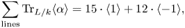
Theorem 2 (Main theorem) The lines on a smooth cubic surface  $V \subset \mathbf {P}^{3}_{k}$ satisfy
 \begin{equation} \sum_{h \in L^{{\ast}}/(L^{{\ast}})^{2}} \big( \#\text{lines of type}\ h\big) \cdot \operatorname{Tr}_{L/k}( \langle h \rangle) = 15 \cdot \langle 1 \rangle + 12 \cdot \langle -1 \rangle. \end{equation}
 From (4), we recover the complex count (1) by taking the rank of both sides, the real count (2) by taking the signature (the complex lines contribute the signature zero class  $\langle 1 \rangle + \langle -1 \rangle$), and the finite field count (3) by taking the discriminant (which is an element of
  $\mathbb {F}_{q}^{\ast }/(\mathbb {F}_{q}^{\ast })^{2} = \mathbb {Z}/2$).
Over a more general field, one gets analogues of those equations by taking the rank, discriminant, or signature (with respect to an ordering) of (4), but there can be more subtle constraints as well. For example, there is no smooth cubic surface over  $k=\mathbf {Q}$ with 27 lines defined over
  $k$, two with type
  $\langle 3 \rangle$, 13 with type
  $\langle 1 \rangle$, and 12 with type
  $\langle -1 \rangle$. Indeed, this is a special case of Theorem 2 because
  $2 \cdot \langle 3 \rangle + 13 \cdot \langle 1 \rangle + 11 \cdot \langle -1 \rangle$ and
  $15 \cdot \langle 1 \rangle + 12 \cdot \langle -1 \rangle$ have different Hasse–Witt invariants at the prime
  $p=3$. We cannot, however, rule out the existence of such a surface using the analogues of (1), (2), and (3) because the forms have the same rank, discriminant, and signature.
Theorem 2 only applies to a smooth cubic surface, but we discuss the singular surfaces at the end of this section, right before § 1.1.
The statement and proof of Theorem 2 are inspired by Finashin–Kharlamov and Okonek–Teleman's proof of the real line count (2), which in turn is inspired by a proof of the complex line count (1) that runs as follows. Let  $\mathcal {S}$ denote the tautological subbundle on the Grassmannian
  $G := \operatorname {Gr}(4, 2)$ of two-dimensional subspaces of the four-dimensional vector space
  $k^{\oplus 4}$. Given an equation
  $f \in \mathbb {C}[x_1, x_2, x_3, x_4]$ for a complex cubic surface
  $V\subset \mathbf {P}^{3}_{\mathbb {C}}$, the rule
 \[ \sigma_{f}(S) = f\,|\,S \]
determines a section  $\sigma _{f}$ of the vector bundle
  $\mathcal {E} = \operatorname {Sym}^{3}( \mathcal {S}^{\vee })$. By construction, the zeros of
  $\sigma _{f}$ are the lines contained in
  $S$, but a local computations shows that, when
  $S$ is smooth, the section
  $\sigma _{f}$ has only simple zeros, and so in this case the count of zeros equals the Chern number
  $c_{4}(\mathcal {E})$. We immediately deduce that the number of lines on a complex smooth cubic surface is independent of the surface, and it can be shown that this independent count is 27 by computing
  $c_{4}(\mathcal {E})$ using structural results about, for example, the cohomology of the complex Grassmannian.
The proofs by Finashin and Kharlamov and by Okonek and Teleman of the real count of lines are similar to the proof of the complex count just given. Both the real Grassmannian  $G(\mathbf {R})$ and the vector bundle
  $\mathcal {E}$ are orientable, so after fixing orientations, the Euler number
  $e(\mathcal {E})$ of
  $\mathcal {E}$ is well defined. The real count (2) can be proven along the same lines as the complex count, only with the Chern number replaced by the Euler number. One new complication is that, in addition to showing that
  $\sigma _{f}$ has only simple zeros, it is necessary to also show that the local index of a zero is
  $+1$ at a hyperbolic line and
  $-1$ at an elliptic line.
For this proof to generalize to a count over an arbitrary field, we need a generalization of the Euler number, which is furthermore computable as a sum of local indices. Classically, the local index of an isolated zero of a section  $\sigma$ can be computed by choosing local coordinates and a local trivialization, thereby expressing
  $\sigma$ as a function
  ${\mathbf {R}}^r \to {\mathbf {R}}^r$ with an isolated zero at the origin. The local degree of this function is then the local index, assuming that the choice of local coordinates and trivialization were compatible with a given orientation or relative orientation. In [Reference EisenbudEis78], Eisenbud suggested defining the local degree of a function
  $\mathbf {A}_k^r \to \mathbf {A}_k^r$ to be the isomorphism class of the bilinear form now appearing in the Eisenbud–Khimshiashvili–(Harold) Levine signature formula. This bilinear form is furthermore explicitly computable by elementary means. For example, if the Jacobian determinant
  $J$ is non-zero at a point with residue field
  $L$, then the local degree is
  $\operatorname {Tr}_{L/k} \langle J \rangle$. In [Reference Kass and WickelgrenKW19], we showed it is also the local degree in
  $\mathbf {A}^1$-homotopy theory.
Define the Euler number  $e(\mathcal {E}) \in \operatorname {GW}(k)$ to be the sum of the local indices using the described recipe and this local degree. Since local coordinates are not as well behaved for smooth schemes as for manifolds, some finite determinacy results are being used implicitly, but in the present case, these are elementary algebra. We show that the Euler number is well-defined using Scheja and Storch's perspective on duality for finite complete intersections (e.g. [Reference Scheja and StorchSS75]), which shows that this local degree behaves well in families.
The result is as follows. Let  $X$ be a smooth scheme of dimension
  $r$ over
  $k$. Let
  $\mathcal {E} \to X$ be a relatively oriented rank
  $r$ vector bundle such that any pair of sufficiently general sections can be connected by sections with only isolated zeros (as in Definition 37), potentially after further extensions of odd degree.
Theorem 3 The Euler number
 \[ e(\mathcal{E}) = \sum_{p \text{ such that } \sigma(p) = 0} \operatorname{ind}_p \sigma \]
is independent of the choice of section  $\sigma$.
This is shown as Corollary 38 in § 4, and some examples are computed. We deduce that the left-hand side of (4) is independent of the choice of surface. We then show that this common class equals the right-hand side of (4) by evaluating the count on a specially chosen smooth surface.
We remark that for  $f$ defining a smooth cubic surface, the corresponding section
  $\sigma _f$ has only simple zeros (the Jacobian determinant is non-zero), so the more general calculations of local degree from [Reference Scheja and StorchSS75, Reference Eisenbud and LevineEL77, Reference EisenbudEis78] are only needed here to ensure that the local degree behaves well in families [Reference Scheja and StorchSS75].
When  $f$ defines a singular cubic surface, the section
  $\sigma _{f}$ can have non-simple zeros. If we additionally assume
  $\sigma _{f}$ has only isolated zeros (i.e. the surface contains only finitely many lines), the index of a zero can be computing using the main result of [Reference Kass and WickelgrenKW19]. For example, when
  $f=x_0^2 x_3 + x_0 x_2^2+x_1^3$ (a surface with an
  $E_6$-singularity),
  $\sigma _{f}$ has a unique zero whose local index is described in [Reference Kass and WickelgrenKW19, § 7]. If the type of a line corresponding to a non-simple zero of
  $\sigma _{f}$ is defined to be the local index, then Theorem 2 remains valid for singular cubic surfaces containing only finitely many lines.
1.1 Relation to other work
A large number of Euler classes in arithmetic geometry have been constructed, but the definition used here seems to be original. Closest to our definition is that of Grigor‘ev and Ivanov in [Reference Grigor‘ev and IvanovGI80]. For a perfect field  $k$ of characteristic different from
  $2$, they consider the quotient
  $\Delta (k) = \mathrm {GW}(k)/\operatorname {TF}(k)$ of the Grothendieck–Witt group by the subgroup generated by trace forms of field extensions, and define the Euler number to be the element of
  $\Delta (k)$ given by the sum of the indices of the
  $k$-rational zeros of a chosen section with isolated zeros. Quotienting by the group generated by the trace forms allows them to ignore the zeros which are not
  $k$-rational. (See Proposition 34.) Their local index is also inspired by Eisenbud's article [Reference EisenbudEis78]. By contrast, they only consider orientations in the case of real closed field
  $k$, and the group
  $\Delta (k)$ is quite small, unless
  $k$ is algebraically closed or real closed: they show that for
  $k$ an algebraically closed field, the rank induces an isomorphism
  $\Delta (k) \cong \mathbb {Z}$; for
  $k$ a real closed field, the signature induces an isomorphism
  $\Delta (k) \cong \mathbb {Z}$; for fields where there is a fixed prime
  $p$ such that all extensions have degree
  $p^m$ and which are not algebraically closed or real closed, the rank determines an isomorphism
  $\Delta (k) \cong \mathbb {Z}/p$, and for all other fields
  $\Delta (k) = 0$. For example,
  $\Delta (k)$ is zero for a finite field or a number field, while the Grothendieck–Witt group of such fields is infinite and contains distinct elements with the same rank.
In  $\mathbf {A}^1$-homotopy theory, there is an Euler class in Chow–Witt groups, also called oriented Chow groups, twisted by the dual determinant of the vector bundle, defined by Barge and Morel [Reference Barge and MorelBM00] and by Fasel [Reference FaselFas08]: a rank
  $r$ vector bundle
  $E$ on a smooth
  $d$-dimensional scheme
  $X$ gives rise to an Euler class
  $e(E)$ in
  $\widetilde {\operatorname {CH}}^r(X, \det E^*)$. In [Reference MorelMor12, Chapter 8.2], Morel defines an Euler class in
  $H^r(X, \mathrm {K}^{\mathrm {MW}}_r (\det E^*))$ as the primary obstruction to the existence of a non-vanishing section. When the
  $\det E^*$ is trivial, Asok and Fasel used an isomorphism
  $H^r(X, \mathrm {K}^{\mathrm {MW}}_r (\det E^*)) \cong \widetilde {\operatorname {CH}}^r(X, \det E^*)$ (see [Reference Asok and FaselAF16, Theorem 2.3.4]), analogous to Bloch's formula for Chow groups, to show that these two Euler classes differ by a unit [Reference Asok and FaselAF16, Theorem 1] provided
  $k$ is a perfect field with
  $\operatorname {char} k \ne 2$. In a preprint that appeared while this paper was being written, Marc Levine extended this result to the case where the determinant is possibly non-trivial [Reference LevineLev17b, Proposition 11.6]. In the same paper, Levine also developed the properties of the Euler number or class of a relatively oriented vector bundle of rank
  $r$ on a smooth, proper
  $r$-dimensional
  $X$ defined by pushing forward the Euler class along the map
 \[ \widetilde{\operatorname{CH}}^r(X, \omega_{X/k}) \to \widetilde{\operatorname{CH}}^0(k) \cong \mathrm{GW}(k), \]
where  $\omega _{X/k}$ is the canonical sheaf and where the relative orientation is used to identify
  $\widetilde {\operatorname {CH}}^r(X, \det E^*)$ and
  $\widetilde {\operatorname {CH}}^r(X, \omega _{X/k})$. It is shown that this class coincides with
  $e(\mathcal {E})$ when our
  $e(\mathcal {E})$ is defined in [Reference Bachmann and WickelgrenBW02, Second Corollary, p. 3]. We give here a development of the Euler number in
  $\mathrm {GW}(k)$ which does not use the machinery of oriented Chow groups, and which is elementary in the sense that it only requires algebra to compute, along with some additional duality theory from commutative algebra to show it is well defined.
In earlier work, Nori, Bhatwadaker, Mandal, and Sridharan defined Euler class groups and weak Euler class groups for affine schemes. These have been used to study the question of when a projective module splits off a free summand [Reference Mandal and SridharanMS96, Reference Bhatwadekar and SridharanBS99, Reference Bhatwadekar and SridharanBS00, Reference Bhatwadekar, Das and MandalBDM06]. For smooth, affine varieties these groups can be mapped to the Chow–Witt groups in a way that is compatible with Euler classes under suitable additional hypotheses [Reference FaselFas08, Propositions 17.2.10, 17.2.11].
The signed count of real lines (2) on a cubic surface has been extended in various ways. Benedetti and Silhol gave a topological interpretation of the classification of lines as hyperbolic or elliptic using pin structures in [Reference Benedetti and SilholBS95]. The signed count can also be identified as an enumerative invariant defined in work of Solomon. In [Reference SolomonSol06], Solomon defined open Gromov–Witten invariants for a suitable real symplectic manifold of dimension 4 or 6. Solomon's invariants count certain real genus  $g$
$g$  $J$-holomorphic curves, and Finashin and Kharlamov explained in [Reference Finashin and KharlamovFK13, § 5.2] that (2) equals Solomon's invariant when
  $g=0$ and the symplectic manifold is the space of real points of the cubic surface. Solomon, together with Horev, also gave an alternative proof of (2) when the cubic surface is the blow-up of the plane in [Reference Horev and SolomonHS12], a paper in which they more generally compute the open Gromov–Witten invariants for certain blow-ups of the plane.
Another approach to studying the lines on a cubic surface is given by Basu, Lerario, Lundberg, and Peterson in [Reference Basu, Lerario, Lundberg and PetersonBLLP19]. They analyze the count of lines from the perspective of probability theory and give a new probabilistic proof of (2) [Reference Basu, Lerario, Lundberg and PetersonBLLP19, Proposition 2].
Finashin and Kharlamov [Reference Finashin and KharlamovFK13] and Okonek and Teleman [Reference Okonek and TelemanOT14a] compute more generally a signed count of the real lines on a hypersurface of degree  $2n-3$ in real projective space
  $\mathbf {P}^n_{\mathbb {R}}$. As in the case of cubic surfaces, this count is obtained as a computation of an Euler class, but unlike the case of cubic surfaces, care must be taken when defining the Euler class because the relevant real Grassmannian can be non-orientable, and the Euler number is often only defined for oriented vector bundles on an oriented manifold. The two sets of researchers address this complication in different ways. Finashin and Kharlamov work on the orientation cover of
  $G(\mathbf {R})$ and orient the pullback of
  $\mathcal {E}$. By contrast, Okonek and Teleman work on
  $G(\mathbf {R})$ and construct a suitably defined relative orientation of
  $\mathcal {E}$ with an associated Euler class. These results are also analyzed by Basu, Lerario, Lundberg, and Peterson using tools from probability in [Reference Basu, Lerario, Lundberg and PetersonBLLP19]. Further extensions of these ideas are found in [Reference Finashin and KharlamovFK15, Reference Okonek and TelemanOT14b].
The work described in the present paper is part of a broader program aimed at using  $\mathbf {A}^1$-homotopy theory to prove arithmetic enrichments of results in enumerative geometry, with earlier results by Marc Hoyois [Reference HoyoisHoy14], the present authors [Reference Kass and WickelgrenKW19], and Marc Levine [Reference LevineLev17a, Reference LevineLev17b]. After a version of this paper was posted to the arXiv, additional results were obtained by Marc Levine [Reference LevineLev18, Reference LevineLev19], Stephen McKean [Reference McKeanMcK21], Sabrina Pauli [Reference PauliPau20], Padma Srinivasan with the second author [Reference Srinivasan and WickelgrenSW18], and Matthias Wendt [Reference WendtWen20]. The most closely related of these results are Levine's [Reference LevineLev19] and Pauli's [Reference PauliPau20]. Levine computes the
  ${\mathbf {A}}^1$-Euler number of
  $\operatorname {Sym}^{2n-5} {\mathcal {S}}^*$ on
  $\operatorname {Gr}(n,2)$, and Pauli analyzes the lines on the quintic
  $3$-fold.
2. Notation and conventions
Given a  $k$-vector space
  $A$ and an integer
  $r$, the Grassmannian parameterizing
  $r$-dimensional subspaces of
  $A$ will be denoted by
  $\operatorname {Gr}(A, r)$. We will write
  $\operatorname {Gr}(n, r)$ for
  $\operatorname {Gr}( k^{\oplus n}, r)$.
  $\mathbf {P}(A)$ is
  $\operatorname {Gr}(A, 1)$ or equivalently
  $\operatorname {Proj}( \operatorname {Sym}(A^{\vee }))$. With this convention,
  $H^{0}( \mathbf {P}(A), {\mathcal {O}}(1)) = A^{\vee }$.
  $\mathbf {P}^{n}_{k}$ is
  $\mathbf {P}(k^{\oplus n+1})$. The standard basis of
  $k^{\oplus 4}$ is
  $(1, 0, 0, 0), (0, 1, 0, 0), (0, 0, 1, 0), (0, 0, 0, 1)$. The dual basis of
  $(k^{\oplus 4})^{\vee }$ is denoted
  $x_1, x_2, x_3, x_4$.
A linear system on a projective  $k$-variety
  $V$ is a pair
  $(T, {\mathcal {L}})$ consisting of a line bundle
  ${\mathcal {L}}$ and a subspace
  $T \subset H^{0}(V, {\mathcal {L}})$ of the space of global sections. The linear system
  $(T, {\mathcal {L}})$ is base-point-free if
  $\cap _{s \in T} \{ s=0 \}$ is the empty subscheme. If
  $(T, {\mathcal {L}})$ is base-point-free, then there is a unique morphism
  $\pi \colon V \to \mathbf {P}(T^{\vee })$ together with an isomorphism
  $\pi ^{*}{\mathcal {O}}(1) \cong {\mathcal {L}}$ that induces the identity on
  $T$.
$T$.
In general, calligraphic font denotes a family of objects, such as  $\mathcal {E}$ denoting a vector bundle because it is a family of vector spaces. However, when there is a family of vector bundles, the family then is denoted
  $\mathcal {E}$.
The concept of a line on a scheme over the possibly non-algebraically closed field  $k$ is slightly subtle and plays a fundamental role here. We use the following definition.
Definition 4 A line  $\ell$ in
  $\mathbf {P}^{3}_{k}$ is a closed point of
  $\operatorname {Gr}(4, 2)$. The residue field of this closed point is called the field of definition of
  $\ell$.
To a line  $\ell$ with field of definition
  $L$, there is the following associated closed subscheme of
  $\mathbf {P}^{3}_{L}$. The closed point
  $\ell \in \operatorname {Gr}(4, 2)$ defines a morphism
  $\operatorname {Spec}(L) \to \operatorname {Gr}(4, 2)$. If the pullback of the tautological subbundle under this morphism is the rank
  $2$ submodule
  $S \subset L^{\oplus 4}$, then the homogeneous ideal generated by
  $\operatorname {ann}(S) \subset \operatorname {Sym} ((L^{4})^{\vee })$ defines a subscheme of
  $\mathbf {P}^{3}_{L}$. By abuse of notation we denote this subscheme by
  $\ell$.
For  $a$ in
  $k^*$, the element of the Grothendieck–Witt group
  $\mathrm {GW}(k)$ represented by the symmetric, non-degenerate, rank
  $1$ bilinear form
  $(x,y) \mapsto a xy$ for all
  $x,y$ in
  $k$ is denoted by
  $\langle a \rangle$.
3. Hyperbolic and elliptic lines
Here we define the type of a line on a cubic surface over an arbitrary field  $k$ of characteristic different than
  $2$, define hyperbolic and elliptic lines, and derive an explicit expression for the type (Proposition 14). This expression will be used in § 5 to relate the type to a local
  $\mathbf {A}^{1}$-Euler number.
We fix a cubic polynomial  $f \in k[x_1, x_2, x_3, x_4]$ that defines a
  $k$-smooth cubic surface, which we denote by
  $V := \{ f=0 \} \subset \mathbf {P}^{3}_{k}$.
Definition 5 Suppose that  $\ell$ is a line contained in
  $V$, with field of definition
  $L$. Define
  $T\subset (L^{\oplus 4})^{\vee } = H^{0}( \mathbf {P}_{L}^{3}, {\mathcal {O}}(1))$ to be the vector space of linear polynomials that vanish on
  $\ell$. This vector space is naturally a subspace of the space of global sections of
  ${\mathcal {O}}_{V}(1)$ and the space of global sections of the sheaf
  $I_{\ell }(1) := I_{\ell } \otimes {\mathcal {O}}_{V}(1)$ of linear polynomials vanishing on
  $\ell$.
The subspace  $T$ can alternatively be described as
  $T = \operatorname {ann}(S)$ for
  $S \subset L^{\oplus 4}$ the subspace corresponding to
  $\ell$.
The ideal sheaf  $I_{\ell }$ is a line bundle because
  $\ell$ is a codimension
  $1$ subscheme of the smooth surface
  $V \otimes _{k} L$. Thus
  $T$ defines two linear systems on
  $V \otimes _{k} L$: the linear system
  $(T, {\mathcal {O}}_V(1))$ and the linear system
  $(T, I_{\ell }(1))$. The elements
  $(T, {\mathcal {O}}_V(1))$ are the intersections with planes containing
  $\ell$, while the elements of
  $(T, I_{\ell }(1))$ are the residual intersections with these planes. The linear system
  $(T, {\mathcal {O}}_V(1))$ has base-points, namely the points of
  $\ell$, but as the following lemma shows, the other linear system is base-point-free.
Lemma 6 The linear system  $(T, I_{\ell }(1))$ is base-point-free.
Proof. The sheaf  $I_{\ell }(1)$ is the restriction of the analogous sheaf on
  $\mathbf {P}^{3}_{L}$, and the sheaf on
  $\mathbf {P}^{3}_{L}$ is generated by
  $T$ by the definition of the subscheme
  $\ell \subset \mathbf {P}^{3}_{L}$ (see § 2). We conclude that the same holds on
  $V$, and
  $T$ generating
  $I_{\ell }(1)$ is equivalent to base-point-freeness.
Definition 7 Let  $\pi \colon V \otimes L \to \mathbf {P}(T^{\vee })$ be the morphism associated to the base-point-free linear system
  $(T, I_{\ell }(1))$. The restriction of
  $\pi$ to
  $\ell$ is a finite morphism of degree
  $2$ (see Lemma 10), hence is Galois (as
  $\operatorname {char} k \ne 2$). We denote the non-trivial element of the Galois group of
  $\ell \to \mathbf {P}(T^{\vee })$ by
 \[ i \colon \ell \to \ell. \]
 The involution  $i$ is the one discussed in the introduction. Concretely,
  $\pi$ is the unique morphism that extends projection from
  $\ell$. One may identify
  $\mathbf {P}(T^{\vee })$ with the space of planes in
  $\mathbf {P}^{3}_{L}$ containing
  $\ell$. Under this identification,
  $\pi$ sends a point
  $p$ to the tangent space
  $T_pV$ to
  $V$ at
  $p$ viewed as a projective plane of dimension
  $2$, and therefore the involution
  $i$ swaps
  $p$ and
  $q$ if and only if
  $T_p V = T_q V$. Note that the intersection of
  $T_pV$ with
  $V$ is a degree
  $3$ plane curve containing
  $\ell$, which can therefore be described as a conic
  $Q$ union
  $\ell$. We see that
  $\pi$ should be degree
  $2$ because, given a point
  $p$ of
  $\ell$, the intersection of
  $Q$ with
  $\ell$ contains two points (counted with multiplicity), and these are precisely the points with the same tangent space.
Remark 8 Recall that we require  $\operatorname {char} k \ne 2$, and this requirement is important because otherwise the involution
  $i$ might not exist, in which case the type is undefined. Indeed, consider the surface
  $V$ over
  $\mathbb {F}_{2}$ defined by
  $f = x_{1}^3+x_{2}^3+x_{3}^3+x_{4}^3$. This surface contains the line
  $\ell$ defined by the subspace spanned by
  $(1, 1, 0, 0)$ and
  $(0, 0, 1, 1)$. The morphism
  $\pi \colon \ell \to \mathbf {P}(T^{\vee })$ is purely inseparable, as can be seen by either direct computation or an application of Lemma 10 below. In particular,
  $\ell$ does not admit a non-trivial automorphism that respects
  $\pi$.
Having defined  $i$, we can now define hyperbolic and elliptic lines in direct analogy with Segre's definition. We use Morel's
  $\mathbf {A}^{1}$-Brouwer degree, as constructed in [Reference MorelMor12].
Definition 9 The type of a line on  $V$ is
  $\langle -1 \rangle \cdot \deg ^{\mathbf {A}^{1}}(i)$, the product of
  $\langle -1 \rangle$ and the
  $\mathbf {A}^{1}$-degree of the associated involution
  $i$. We say that the line is hyperbolic if the type equals
  $\langle 1 \rangle$ (i.e.
  $\deg ^{\mathbf {A}^{1}}(i) = \langle -1 \rangle$). Otherwise we say that the line is elliptic.
The general definition of the  $\mathbf {A}^{1}$-degree is complicated, but
  $\deg ^{\mathbf {A}^{1}}(i)$ has a simple description. If we identify
  $\ell$ with
  $\mathbf {P}_{L}^{1}$ so that
  $i$ is the linear fractional transformation
  $(\alpha z+\beta )/(\gamma z +\delta )$, then the
  $\mathbf {A}^{1}$-degree is
  $\langle \alpha \delta - \beta \gamma \rangle \in \operatorname {GW}(k)$. In particular,
  $\ell$ is hyperbolic if and only if
  $-(\alpha \delta - \beta \gamma )$ is a perfect square in
  $L$.
$L$.
We define the type to be the negative of the degree rather than the degree itself so that, when  $k=\mathbb {R}$, the type is consistent with the sign conventions in [Reference Finashin and KharlamovFK13, Reference Okonek and TelemanOT14a]. There hyperbolic lines are counted with sign
  $+1$ and elliptic lines with sign
  $-1$.
$-1$.
We now derive an expression for the fibers of  $\pi \colon \ell \to \mathbf {P}(T^{\vee })$.
Lemma 10 Suppose that  $V$ contains the line
  $\ell$ defined by the subspace spanned by
  $(0,0,1,0)$ and
  $(0, 0, 0, 1)$. Write
 \[ f = x_{1} \cdot P_1 + x_{2} \cdot P_2 \]
for homogeneous quadratic polynomials  $P_1, P_2 \in k[x_1, x_2, x_3, x_4]$.
Then the fiber of  $\pi \colon \ell \to \mathbf {P}(T^{\vee })$ over the
  $k$-point corresponding to the one-dimensional subspace spanned by
  $(a, b, 0, 0) \in T^{\vee }$ is
 \begin{equation} \{ a \cdot P_{1}(0, 0, x_{3}, x_{4}) + b \cdot P_{2}(0, 0, x_{3}, x_{4})=0 \} \subset \ell . \end{equation}
Proof. The point corresponding to  $(a, b, 0, 0)$ is the zero locus of
  $b x_{1} - a x_{2}$, considered as a global section of
  ${\mathcal {O}}_{\mathbf {P}(T^{\vee })}(1)$. By construction, the preimage of this point under
  $\pi \colon \ell \to \mathbf {P}( T^{\vee })$ is the zero locus of
  $b x_{1} - a x_{2}$ considered as a global section of
  ${\mathcal {O}}_{\ell } \otimes I_{\ell }(1)$. We prove the lemma by identifying
  ${\mathcal {O}}_{\ell } \otimes I_{\ell }(1)$ with
  ${\mathcal {O}}_{\ell }(2)$ in such a way that
  $b x_{1} - a x_{2}$ is identified with the polynomial in (5).
Consider the line bundle  $I_{\ell }(1)$. On
  $V$, we have
  $0 = x_{1} P_1 + x_{2} P_2$, so
  $x_{1} = - P_{2}/P_{1} \cdot x_{2}$, showing that
  $x_{2}$ generates
  $I_{\ell }(1)$ on
  $\{ P_1 \ne 0 \}$ and
  $x_{1}$ generates
  $I_{\ell }(1)$ on
  $\{ P_{2} \ne 0 \}$. We conclude that the analogue is true for
  ${\mathcal {O}}_{\ell } \otimes I_{\ell }(1)$, and the map sending
  $x_{2}$ to
  $-P_{1}(0, 0, x_{3}, x_{4})$ and
  $x_{1}$ to
  $P_{2}(0, 0, x_{3}, x_{4})$ defines an isomorphism
  ${\mathcal {O}}_{\ell } \otimes I_{\ell }(1) \cong {\mathcal {O}}_{\ell }(2)$ that sends
  $b x_{1} - a x_{2}$ to
  $a P_{1}(0, 0, x_{3}, x_{4}) + b P_{2}(0, 0, x_{3}, x_{4})$.
We now collect some general results about involutions and then apply those results to get a convenient expression for  $\deg ^{\mathbf {A}^{1}}(i)$.
Lemma 11 Every non-trivial involution  $i \colon \mathbf {P}^{1}_{k} \to \mathbf {P}^{1}_{k}$ is conjugate to the involution
  $z \mapsto -\alpha /z$ for some
  $\alpha \in k$.
Proof. This is [Reference BeauvilleBea10, Theorem 4.2].
Lemma 12 The  $\mathbf {A}^1$-degree of
  $i(z) = -\alpha /z$ is
  $\langle \alpha \rangle \in \operatorname {GW}(k)$.
Proof. This is a special case of, for example, the main result of [Reference CazanaveCaz12].
Corollary 13 If  $i$ is a non-trivial involution on
  $\mathbf {P}^{1}_{k}$ and
  $\mathcal {D} \in k$ is the discriminant of the fixed subscheme of
  $i$, then
 \[ \langle -1 \rangle \cdot \deg^{\mathbf{A}^{1}}(i) = \langle \mathcal{D} \rangle \quad\text{in}\ \operatorname{GW}(k). \]
Proof. Both the  $\mathbf {A}^{1}$-degree and the class of the discriminant are unchanged by conjugation, so by Lemma 11, it is enough to prove the result when
  $i$ is the involution
  $i(z) = -\alpha /z$. In this case, the fixed subscheme is
  $\{ z^2+\alpha =0 \}$, which has discriminant
  $-4 \alpha$. We have that
  $\langle -4 \alpha \rangle = \langle -\alpha \rangle$, and the second class is
  $\langle -1 \rangle \cdot \deg ^{\mathbf {A}^{1}}(i)$ by Lemma 12.
Proposition 14 Let  $e_1, e_2, e_3, e_4$ be a basis for
  $k^{\oplus 4}$ such that the subspace
  $S := k \cdot e_3 + k \cdot e_4$ defines a line contained in
  $V$. Let
  $x_1, x_2, x_3, x_4$ denote the dual basis to
  $e_1, e_2, e_3, e_4$. Then the associated involution satisfies
 \begin{equation} \langle -1 \rangle \cdot \deg^{\mathbf{A}^{1}}(i) = \left\langle \operatorname{Res}\left(\left.\frac{\partial f}{\partial x_1}\right|S, \left.\frac{\partial f}{\partial x_2}\right|S \right) \right\rangle\quad \text{in}\ \operatorname{GW}(k). \end{equation}
Remark 15 Note that the resultant in (6) should be understood as the resultant of homogeneous polynomials in  $x_3$ and
  $x_4$. The choices of bases are not significant because different choices would change the resultant by a perfect square, leaving the class in
  $\operatorname {GW}(k)$ unchanged.
Remark 16 For any line  $\ell$, we may choose a basis such that
  $\ell$ corresponds to a subspace
  $S := L \cdot e_3 + L \cdot e_4$, where
  $L=k(\ell )$ is the field of definition of
  $\ell$. Proposition 14 then implies the equality
  $\langle -1 \rangle \cdot \deg ^{\mathbf {A}^{1}}(i) = \langle \operatorname {Res}( ({\partial f}/{\partial x_1})\,|\,S, ({\partial f}/{\partial x_2})\,|\,S ) \rangle$ in
  $\operatorname {GW}(L)$.
Proof. By Corollary 13, it is enough to show that the right-hand side of (6) equals the class of the discriminant of the fixed locus of  $i$. This fixed locus maps isomorphically onto the ramification locus of
  $\pi \colon \ell \to \mathbf {P}( T^{\vee })$, and we compute by directly computing the discriminant of the ramification locus using Lemma 10 as follows.
If we write  $f = x_{1} P_{1} + x_{2} P_{2}$, then Lemma 10 implies that the ramification locus is the locus where the polynomial
 \begin{equation} a \cdot P_1(0, 0, x_{3}, x_{4})+ b \cdot P_2(0, 0, x_{3}, x_{4}) \end{equation}
in  $x_{3}, x_{4}$ has a multiple root. The ramification locus is thus the zero locus of
  $\operatorname {Disc}_{x_{3}, x_{4}}( a \cdot P_{1}(0, 0, x_{3}, x_{4}) + b \cdot P_{2}(0, 0, x_{3}, x_{4}))$, the discriminant of (7) considered as a polynomial in
  $x_{3}$ and
  $x_{4}$. Consequently the discriminant of the ramification locus is
  $\operatorname {Disc}_{a, b}( \operatorname {Disc}_{x_{3}, x_{4}}( a \cdot P_{1}(0, 0, x_{3}, x_{4}) + b \cdot P_{2}(0, 0, x_{3}, x_{4}))) \in k^{\ast }/ (k^{\ast })^{2}$.
The right-hand side of (6) can also be described in terms of  $P_{1}, P_{2}$. Differentiating
  $f = x_{3} P_{1} + x_{4} P_{2}$, we get
  $({\partial f}/{\partial e_1})\,|\,S = P_{1}(0, 0, x_{3}, x_{4})$ and
  $({\partial f}/{\partial e_2}) = P_{2}(0, 0, x_{3}, x_{4})$. We now complete the proof by computing explicitly. If
  $P_1(0, 0, x_{3}, x_{4}) = \sum a_{i} x_{3}^{i} x_{4}^{2-i} \text { and } P_{2}(0, 0, x_{3}, x_{4}) = \sum b_{i} x_{3}^{i} x_{4}^{2-i}$, then resultant computations show
 \begin{align*} & \operatorname{Res}(P_1(0, 0, x_{3}, x_{4}), P_2(0, 0, x_{3}, x_{4}))\\ &\quad = a_1^2 b_0 b_2-a_2 a_1 b_0 b_1-a_0 a_1 b_1 b_2 +a_2^2 b_0^2+a_0 a_2 b_1^2 + a_0^2 b_2^2-2 a_0 a_2 b_0 b_2 \\ &\quad = \frac{1}{16} \operatorname{Disc}_{a,b}(\operatorname{Disc}_{x_{3},x_{4}} (a \cdot P_{1}(0, 0, x_{3}, x_{4})+ b \cdot P_{2}(0, 0, x_{3}, x_{4}))). \end{align*}
4. Euler number for relatively oriented vector bundles
In this section we define an Euler number in  $\mathrm {GW}(k)$ for an algebraic vector bundle which is appropriately oriented and has a sufficiently connected space of global sections with isolated zeros. The definition is elementary in the sense that it can be calculated with linear algebra. Some duality theory from commutative algebra as in [Reference BeauvilleBea71, Reference Eisenbud and LevineEL77, Reference Scheja and StorchSS75] is used to show that the resulting element of
  $\mathrm {GW}(k)$ is well defined, but no tools from
  $\mathbf {A}^1$-homotopy theory are needed. The precise hypothesis we use on sections is given in Definition 38. The precise hypothesis on orientations is that the vector bundle be relatively oriented as in Definition 17. The vector bundle is assumed to be on a smooth
  $k$-scheme with
  $k$ a field.
An alternative approach using Chow–Witt groups or oriented Chow groups of Barge and Morel [Reference Barge and MorelBM00] and Fasel [Reference FaselFas08] is developed in the work of Marc Levine [Reference LevineLev17b] without the hypothesis on sections. See the introduction for further discussion.
Let  $\pi : E \to X$ be a rank
  $r$ vector bundle on a smooth dimension
  $r$ scheme
  $X$ over
  $k$. In [Reference MorelMor12, Definition 4.3], an orientation of
  $E$ is a line bundle
  $L$ and an isomorphism
  $L^{\otimes 2} \cong \wedge ^{\mathrm {top}} E.$ Following Okonek and Teleman [Reference Okonek and TelemanOT14a], we make use of the related concept of a relative orientation.
Let  ${\mathcal {T}}(X) \to X$ denotes the tangent bundle.
Definition 17 A relative orientation of  $E$ is a pair
  $(L, j)$ consisting of a line bundle
  $L$ and an isomorphism
  $j: L^{\otimes 2} \stackrel {\cong }{\to } \operatorname {Hom}(\wedge ^{\mathrm {top}}{\mathcal {T}}(X), \wedge ^{\mathrm {top}}E)$.
Assume furthermore that  $\pi : E \to X$ is relatively oriented. On an open
  $U$ of
  $X$, we say that a section
  $s$ of
  $\operatorname {Hom}(\wedge ^{\mathrm {top}}{\mathcal {T}}(X), \wedge ^{\mathrm {top}}E)$ is a square if its image under
 \[ \Gamma (U, \operatorname{Hom}({\wedge}^{\mathrm{top}}{\mathcal{T}}(X), \wedge^{\mathrm{top}}E) ) \cong \Gamma (U, L^{{\otimes} 2} ) \]
is the tensor square of an element in  $\Gamma (U, L)$.
Let  $p$ be a closed point of
  $X$, which as above is a smooth dimension
  $r$ scheme over
  $k$.
$k$.
Definition 18 An étale map
 \[ \phi: U \to \mathbf{A}_k^r = \operatorname{Spec} k[x_1, \ldots, x_r] \]
from an open neighborhood  $U$ of
  $p$ to the affine space, which induces an isomorphism on the residue field of
  $p$, is called Nisnevich coordinates around
  $p$.
$p$.
Lemma 19 There are Nisnevich coordinates around any closed point whose residue field is separable over  $k$ for
  $r \geq 1$.
(When  $r=0$, this result does not hold. For a counter-example, consider
  $\operatorname {Spec} L \to \operatorname {Spec} k$ for a non-trivial, finite, separable extension
  $k \subseteq L$.)
Proof. Let  $X \to \operatorname {Spec} k$ be smooth of dimension
  $r \geq 1$ and let
  $p$ be a closed point of
  $X$ such that
  $k \subseteq k(p)$ is separable. We may assume that
  $X$ is affine. Let
  $p$ also denote the ideal corresponding to
  $p$. By [SGA1, II Corollaire 5.10 and 5.9], there are
  $x_1, \ldots , x_r$ in
  $\mathcal {O}_X$ such that
  $x_1, \ldots , x_r$ generate
  $p$. Since
  $k \subseteq k(p)$ is separable, there is
  $x \in \mathcal {O}_X$ which generates
  $k(p)$ as an extension of
  $k$ by the primitive element theorem. If
  ${\textrm {d}x}$ is zero in
  $\Omega _{X/k}^1 \otimes k(p)$, then
  $d (x + x_1), d x_2 ,\ldots , d x_r$ is a
  $k(p)$-basis of
  $\Omega _{X/k}^1 \otimes k(p)$, whence
  $X \to \operatorname {Spec} k [x + x_1, x_2, \ldots , x_r]$ is étale at
  $p$. Furthermore,
  $x + x_1 = x$ modulo
  $p$. It follows that the map
  $X \to \operatorname {Spec} k [x + x_1, x_2, \ldots , x_r]$ gives Nisnevich coordinates around
  $p$. If
  ${\textrm {d}x}$ is non-zero in
  $\Omega _{X/k}^1 \otimes k(p)$, then we may use
  ${\textrm {d}x}$ as the first basis element in a basis formed from the spanning set
  $\{ {\textrm {d}x}, dx_1, \ldots , dx_r \}$. The map to
  $r$-dimensional affine space over
  $k$ corresponding to this basis gives Nisnevich coordinates.
Proposition 21 There are Nisnevich coordinates around any closed point of a smooth  $k$-scheme of dimension
  $r\geq 1$.
Proof. Nisnevich coordinates exist around closed points of smooth  $r$-dimensional
  $k$-schemes when
  $k$ is infinite and
  $r\geq 1$ by [Reference KnusKnu91, Chapter 8, Proposition 3.2.1]. Combining with the previous lemma, we have the claimed existence of Nisnevich coordinates.
We thank Alexey Ananyevskiy and Ivan Panin for the reference to [Reference KnusKnu91].
Let  $\phi$ be Nisnevich coordinates around
  $p$. Since
  $\phi$ is étale, the standard basis for the tangent space of
  $\mathbf {A}_k^r$ gives a trivialization for
  $TX \vert _U$. By potentially shrinking
  $U$, we may assume that the restriction of
  $E$ to
  $U$ is trivial.
Definition 22 A trivialization of  $E\vert _U$ will be called compatible with Nisnevich coordinates
  $\phi$ and the relative orientation if the element of
  $\operatorname {Hom}(\wedge ^{\mathrm {top}}{\mathcal {T}}(X)\vert _U, \wedge ^{\mathrm {top}}E\vert _U)$ taking the distinguished basis of
  $\wedge ^{\mathrm {top}}{\mathcal {T}}(X)\vert _U$ to the distinguished basis of
  $\wedge ^{\mathrm {top}}E\vert _U$ is a square.
Given  $\phi$ and a compatible trivialization of
  $E\vert _U$, let
  $r_U$ in
  $\Gamma (U, L)$ denote an element such that
  $r_U^{\otimes 2}$ maps to the distinguished section of
  $\operatorname {Hom}(\wedge ^{\mathrm {top}}{\mathcal {T}}(X)\vert _U, \wedge ^{\mathrm {top}}E\vert _U)$ under the relative orientation.
Let  $\sigma$ in
  $\Gamma (X, E)$ denote a section, and let
  $Z \subseteq X$ denote the closed subscheme
  $\{ \sigma =0\}$.
Definition 23 A point  $p$ of
  $Z$ is said to be an isolated zero of
  $\sigma$ if the local ring
  $\mathcal {O}_{Z,p}$ is a finite
  $k$-algebra. We say that the section
  $\sigma$ has isolated zeros if
  $\mathcal {O}_Z$ is a finite
  $k$-algebra.
A section  $\sigma$ has isolated zeros if every zero is isolated and
  $X$ is connected.
Proposition 24 The following are equivalent characterizations of an isolated zero of a section  $\sigma$, and of
  $\sigma$ having isolated zeros.
•
 $p$ is an isolated zero of $\sigma$ if and only if there is a Zariski open neighborhood $U$ of $p$ such that the set-theoretic intersection $U \cap Z$ is $p$, that is, $U \cap Z= \{ p\}$.
•
$\sigma$ has isolated zeros if and only if $Z$ consists of finitely many closed points.


Proof. If  $p$ is an isolated zero of
  $\sigma$, then
  $\mathcal {O}_{Z,p}$ is dimension zero. Since
  $p$ is a closed point,
  $\mathcal {O}_{Z,p}/p$ has dimension zero. Let
  $Z^0$ be an irreducible component of
  $Z$ containing
  $p$. Since
  $Z^0$ is finite type over a field,
  $\dim Z^0 = \dim \mathcal {O}_{Z,p} + \dim \mathcal {O}_{Z,p}/p = 0$. Thus
  $Z^0$ is an irreducible dimension zero scheme which is finite type over
  $k$ and is therefore a single point, which must be
  $p$. Thus we may take
  $U$ to be the complement of the other irreducible components of
  $Z$.
$Z$.
If  $p$ is a closed point with a Zariski open neighborhood
  $U$ such that
  $U \cap Z= \{ p\}$, then
  $\dim Z^0 =0$. A zero-dimensional finite type
  $k$-algebra is finite.
Since a zero-dimensional Noetherian ring has finitely many points, if  $\sigma$ has isolated zeros, then
  $Z$ has finitely many points. These points are closed because since
  $Z$ is closed, any specialization of a point of
  $Z$ is in
  $Z$, and since
  $Z$ is zero-dimensional, there are no such specializations.
If  $Z$ consists of finitely many closed points, then
  $Z$ is a zero-dimensional finite type
  $k$-algebra, which is thus finite.
We will use Nisnevich coordinates around  $p$ and a local trivialization of
  $E$ to express the section
  $\sigma$ of
  $E$ as a function
  $\mathbf {A}^r_k \to \mathbf {A}^r_k$ plus an error term in a high power of the ideal corresponding to
  $p$. This will allow us to use a notion of local degree of a function
  $\mathbf {A}^r_k \to \mathbf {A}^r_k$ to define the local contribution to the Euler number. To do this, we will relate local rings
  $\mathcal {O}_{X,p}$ and
  $\mathcal {O}_{Z,p}$ of
  $p$ to the coordinate functions coming from the Nisnevich coordinates. The ideal corresponding to
  $p$ will also be denoted by
  $p$.
$p$.
Lemma 25 Let  $p$ be an isolated zero of the section
  $\sigma$, and let
  $\phi : U \to \mathbf {A}_k^r = \operatorname {Spec} k[x_1, \ldots , x_r]$ be Nisnevich coordinates around
  $p$. Then we have the following assertions.
•
$\mathcal {O}_{Z,p}$ is generated as a $k$-algebra by $x_1,\ldots ,x_r$. (We identify the $x_i$ with their pullbacks $\phi ^* x_i$.)• For any positive integer
$m$, the local ring $\mathcal {O}_{X,p}/p^{m}$ is generated as a $k$-algebra by $x_1,\ldots ,x_r$.


Proof. Since  $\mathcal {O}_{Z,p}$ is finite, there exists an
  $m$ such that
  $p^m = 0$ in
  $\mathcal {O}_{Z,p}$. Since
  $\mathcal {O}_{Z,p}$ is a quotient of
  $\mathcal {O}_{X,p}$, it thus suffices to show the second assertion. Let
  $q\subset k[x_1, \ldots , x_r]$ be the prime ideal
  $q = \phi (p)$. By construction of
  $\phi$, the induced map
  $k[x_1, \ldots , x_r]/q \to \mathcal {O}_{X,p}/p$ on residue fields is an isomorphism. We claim by induction that the map
  $k[x_1, \ldots , x_r] \to \mathcal {O}_{X,p}/p^{m}$ is a surjection. Given an element
  $y$ of
  $\mathcal {O}_{X,p}/p^{m}$, by induction on
  $m$, we can find an element
  $y'$ of the image such that
  $y - y'$ is in
  $p^{m-1}$. We can therefore express
  $y-y'$ as
  $y - y' = \sum _i a_i b_i$ where
  $a_i$ is in
  $p^{m-2}$ and
  $b_i \in p$. Since
  $\phi$ is étale,
  $\phi$ induces an isomorphism on cotangent spaces. It follows that there exist
  $a_i' \in p^{m-2}$ and
  $b_i' \in p$ in the image, such that
  $a_i - a_i'$ is in
  $p^{m-1}$ and
  $b_i - b_i'$ is in
  $p^2$. Then
  $\sum _i a_i b_i = \sum _i a_i' b_i'$ in
  $\mathcal {O}_{X,p}/p^{m}$ and the latter is in the image, showing the lemma.
Let  $p$ be an isolated zero of
  $\sigma$ as above. Choosing a compatible trivialization of
  $E\vert _U$, the section
  $\sigma$ becomes an
  $r$-tuple of functions
  $(f_1,\ldots , f_r)$, and each
  $f_i$ restricts to an element of the local ring
  $\mathcal {O}_{X,p}$. The local ring
  $\mathcal {O}_{Z,p}$ is the quotient
 \[ \mathcal{O}_{Z,p} \cong \mathcal{O}_{X,p}/ \langle f_1,\ldots, f_r \rangle. \]
We furthermore have the following commutative diagram.

Since  $\mathcal {O}_{Z,p}$ is finite, there exists an
  $m \geq 1$ such that
  $p^m = 0$ in
  $\mathcal {O}_{Z,p}$. In particular, we have the equality of ideals
  $\langle f_1,\ldots , f_r \rangle = \langle f_1,\ldots , f_r \rangle + p^m$ in
  $\mathcal {O}_{X,p}$. By Lemma 24,
  $k[x_1,\ldots , x_r]$ surjects onto
  $\mathcal {O}_{X,p}/p^{2m}$. Therefore, we have
  $g_i$ in
  $k[x_1,\ldots , x_r]$ for
  $i=1,\ldots , r$ such that
  $g_i - f_i \in p^{2m} \subseteq p^{m+1}$. (We again identify the
  $g_i$ with their images under
  $\phi ^*$.)
Lemma 26  $\langle g_1, \ldots , g_r \rangle ^e = \langle f_1,\ldots , f_r \rangle ^e$ in
  $\mathcal {O}_{X,p}$ for all positive integers
  $e$.
$e$.
Proof. It suffices to show the lemma for  $e=1$. Since
  $\langle f_1,\ldots , f_r \rangle \supseteq \langle f_1,\ldots , f_r \rangle + p^m \supseteq \langle f_1,\ldots , f_r \rangle + p^{m+1}$, we have that
 \[ \langle g_1, \ldots, g_r \rangle \subseteq \langle f_1,\ldots, f_r \rangle . \]
In the other direction, the  $g_i$ generate
  $\langle g_1,\ldots , g_r \rangle + p^m$ modulo
  $p^{m+1}$ because modulo
  $p^{m+1}$, the
  $g_i$ are equal to the
  $f_i$. Thus
  $p^m \subseteq \langle g_1,\ldots , g_r \rangle$, giving equality.
Let  $q\subset k[x_1, \ldots , x_r]$ be the prime ideal
  $q = \phi (p)$.
Lemma 27  $\langle g_1, \ldots , g_r \rangle ^e = (\phi ^*)^{-1} (\langle f_1,\ldots , f_r \rangle ^e)$ in
  $k[x_1, \ldots , x_r]_q$ for all positive integers
  $e$.
$e$.
Proof. It suffices to show that the quotient map
 \begin{equation} a: k[x_1, \ldots, x_r]_q/\langle g_1, \ldots, g_r \rangle^e \to k[x_1, \ldots, x_r]_q/ (\phi^*)^{{-}1} (\langle f_1,\ldots, f_r \rangle^e) \end{equation}
is injective. Since  $\phi$ is flat, the map of local rings
  $\phi ^*: k[x_1, \ldots , x_r]_q \to \mathcal {O}_{X,p}$ is faithfully flat. It thus suffices to show the injectivity of the map
 \[ a\otimes_{k[x_1, \ldots, x_r]_q} \mathcal{O}_{X,p}: \mathcal{O}_{X,p}/\langle g_1, \ldots, g_r \rangle^e \to \mathcal{O}_{X,p}/ \mathcal{O}_{X,p} ((\phi^*)^{{-}1} (\langle f_1,\ldots, f_r \rangle)^e). \]
This map is injective by Lemma 25.
Lemma 28  $\mathcal {O}_{Z,p} \cong k[x_1, \ldots , x_r]_{q}/\langle g_1, \ldots , g_r \rangle$ is a finite complete intersection.
Proof. By Lemma 24, the map  $k[x_1, \ldots , x_r]_{q} \to \mathcal {O}_{Z,p}$ is surjective. The kernel is
  $(\phi ^*)^{-1} \langle f_1,\ldots , f_r \rangle$, so the lemma follows by Lemma 26.
By [Reference Scheja and StorchSS75, § 3], the presentation  $k[x_1, \ldots , x_r]_{q}/\langle g_1, \ldots , g_r \rangle \cong \mathcal {O}_{Z,p}$ of the finite complete intersection
  $k$-algebra
  $\mathcal {O}_{Z,p}$ determines a canonical isomorphism
 \begin{equation} \operatorname{Hom}_k (\mathcal{O}_{Z,p}, k) \cong \mathcal{O}_{Z,p} \end{equation}
of  $\mathcal {O}_{Z,p}$-modules. Let
  $\eta$ be the element of
  $\operatorname {Hom}_k (\mathcal {O}_{Z,p}, k)$ corresponding to
  $1$ in
  $\mathcal {O}_{Z,p}$ as in [Reference Scheja and StorchSS75, p. 182].
Lemma 29 Let  $m \geq 1$ be such that
  $p^m = 0$ in
  $\mathcal {O}_{Z,p}$. Choose
  $g_i$ in
  $k[x_1,\ldots , x_r]$ for
  $i=1,\ldots , r$ such that
  $g_i - f_i$ is in
  $p^{2m}$, and let
  $\eta$ be the corresponding element of
  $\operatorname {Hom}_k (\mathcal {O}_{Z,p}, k)$. Then
  $\eta$ is independent of the choice of
  $g_1, \ldots , g_r$.
Proof.  $\eta$ commutes with base change, as can be seen from the construction [Reference Scheja and StorchSS75, § 3], so we may assume that
  $k(p) = k$, and that
  $\phi (p)$ is the origin by translation. Let
  $g_1',\ldots ,g_r'$ be another choice of
  $g_1, \ldots , g_r$, and let
  $\eta '$ and
  $\eta$ denote the corresponding elements of
  $\operatorname {Hom}_k(\mathcal {O}_{Z,p},k)$. Since
  $\phi$ is a flat map of integral domains,
  $k[x_1,\ldots , x_r] \to \mathcal {O}_{X,p}$ is injective. By construction,
  $g_i' - g_i$ is in
  $p^{2m} \cap k[x_1,\ldots , x_r]_q$. Since
  $p^m \subseteq \langle f_1, \ldots , f_r \rangle$, it follows that
  $p^{2m}\subseteq \langle f_1, \ldots , f_r \rangle ^2$. Thus
  $p^{2m} \cap k[x_1,\ldots , x_r]_q \subseteq \langle f_1, \ldots , f_r \rangle ^2 \cap k[x_1,\ldots , x_r]_q$. By Lemma 26, it follows that
  $p^{2m} \cap k[x_1,\ldots , x_r]_q \subseteq \langle g_1, \ldots , g_r \rangle ^2$. Thus we may express
  $g_i' - g_i$ as a sum
  $g_i' - g_i = \sum _{j=1}^r \tilde {c}_{i,j} g_j$ with
  $\tilde {c}_{i,j}$ in
  $\langle g_1, \ldots , g_r \rangle$. Let
  $c_{i,j} = \tilde {c}_{i,j}$ for
  $i \neq j$ and let
  $c_{i,i} = 1 + \tilde {c}_{i,i}$. Then
  $g_i' = \sum _{j=1}^r c_{i,j} g_j$. Let
  $c$ in
  $\mathcal {O}_{Z,p}$ denote the image of
  $\det (c_{i, j})$. By [Reference Scheja and StorchSS79, Satz 1.1], for all
  $y$ in
  $\mathcal {O}_{Z,p}$ there is equality
  $\eta (y) = \eta ' (c y)$. Since
  $(c_{i, j})$ is congruent to the identity modulo
  $\langle g_1, \ldots , g_r \rangle$, and
  $\langle g_1, \ldots , g_r \rangle$ is in the kernel of
  $k[x_1, \ldots , x_r] \to \mathcal {O}_{Z,p}$, it follows that
  $c=1$.
The homomorphism  $\eta$ defines a symmetric bilinear form
  $\beta$ on
  $\mathcal {O}_{Z,p}$ by the formula
 \[ \beta(x,y) =\eta(xy), \]
which is furthermore non-degenerate because the map  $y \mapsto \eta (xy)$ in
  $\operatorname {Hom}_k (\mathcal {O}_{Z,p}, k)$ maps to
  $x$ in
  $\mathcal {O}_{Z,p}$ under the isomorphism (9).
Suppose that  $\phi , \phi ': U \to \operatorname {Spec} k[x_1, \ldots , x_r]$ are Nisnevich coordinates around
  $p$ and
  $\psi , \psi ': E \vert _U \to \mathcal {O}_U^r$ are local trivializations compatible with
  $\phi$ and
  $\phi '$, respectively. By Lemma 28, this data defines
  $\eta , \eta ': \mathcal {O}_{Z,p} \to k$, respectively, and corresponding non-degenerate symmetric bilinear forms
  $\beta ,\beta '$. Let
  $r_U$ and
  $r'_U$ denote elements of
  $\Gamma (U, L)$ as in Definition 21 for
  $(\phi , \psi )$ and
  $(\phi ', \psi ')$, respectively. Note that
  $r_U$ and
  $r'_U$ are non-vanishing by construction, and therefore
  $r_U/r'_U$ defines an element of
  $\Gamma (U,\mathcal {O^*})$.
Lemma 30  $\beta$ is the pullback of
  $\beta '$ by the isomorphism
  $\mathcal {O}_{Z,p} \to \mathcal {O}_{Z,p}$ given by multiplication by
  $r_U/r'_U$.
Proof. The lemma is equivalent to the assertion that  $\eta (y) = \eta ' ((r_U/r'_U)^2 y)$ for all
  $y$ in
  $\mathcal {O}_{Z,p}$.
Suppose first that  $\phi ' = \phi$ and that
  $r_U'=r_U$. Let
  $(f_1, \ldots , f_r)$ and
  $(f_1', \ldots , f_r')$ denote
  $\psi (\sigma )$ and
  $\psi '(\sigma )$ expressed as
  $r$-tuples of regular functions on
  $U$. Then there is
  $M: U \to \operatorname {SL}_r$ such that
 \[ f_j' = \sum_{i=1}^r M_{ji} f_i. \]
By Lemma 24, there exist  $M'_{ij} \in k[x_1,\ldots , x_r]$ such that
  $M'_{ij} - M_{ij}$ is in
  $p^{2m}$, where as before
  $m$ is chosen so that
  $p^m = 0$ in
  $\mathcal {O}_{Z,p}$. By potentially shrinking
  $U$, we may assume that
  $U$ is affine and
  $M'_{ij} - M_{ij} \subseteq p^{2m} \mathcal {O}(U)$. Define
  $g_j'$ in
  $k[x_1, \ldots , x_r]$ by
 \[ g_j' = \sum_{i=1}^r M_{ji}' g_i. \]
By construction  $f_j' - g_j'$ is in
  $p^{2m}$, and we may therefore use
  $g_1',\ldots , g_r'$ to compute
  $\eta '.$ Because
  $\det M = 1$, the difference
  $\det M' -1$ is in
  $p^{2m}$, which is therefore
  $0$ in
  $\mathcal {O}_{Z,p}$. Thus
  $\eta = \eta '$, as claimed.
Now suppose that  $\phi ' = \phi$, and
  $\psi ' = A \psi$ where
  $A$ in
  $\operatorname {GL}_r \mathcal {O}_U$ is the matrix restricting to the identity on
  $\mathcal {O}_U^{r-1}$ and multiplying the last coordinate by
  $\alpha ^2$ for
  $\alpha$ in
  $\Gamma (U, \mathcal {O}^*)$. As before, let
  $(f_1, \ldots , f_r)$ and
  $(f_1', \ldots , f_r')$ denote
  $\psi (\sigma )$ and
  $\psi '(\sigma )$ expressed as
  $r$-tuples of regular functions on
  $U$, so
  $( f_1', \ldots , f_r') = (\alpha ^2 f_1, \ldots , f_r)$. Then
  $\eta ' (\alpha ^2 y) = \eta (y)$ for all
  $y$ in
  $\mathcal {O}_{Z,p}$ by [Reference Scheja and StorchSS79, Satz 1.1]. Furthermore, the distinguished basis of
  $\wedge ^r E\vert _U$ via
  $\psi$ is
  $\alpha ^2$ times the distinguished basis via
  $\psi '$ by construction. Since
  $\phi =\phi '$, it follows that
  $\alpha ^2 (r'_U)^2 = r_U^2$, showing the claim.
Combining the previous two paragraphs, we see that the lemma holds when  $\phi '=\phi$.
Suppose given  $\phi , \phi ': U \to \operatorname {Spec} k[x_1, \ldots x_r]$ Nisnevich coordinates around
  $p$. By Lemma 24,
  $\phi$ and
  $\phi '$ induce surjections
  $\operatorname {Spec} k[x_1, \ldots x_r] \to \mathcal {O}_{X,p}/ p^{N}$ for any chosen positive integer
  $N$. We may therefore choose a map
  $\varphi : \operatorname {Spec} k[x_1, \ldots x_r] \to \operatorname {Spec} k[x_1, \ldots x_r]$ fitting into the following commutative diagram.

Let  $\tilde {\phi } = \varphi \circ \phi '$. It follows that
  $\tilde {\phi }: U \to \operatorname {Spec} k[x_1, \ldots x_r]$ determines Nisnevich coordinates around
  $p$, and
  $\tilde {\phi }^* x_i - \phi ^* x_i$ is contained in
  $p^{N}$ for
  $i=1, \ldots r.$ The coordinates
  $\tilde {\phi }$ and
  $\phi$ determine trivializations
  $t_{\tilde {\phi }}, t_{\phi }: TX \vert _U \stackrel {\cong }{\longrightarrow } \mathcal {O}_U^r$. Let
  $A = t_{\tilde {\phi }} \circ t_{\phi }^{-1}$. By choosing
  $N$ sufficiently large, we may assume that
  $A \in \operatorname {GL}_r \mathcal {O}_{U}$ is congruent to the identity mod
  $p^{2m}$. Let
  $\psi : E\vert _U \to \mathcal {O}_U^r$ be a trivialization of
  $E \vert _U$ compatible with
  $\phi$. Define
  $\tilde {\psi }$ by
  $\tilde {\psi }=A \psi$. Then
  $\tilde {\psi }$ is a trivialization of
  $E \vert _U$ compatible with
  $\tilde {\phi }$ such that
  $\tilde {r}_U = r_U,$ where
  $\tilde {r}_U$ is defined by Definition 21 for
  $(\tilde {\phi }, \tilde {\psi })$. Let
  $(f_1, \ldots , f_r)$ and
  $(\tilde {f}_1, \ldots , \tilde {f}_r)$ denote
  $\psi (\sigma )$ and
  $\tilde {\psi }(\sigma )$ expressed as
  $r$-tuples of regular functions on
  $U$, so in particular
  $(\tilde {f}_1, \ldots , \tilde {f}_r) = A (f_1, \ldots , f_r)$. Choose
  $g_1, \ldots , g_r$ in
  $k[x_1, \ldots , x_r]$ such that
  $g_i - f_i$ is in
  $p^{2m}$. By Lemma 24, we may choose
  $\tilde {A} \in \operatorname {GL}_r k[x_1, \ldots ,x_r]$ such that
  $\phi ^*\tilde {A} - A$ is congruent to the identity mod
  $p^{2m}$. Define
  $(\tilde {g}_1, \ldots , \tilde {g}_r)$ by the matrix equation
  $(\tilde {g}_1, \ldots , \tilde {g}_r) = \tilde {A}(g_1, \ldots , g_r)$. Then
  $\tilde {\phi '} \tilde {g}_i - \tilde {f}_i$ is in
  $p^{2m}$. By construction (Lemma 27), we obtain presentations
  $\mathcal {O}_{Z,p} \cong k[x_1, \ldots , x_r]_{q}/\langle g_1, \ldots , g_r \rangle$ and
  $\mathcal {O}_{Z,p} \cong k[x_1, \ldots , x_r]_{q}/\langle \tilde {g}_1, \ldots , \tilde {g}_r \rangle$ of
  $\mathcal {O}_{Z,p}$. Furthermore, mapping
  $x_i$ to
  $x_i$ for
  $i=1, \ldots , r$ determines a commutative diagram

because  $p^m = 0$ in
  $\mathcal {O}_{Z,p}$. Let
  $\tilde {\eta }: \mathcal {O}_{Z,p} \to k$ denote the homomorphism corresponding to the presentation
  $\mathcal {O}_{Z,p} \cong k[x_1, \ldots , x_r]_{q}/\langle \tilde {g}_1, \ldots , \tilde {g}_r \rangle$ as in [Reference Scheja and StorchSS75, p. 182]. By [Reference Scheja and StorchSS79, Satz 1.1] there is the equality
  $\eta = \tilde {\eta }$.
It follows that we may replace  $\phi$ by
  $\tilde {\phi }$ and assume that
  $\phi = \varphi \circ \phi '$.
  $\eta$ commutes with base change, so we may assume that
  $k(p) = k$, and that
  $\phi (p)$ is the origin by translation. We may likewise assume that
  $\phi '(p)$ is the origin, and therefore that
  $\varphi$ takes the origin to the origin. Let
  $\psi ': E\vert _U \to \mathcal {O}_U^r$ denote a trivialization of
  $E\vert _U$ compatible with
  $\phi '$. Since
  $\varphi$ is étale on a neighborhood of
  $0$, the Jacobian of
  $\varphi$ defines a map
  $T\varphi$ from this neighborhood to
  $\operatorname {GL}_r$. By possibly shrinking
  $U$, we therefore have a map
  $T\varphi \circ \phi ': U \to \operatorname {GL}_r$. Using the canonical action of
  $\operatorname {GL}_r$ on the free sheaf of rank
  $r$, we obtain a second trivialization of
  $E\vert _U$ given by
  $\psi =(T\varphi \circ \phi ') \psi ': E\vert _U \to \mathcal {O}_U^r$, which is compatible with
  $\phi$, and
  $r_U = r_U'$. Let
  $(f_1', \ldots , f_r') \in \mathcal {O}_U^r$ denote the coordinate projections of
  $\sigma$ under the trivialization
  $\psi '$. It follows that the coordinate projections
  $(f_1, \ldots , f_r) \in \mathcal {O}_U^r$ of
  $\sigma$ under the trivialization
  $\psi$ are
  $T\varphi \circ \phi (f_1', \ldots , f_r')$. Choose
  $g_i$ in
  $k[x_1, \ldots , x_r]$ for
  $i=1, \ldots , r$ such that
  $(\phi )^* g_i - f_i$ is in
  $p^{2m}$. Then we may define
  $g_i'$ by
  $(g_1', \ldots , g_r')=(T\varphi )^{-1}(\varphi ^* g_1, \ldots , \varphi ^* g_r)$ and have that
  $(\phi ')^* g_i' - f'_i$ is in
  $p^{2m}$ as required. By [Reference Scheja and StorchSS79, Satz 1.5 and 1.1], it follows that
  $\eta = \eta '$. We have thus reduced to the case where
  $\phi = \phi '$, completing the proof.
Definition 31 The local index of  $\sigma$ at
  $p$ is defined to be the element
  $\operatorname {ind}_p \sigma$ of
  $\mathrm {GW}(k)$ represented by the symmetric bilinear form
 \[ \beta (x,y) = \eta(xy), \]
where  $x$ and
  $y$ are in
  $\mathcal {O}_{Z,p}$.
Corollary 32 Suppose  $r>0$. The local index
  $\operatorname {ind}_p \sigma$ exists at any isolated zero
  $p$ of
  $\sigma$, and
  $\operatorname {ind}_p \sigma$ is independent of the choice of:
•
$\phi : U \to \mathbf {A}_{k}^r = \operatorname {Spec} k[x_1,\ldots , x_r]$;• the chosen compatible trivialization of
$E \vert _U$;•
$g_1, \ldots , g_r$.


Proof. By Remark 21, Nisnevich coordinates exist around  $p$. By Lemma 27 and the construction of Scheja and Storch [Reference Scheja and StorchSS75, § 3] discussed immediately after,
  $\operatorname {ind}_p \sigma$ exists. The independence of the choice of
  $g_1, \ldots , g_r$ follows from Lemma 28. The independence of the choice of Nisnevich coordinates and compatible trivialization of
  $E \vert _U$ follows from Lemma 29.
The local index is, moreover, straightforward to compute. For example, if  $p$ is a simple zero of
  $\sigma$ with a neighborhood isomorphic to the affine space
  $\operatorname {Spec} k[x_1,\ldots , x_r]$ and
  $k \subseteq k(p)$ is separable, then
 \[ \operatorname{ind}_p \sigma = \langle \operatorname{Tr}_{k(p)/k}J \rangle, \]
where  $\operatorname {Tr}_{k(p)/k}: k(p) \to k$ is the field trace and
  $J$ is the Jacobian determinant of
  $\sigma$, that is,
  $J = \det ({\partial f_j}/{ \partial x_i})(p)$ where
  $\sigma$ is identified with the function
  $(f_1,\ldots ,f_r): \mathbf {A}^r_k \to \mathbf {A}^r_k$ in a compatible local trivialization of
  $E$.
$E$.
In general, one may reduce the computation of the local index to the case where  $p$ is a
  $k$-point using descent. (In the case where the residue field extension
  $k \subseteq k(p)$ is separable, one can also base-change to
  $k(p)$ and then apply the trace; see Proposition 34.) When
  $p$ is a
  $k$-point, one may then replace
  $\eta$ by any
  $k$-linear homomorphism
  $\eta _{\mathrm {new}}: \mathcal {O}_{Z,p} \to k$ which takes the distinguished socle element to
  $1$. Under appropriate circumstances, for instance when
  $k$ is characteristic zero, choosing such a homomorphism is equivalent to choosing a homomorphism which takes the Jacobian determinant
  $J(p) = \det ( ({\partial g_i}/{\partial x_j})(p))$ to
  $\dim _k \mathcal {O}_{Z,p}$. See [Reference EisenbudEis78, p. 764], [Reference Eisenbud and LevineEL77, Reference KhimshiashviliKhi77]. Then
  $\operatorname {ind}_p \sigma$ is represented by the bilinear form on
  $\mathcal {O}_{Z,p}$ taking
  $(x,y)$ to
  $\eta _{\mathrm {new}}(xy)$. Below are some examples. The
  $\eta$ of Scheja and Storch is used here to show invariance in families below (Lemma 36).
Example 33 The most fundamental example is where  $X = \mathbf {A}_{k}^r$,
  $p= 0$, and
  $E = \mathcal {O}^r$, with
  $E$ given the canonical relative orientation. In this case,
  $\sigma$ can be viewed as a function
  $\sigma : \mathbf {A}^r_k \to \mathbf {A}^r_k$ and
  $\operatorname {ind}_p \sigma$ is the Grothendieck–Witt class of Eisenbud, Khimshiashvili, and Levine, or equivalently the local
  $\mathbf {A}^1$-Brouwer degree of
  $\sigma$ as shown in [Reference Kass and WickelgrenKW19]. Specifically, let
  $(f_1, \ldots , f_r)$ denote the coordinate projections of
  $\sigma$. We may choose
  $a_{i,j} \in k[x_1, \ldots , x_r]$ such that
 \[ f_i = \sum_{j=1}^r a_{i,j} x_j. \]
The distinguished socle element is  $\det (a_{i, j})$. Choose
  $\eta$ sending
  $\det (a_{i, j})$ to
  $1$. Then
  $\operatorname {ind}_p \sigma$ is represented by the bilinear form
  $\beta$ on
  $k[x_1, \ldots , x_r]_0/ \langle f_1, \ldots , f_r \rangle$ defined by
  $\beta (x,y) = \eta (xy)$.
Example 34 Let  $X = \mathbf {P}^1_k = \operatorname {Proj} k[x,y]$, and let
  $p$ be the point
  $p = [0,1]$. Consider the Cartier divisor
  $(2n)p$ and its associated line bundle
  $E = \mathcal {O}((2n)p)$ for
  $2n \geq 1$. Let
  $\sigma$ be the global section
  $\sigma =1$ in
  $\Gamma (\mathbf {P}^1_k, \mathcal {O}((2n)p))$. We specify a relative orientation
 \[ \operatorname{Hom} ({\mathcal{T}}(\mathbf{P}^1_k), \mathcal{O}((2n)p)) \cong \mathcal{O}((n-1) p)^{{\otimes} 2} \]
as follows. On  $U= \operatorname {Spec} k[x/y] \to \mathbf {P}^1_k$, the tangent bundle
  ${\mathcal {T}}(\mathbf {P}^1_k)$ is trivialized by
  $\partial _{x/y}$ and
  $\mathcal {O}((2n)p))$ is trivialized by
  $(x/y)^{-2n}$. Similarly, on
  $W = \operatorname {Spec} k[y/x] \to \mathbf {P}^1_k$, the tangent bundle
  ${\mathcal {T}}(\mathbf {P}^1_k)$ is trivialized by
  $\partial _{y/x}$ and
  $\mathcal {O}((2n)p))$ is trivialized by
  $1$. Thus
  $\operatorname {Hom} ({\mathcal {T}}(\mathbf {P}^1_k), \mathcal {O}((2n)p))$ is trivialized on
  $U$ by
  $\alpha _U$, where
  $\alpha _U(\partial _{x/y}) =(x/y)^{-2n}$, and on
  $W$ by
  $\alpha _W$, where
  $\alpha _W(\partial _{y/x}) = 1$. On
  $\operatorname {Spec} k[x/y] \cap \operatorname {Spec} k[y/x]$ we have the equality
  $- ({x^2}/{y^2}) \partial _{x/y} = \partial _{y/x}$, whence
  $\alpha _U = -({y^{2n-2}}/{x^{2n-2}})\alpha _W$. We give
  $E$ a relative orientation
 \[ \operatorname{Hom} ({\mathcal{T}}(\mathbf{P}^1_k), \mathcal{O}((2n)p)) \stackrel{\cong}{\to} \mathcal{O}((n-1) p)^{{\otimes} 2} \]
defined by sending  $\alpha _U$ to
  $-({y^{n-1}}/{x^{n-1}})^{\otimes 2}$ and sending
  $\alpha _W$ to
  $1^{\otimes 2}$. We use this relative orientation to compute
  $\operatorname {ind}_p \sigma$ for all
  $n$. In fact, we will use two different choices of Nisnevich coordinates around
  $0$ for
  $n=1$ and see directly that we compute the same local index, as we must.
First, use the Nisnevich coordinates around  $0$ given by
  $\phi : U \to \operatorname {Spec} [x_1]$ where
  $\phi ^* x_1 = x/y$. The trivialization
  $\psi : E \vert _U \to \mathcal {O}_U$ defined by
  $\psi ((x/y)^{-2n}) = -1$ is compatible with
  $\phi$. Then
  $\sigma$ corresponds to
  $f_1 = - x_1^{2n}$, and we may define
  $g_1=f_1= - x_1^{2n}$. We obtain the presentation of
  $\mathcal {O}_{Z,p}$ given by
 \[ \mathcal{O}_{Z,p} \cong k[x_1]/ \langle -x_1^{2n} \rangle. \]
We may choose  $\eta : \mathcal {O}_{Z,p} \to k$ to be defined by
  $\eta ( - x_1^{2n-1} ) = 1$,
  $\eta (x_1^i) = 0$ for
  $i = 0,1, \ldots , 2n$. Then
 \[ \operatorname{ind}_ p \sigma = n (\langle 1 \rangle + \langle -1 \rangle). \]
 For comparison, assume that the characteristic of  $k$ is not
  $3$ and use the Nisnevich coordinates around
  $0$ given by
  $\phi : U - \{1\} \to \operatorname {Spec} [x_1]$ where
  $\phi ^* x_1 = (x/y -1)^3.$ For computational simplicity, let
  $n=1$. Note that the distinguished basis element of
  $T_0 U$ determined by
  $\phi$ is then
  $({1}/{3 (x/y -1)^2}) \partial _{x/y}$, from which it follows that the trivialization
  $\psi : E \vert _{U - \{1\} } \to \mathcal {O}_U$ defined by
  $\psi (y^{2n}/x^{2n}) = -3 (x/y -1)^2$ is compatible with
  $\phi$. Then
  $f_1 = {- x^{2n} 3 (x/y -1)^2}/{y^{2n}}$, and
 \[ \mathcal{O}_{Z,p} \cong \left(k[x/y]/\left\langle \frac{ x^{2n} } {y^{2n}}(x/y -1)^2\right\rangle\right)_p \cong k[x/y]/ \left\langle \frac{ x^{2n} } {y^{2n}} \right\rangle. \]
The integer  $m$ from Lemma 24 can be taken to be
  $m = 2n$. Using the assumption that
  $n=1$, we compute that
  $-3 (\frac {1}{3}(x_1 + 1) )^2 \cong f_1 \mod ({x^4}/{y^4})$, whence the function
  $g_1$ can be taken to be
  $g_1 = \frac {-1}{3} (x_1 + 1)^2$. We obtain the presentation of
  $\mathcal {O}_{Z,p}$ given by
 \[ \mathcal{O}_{Z,p} \cong k[x_1]/ \left\langle \dfrac{-1}{3} (x_1 + 1)^2 \right\rangle. \]
We may choose  $\eta : \mathcal {O}_{Z,p} \to k$ to be defined by
  $\eta (\frac {-1}{3}( x_1+1 )) = 1$ and
  $\eta (1)= 0$. Then
 \[ \operatorname{ind}_p \sigma = \langle 1 \rangle + \langle -1 \rangle, \]
and we recover the previous computation as desired.
For a separable field extension  $k \subseteq L$, let
  $\operatorname {Tr}_{L/k}: \mathrm {GW}(L) \to \mathrm {GW}(k)$ denote the trace which takes a bilinear form
  $\beta : V \otimes V \to L$ over
  $L$ to the composition of
  $\beta$ with the field trace
  $L \to k$, now viewing
  $V$ as a vector space over
  $k$. This is sometimes called the Scharlau transfer, as in earlier versions of the present paper and [Reference HoyoisHoy14], although we caution the reader the term Scharlau transfer may also refer to different but related maps, as in [Reference FaselFas20, Remark 1.16] and [Reference ScharlauSch72, Theorem 4.1]. When
  $k \subseteq k(p)$ is separable, the trace reduces the computation of
  $\operatorname {ind}_p \sigma$ to the case where
  $p$ is rational. Namely, let
  $p$ be an isolated zero of
  $\sigma$ such that
  $k \subseteq k(p)$ is a separable extension. Let
  $X_{k(p)}$ denote the base change of
  $X$ to
  $k(p)$ and let
  $p_{k(p)}$ denote the canonical point of
  $X_{k(p)}$ determined by
  $p: \operatorname {Spec} k(p) \to X$. Let
  $\sigma _{k(p)}$ denote the base change of
  $\sigma$.
Proposition 35  $\operatorname {ind}_p \sigma = \operatorname {Tr}_{k(p)/k} \operatorname {ind}_{p_{k(p)}} \sigma _{k(p)}$.
Proof. Let  $k(p) \subseteq L$ be an extension such that
  $k \subseteq L$ is Galois. Let
  $\beta$ denote the bilinear form representing
  $\operatorname {ind}_p \sigma$ and
  $\beta _{k(p)}$ denote the bilinear form representing
  $\operatorname {ind}_{p} \sigma _{k(p)}$ as in Definition 30. We identify the bilinear forms
  $L \otimes \beta$ and
  $L \otimes \operatorname {Tr}_{k(p)/k}\beta _{k(p)}$ together with the associated descent data.
The bilinear form  $L \otimes \beta$ has underlying vector space
  $L \otimes \mathcal {O}_{Z, p}$. The bilinear form
  $\operatorname {Tr}_{k(p)/k} \beta _{k(p)}$ has underlying vector space given by
  $\mathcal {O}_{Z_{k(p)}, p}$, so
  $L \otimes \operatorname {Tr}_{k(p)/k} \beta _{k(p)}$ has underlying vector space given by
  $L \otimes _k \mathcal {O}_{Z_{k(p)}, p}$.
For each coset  $g \operatorname {Gal}_{L/k(p)}$ of
  $\operatorname {Gal}_{L/k}$, there is a point
  $g p$ in
  $X (L)$, and a corresponding local ring
  $\mathcal {O}_{Z_{L}, g p}$. The ring
  $L \otimes \mathcal {O}_{Z,p}$ decomposes into idempotents corresponding to the
  $g p$, giving rise to an isomorphism
 \begin{equation} L \otimes \mathcal{O}_{Z,p}\cong \prod_{g \in \operatorname{Gal}_{L/k}/ \operatorname{Gal}_{L/k(p)}} \mathcal{O}_{Z_{L}, g p}. \end{equation}
It follows from the construction on [Reference Scheja and StorchSS75, p. 182] that the restriction of the map  $L \otimes \eta _{k,p} : L \otimes \mathcal {O}_{Z,p} \to L$ to an idempotent
  $\mathcal {O}_{Z_{L}, g p}$ is the corresponding
  $\eta _{L, g p}$.
The map  $g: \mathcal {O}_{Z_{k(p)}, p} \to \mathcal {O}_{g Z_{k(p)}, g p}$ determines a quotient map
 \[ L \otimes_k \mathcal{O}_{Z_{k(p)}, p} \to L \otimes_{g k(p)} \mathcal{O}_{Z_{g k(p)},g p}. \]
These maps determine an isomorphism
 \[ L \otimes_k \mathcal{O}_{Z_{k(p)}, p} \cong \prod_{g \in \operatorname{Gal}_{L/k}/ \operatorname{Gal}_{L/k(p)}} L \otimes_{g k(p)} \mathcal{O}_{Z_{g k(p)}, g p}. \]
We have  $L \otimes _{g k(p)} \mathcal {O}_{Z_{g k(p)}, g p} \cong \mathcal {O}_{Z_{L}, g p}$. We therefore have constructed a
  $k$-linear isomorphism
 \begin{equation} L \otimes_k\mathcal{O}_{Z_{k(p)}, p} \cong \prod_{g \in \operatorname{Gal}_{L/k}/ \operatorname{Gal}_{L/k(p)}} \mathcal{O}_{Z_{L}, g p}. \end{equation}
By the functoriality of  $\eta$, the pullback of
  $\eta _{L, g p}$ by
  $g : \mathcal {O}_{Z_{L}, p} \to \mathcal {O}_{Z_{L}, g p}$ is
  $\eta _{L,p}$. By the proof of [Reference LamLam05, VII Theorem 6.1], it follows that the isomorphism (11) takes
  $L \otimes \operatorname {Tr}_{k(p)/k} \beta _{k(p)}$ from the left-hand side to the orthogonal direct sum
  $\oplus _{g \in \operatorname {Gal}_{L/k}/ \operatorname {Gal}_{L/k(p)}} \beta _{L, g p}$.
Combining with (10) and (11), we have an isomorphism
 \[ L \otimes \mathcal{O}_{Z,p} \cong L \otimes_k \mathcal{O}_{Z_{k(p)}, p} \]
taking  $L \otimes \beta$ on the left to
  $L \otimes \operatorname {Tr}_{k(p)/k}\beta _{k(p)}$ on the right.
There are canonical  $\operatorname {Gal}(L/k)$ actions on
 \[ L \otimes \mathcal {O}_{Z,p},\quad L \otimes _k \mathcal {O}_{Z_{k(p)}}, p,\quad \text{and}\quad \prod _{g \in \operatorname {Gal}_{L/k}/ \operatorname {Gal}_{L/k(p)}} \mathcal{O}_{Z_{L}, g p}.\]
Unwinding definitions shows that the isomorphisms (10) and (11) are equivariant, identifying the appropriate descent data.
Definition 36 Let  $\pi : E \to X$ be a rank
  $r$ relatively oriented vector bundle on a smooth dimension
  $r$ scheme
  $X$ over
  $k$, and let
  $\sigma$ be a section with isolated zeros. Define the Euler number
  $e(E, \sigma )$ of
  $E$ relative to
  $\sigma$ to be
  $e(E,\sigma ) = \sum _{p \in Z} \operatorname {ind}_p \sigma$.
Let  $\pi : E \to X$ be as in Definition 35. Consider the pullback
  $\mathcal {E}$ of
  $E$ to
  $X \times \mathbf {A}_{k}^1$, and note that
  $\mathcal {E}$ inherits a relative orientation. For any closed point
  $t$ of
  $\mathbf {A}^1$, let
  $\mathcal {E}_t$ denote the pullback of
  $\mathcal {E}$ to
  $X \otimes k(t)$. Similarly, given a section
  $s$ of
  $\mathcal {E}$, let
  $s_t$ denote the pullback of
  $s$.
$s$.
Lemma 37 Let  $\pi : E \to X$ be as in Definition 35, and let
  $\mathcal {E}$ denote the pullback of
  $E$ to
  $X \times \mathbf {A}_{k}^1$. Suppose that
  $X$ is proper. Let
  $s$ be a section of
  $\mathcal {E}$ such that
  $s_t$ has isolated zeros for all closed points
  $t$ of
  $\mathbf {A}_{k}^1$. Then there is a finite
  $\mathcal {O}(\mathbf {A}_{k}^1)$-module equipped with a non-degenerate symmetric bilinear form
  $\beta$ such that for any closed point
  $t$ of
  $\mathbf {A}_{k}^1$, there is an equality
  $\beta _t = e(\mathcal {E}_t, s_t)$ in
  $k(t)$.
Proof. Let  $L \to X$ and
  $L^{\otimes 2} \cong \operatorname {Hom} (\wedge ^r {\mathcal {T}}(X), \wedge ^r E)$ be the relative orientation of
  $E$. Let
  $\mathcal {X} = X \times \mathbf {A}_{k}^1$, and let
  $\mathcal {L}$ be the pullback of
  $L$ by the projection
  $\mathcal {X} \to X$. The canonical isomorphism
  $\wedge ^{r+1} {\mathcal {T}}(X \times \mathbf {A}_{k}^1) \cong \wedge ^r {\mathcal {T}}(X)$ and the isomorphism
  $L^{\otimes 2} \cong \operatorname {Hom} (\wedge ^r {\mathcal {T}}(X), \wedge ^r E)$ give rise to a canonical isomorphism
  $\mathcal {L}^{\otimes 2} \cong \operatorname {Hom} (\wedge ^{r+1} {\mathcal {T}}(\mathcal {X}), \wedge ^r \mathcal {E}),$ which is the relative orientation of
  $\mathcal {E}$.
Let  $\mathcal {Z} \hookrightarrow \mathcal {X}$ be the closed immersion defined by
  $s=0$. Since
  $X$ is proper over
  $\operatorname {Spec} k$, it follows that
  $\mathcal {X} \to \mathbf {A}_{k}^1$ is proper, whence
  $p: \mathcal {Z} \to \mathbf {A}_{k}^1$ is proper. For any closed point
  $t$ of
  $\mathbf {A}_{k}^1$, the fiber
  $\mathcal {Z}_t \to \mathbf {A}_{k(t)}^1$ is the zero locus of the section
  $s_t$, which is finite by hypotheses. Thus
  $\mathcal {Z} \to \mathbf {A}_{k}^1$ has finite fibers and is therefore finite because it was also seen to be proper. We construct
  $\beta$ on the finite
  $\mathcal {O}(\mathbf {A}_{k}^1)$-module
  $p_* \mathcal {L}$.
Let  $z$ be a closed point of
  $\mathcal {Z}$ and let
  $t$ be its image in
  $\mathbf {A}_{k}^1 = \operatorname {Spec} k[\tau ]$. By Remark 20, we may choose Nisnevich coordinates around
  $z$ in
  $\mathcal {X}_t$. Therefore we have functions
  $\bar {x}_1, \ldots , \bar {x}_r$ in
  $\mathcal {O}_{\mathcal {X}_t}$ such that the
  $\bar {x}_i$ generate
  $k(z)$ over
  $k(t)$ and
  $d \bar {x}_1, \ldots , d\bar {x}_r$ are a basis of
  $\Omega _{\mathcal {X}_t/k(t)}$ at
  $z$. Let
  $x_i$ be an element of
  $\mathcal {O}_{\mathcal {X}}$ lifting
  $\bar {x}_i$. It follows that
  $d x_1, \ldots , dx_r$ form a basis of the fiber of
  $\Omega _{\mathcal {X}/\mathbf {A}_{k}^1}$ at
  $z$. Furthermore,
  $\tau , x_1, \ldots , x_r$ generate
  $k(z)$ over
  $k$. Thus
  $\phi : U \to \operatorname {Spec} k[\tau , x_1, \ldots , x_r]$ define Nisnevich coordinates around
  $z$.
$z$.
It follows from Lemma 24 that  $\mathcal {O}_{\mathcal {Z},z}$ is generated as a
  $k[\tau ]_t$-algebra by
  $x_1, \ldots , x_r$.
Let  $I \subset k[\tau ]_t[x_1, \ldots , x_r]$ denote the kernel of the surjection
  $k[\tau ]_t[x_1, \ldots , x_r] \to \mathcal {O}_{\mathcal {Z},z}$. Since the tensor product is right exact, the sequence
 \[ k(t) \otimes_{k[\tau]_t} I \to k(t)[x_1, \ldots, x_r] \to \mathcal{O}_{\mathcal{Z}_t,z} \]
is exact. Since  $k[\tau ]_t \to k(t)$ is surjective, so is
  $I \to k(t) \otimes _{k[\tau ]_t} I$. Thus we may choose
  $g_1, \ldots , g_r$ in
  $I$ lifting elements of
  $k(t)[x_1, \ldots , x_r]$ as in the construction of
  $\operatorname {ind}_{z} s_t$.
Let  $q\subset k[\tau ][x_1, \ldots , x_r]$ be the prime ideal determined by
  $\phi (z)$. By Nakayama's lemma and Lemma 27,
  $g_1, \ldots , g_r$ generate the kernel of
  $k[\tau ][x_1, \ldots , x_r]_{q} \to \mathcal {O}_{\mathcal {Z},z}.$ Thus
 \[ \mathcal{O}_{\mathcal{Z},z} \cong k[\tau][x_1, \ldots, x_r]_{q}/\langle g_1, \ldots, g_r \rangle, \]
expressing  $k[\tau ]_t \to \mathcal {O}_{\mathcal {Z},z}$ as a relative finite complete intersection. The morphism
  $k[\tau ]_t \to \mathcal {O}_{\mathcal {Z},z}$ is furthermore flat by [Sta17, Lemma 10.98.3 Tag 00MD]. Repeating this process for each
  $z$ in
  $p^{-1}(p(z))$, we have expressed
  $\mathcal {O}_{{\mathbf {A}}^1,t} \to \mathcal {O}_{\mathcal {Z},z} \otimes _{\mathcal {O}_{\mathbf {A}^1}} \mathcal {O}_{\mathbf {A}^1,t}$ as a relative finite complete intersection. It follows that there is an open affine neighborhood
  $W$ of
  $t$ such that
  $p^{-1} W \to W$ is a flat relative finite complete intersection.
Let  $\eta _W$ denote the element in
  $\operatorname {Hom}_{\mathcal {O}_W}( \mathcal {O}_{p^{-1}W} ,\mathcal {O}_W )$ corresponding to
  $1$ under the canonical isomorphism
 \[ \operatorname{Hom}_{\mathcal{O}_W} (\mathcal{O}_{p^{{-}1}W}, {\mathcal{O}_W}) \cong \mathcal{O}_{p^{{-}1}W} \]
of  $\mathcal {O}_{p^{-1}W}$-modules of [Reference Scheja and StorchSS75, § 3]. Let
  $\beta _{W,t}$ denote the non-degenerate bilinear form
 \begin{gather*} \beta_{W,t}(x,y)= \eta_{W,t}(xy),\\ \mathcal{O}_{\mathcal{Z}} (p^{{-}1}(W)) \otimes \mathcal{O}_{\mathcal{Z}} (p^{{-}1}(W)) \to \mathcal{O}_W, \end{gather*}
specializing at  $t$ to
  $e(\mathcal {E}_t, s_t)$.
Let  $\mathcal {W}$ denote the set of those neighborhoods
  $W$. By Lemma 29, we may define elements
  $r_W$ in
  $p_* \mathcal {L} (W)$ for each
  $W$ in
  $\mathcal {W}$ such that for all
  $W$,
$W$, $W'$ in
  $\mathcal {W}$, we have that
 \[ \eta_W (y) = \eta_{W'} ((r_W/r_{W'})^2 y) \]
for all  $y$ in
  $\mathcal {O}_{\mathcal {Z}} (p^{-1}(W \cap W'))$. The
  $r_W$ therefore define a descent datum on the
  $\beta _{W,t}$, which defines the bilinear form
  $\beta$ as claimed.
Non-degenerate symmetric bilinear forms over  $\mathbf {A}_k^1$ satisfy the property that their restrictions to any two
  $k$-rational points are stably isomorphic by a form of Harder's theorem (see [Reference Kass and WickelgrenKW19, Lemma 31]). Indeed, when
  $\operatorname {char} k \neq 2$, such a bilinear form is pulled back from
  $\operatorname {Spec} k$ [Reference LamLam06, VII Theorem 3.13]. This implies that Lemma 36 shows that
  $e(\mathcal {E}_t,s_t)= e(\mathcal {E}_{t'},s_{t'})$, motivating the following definition.
Definition 38 Say that two sections  $\sigma$ and
  $\sigma '$ of
  $E$ with isolated zeros can be connected by sections with isolated zeros if there exist sections
  $s_i$ for
  $i=0,1,\ldots ,N$ of
  $\mathcal {E}$ and rational points
  $t_{i}^-$ and
  $t_{i}^+$ of
  $\mathbf {A}_{k}^1$ for
  $i=1, 2, \ldots , N$ such that:
(1) for
$i = 0, \ldots , N$, and all closed points $t$ of $\mathbf {A}_{k}^1$, the section $(s_{i})_t$ of $E$ has isolated zeros;(2)
$(s_0)_{t_{0}^-}$ is isomorphic to $\sigma$;(3)
$(s_N)_{t_{N}^+}$ is isomorphic to $\sigma '$;(4) for
$i = 0, \ldots , N-1$, we have that $(s_i)_{t_{i}^+}$ is isomorphic to $(s_{i+1})_{t_{i+1}^-}$.


Corollary 39 Let  $\pi : E \to X$ be a rank
  $r$ relatively oriented vector bundle on a smooth, proper dimension
  $r$ scheme
  $X$ over
  $k$.
$k$.
(1) The Euler numbers of  $E$ with respect to sections
  $\sigma$ and
  $\sigma '$ with isolated zeros which after base change by an odd-degree field extension
  $L$ of
  $k$ can be connected by sections with isolated zeros are equal:
 \[ e(E,\sigma) = e(E, \sigma'). \]
 (2) Suppose there is a non-empty open subset  $U$ of the affine space
  $\Gamma (X,E)$ of sections of
  $E$ such that any section in
  $U$ has isolated zeros, and such that any two sections in
  $U$ can be connected by sections with isolated zeros after base change by an odd-degree field extension of
  $k$. Then the equality from the previous point holds for all sections
  $\sigma$ and
  $\sigma '$ in
  $U$.
$U$.
Proof. It suffices to prove the first claim. For  $k \subseteq L$ a field extension of finite odd dimension, tensoring with
  $L$ is an injective map
  $\mathrm {GW}(k) \to \mathrm {GW}(L)$. It follows that we may assume that
  $\sigma$ and
  $\sigma '$ can be connected by sections with isolated zeros (over
  $k$). Since
  $\sigma$ and
  $\sigma '$ can be connected by sections with isolated zeros, it suffices to show that for a section
  $s$ of
  $\mathcal {E}$ such that
  $s_t$ has isolated zeros for all closed points
  $t$, then
 \[ e(E, s_t) = e(E, s_{t'}) \]
for  $k$-rational points
  $t$ and
  $t'$ of
  $\mathbf {A}_{k}^1$. By Lemma 36, there is a finite
  $\mathcal {O}(\mathbf {A}_{k}^1)$-module equipped with a non-degenerate symmetric bilinear form
  $\beta$ such that
  $\beta _t = e(E, s_t)$ and
  $\beta _{t'} = e(E, s_{t'})$. It therefore suffices to show that
  $\beta _t = \beta _{t'}$ in
  $\mathrm {GW}(k)$, which is true by the Serre problem for bilinear forms or Harder's theorem, for instance the version in [Reference Kass and WickelgrenKW19, Lemma 31].
Note that if  $U$ and
  $U'$ are two open sets of
  $\Gamma (X,E)$ satisfying the hypotheses of condition (2) in Corollary 38, then
  $U \cap U'$ is non-empty and
  $e(E,\sigma ) = e(E, \sigma ')$ for any
  $\sigma$ and
  $\sigma '$ in
  $(U \cup U')(k)$.
Definition 40 If condition (2) in Corollary 38 is satisfied, define the Euler number  $e(E)$ of
  $E$ by
  $e(E)= e(E,\sigma )$ for any section
  $\sigma$ in
  $U$.
$U$.


5. Counting lines on the cubic surface
We now apply the results from the previous sections to count the lines on a smooth cubic surface, that is, to prove Theorem 2. Recall that our approach is to identify the arithmetic count of lines (the expression in (4)) with the Euler number of a vector bundle on the Grassmannian  $G := \operatorname {Gr}(4, 2)$ of lines in projective space
  $\mathbf {P}_{k}^3$. As before, we let
  $x_{1}, x_{2}, x_{3}, x_{4} \in (k^{\oplus 4})^{\vee }$ denote the basis dual to the standard basis for
  $k^{\oplus 4}$. Given any basis
  $\underline {e} = \{ e_1, e_2, e_3, e_4\}$ of
  $k^{\oplus 4}$, let
  $\phi _1, \phi _2, \phi _3, \phi _4$ denote the dual basis.
We begin by orienting the relevant vector bundle.
Definition 42 Let  $\mathcal {S}$ and
  $\mathcal {Q}$ respectively denote the tautological subbundle and quotient bundle on
  $\operatorname {Gr}(4, 2)$. Set
 \[ \mathcal{E} := \operatorname{Sym}^{3}( \mathcal{S}^{{\vee}}). \]
Given a degree  $3$ homogeneous polynomial
  $f \in \operatorname {Sym}^{3}( (k^{\oplus 4})^{\vee })$, we define the global section
  $\sigma _{f}$ to be the image of
  $f$ under the homomorphism
  $\operatorname {Sym}^{3}( ({\mathcal {O}})^{\oplus 4}) \to {\mathcal {E}}$ induced by the inclusion
  ${\mathcal {S}} \subset {\mathcal {O}}^{\oplus 4}$.
Intuitively, the fiber of  ${\mathcal {E}}$ at a two-dimensional subspace
  $S \subset k^{\oplus 4}$ is the space
  $\operatorname {Sym}^{3}(S^{\vee })$ of homogeneous degree
  $3$ polynomials on
  $S$, and the image of
  $\sigma _{f}$ in the fiber is the restriction
  $f|S$.
The tangent bundle to  $G$ admits a natural description in terms of tautological bundles:
 \begin{align*} {\mathcal{T}}(G) &= \mathscr{H}\kern -.5pt \textrm{om}(\mathcal{S}, \mathcal{Q}) \\ &= {\mathcal{S}}^{{\vee}} \otimes {\mathcal{Q}}. \end{align*}
 We now exhibit an explicit relative orientation of  ${\mathcal {E}}$ using the standard open cover constructed using the following definition and lemma.
Definition 43 If  $\underline {e} = \{ e_1, e_2, e_3, e_4 \}$ is a basis for
  $k^{\oplus 4}$, then define the following elements of
  $( k[x, x', y, y'])^{\oplus 4}$:
 \begin{gather*} \tilde{e}_{1} := e_1,\quad \tilde{e}_{2} := e_2, \\ \tilde{e}_{3} := x e_1 + y e_2 + e_3, \quad \text{and}\quad \tilde{e}_{4} := x' e_1 + y' e_2 + e_4. \end{gather*}
This is a basis, and we define  $\tilde {\phi }_1, \tilde {\phi }_2, \tilde {\phi }_3, \tilde {\phi }_4$ to be the dual basis.
Lemma 44 If  $\underline {e} = \{ e_1, e_2, e_3, e_4 \}$ is a basis for
  $k^{\oplus 4}$, then the morphism
 \begin{equation} \operatorname{Spec}( k[x, x', y, y'] ) = \mathbf{A}^{4}_{k} \to G \end{equation}
with the property that  ${\mathcal {S}}$ pulls back to the subspace
 \begin{equation} k[x, x', y, y'] \cdot \tilde{e}_{3} + k[x, x', y, y'] \cdot \tilde{e}_{4} \subset ( k[x, x', y, y'])^{{\oplus} 4} \end{equation}
is an open immersion.
Proof. Given a surjection  $q \colon {\mathcal {O}}^{\oplus 4}_{G} \to {\mathcal {Q}}$, we can form the composite
  ${\mathcal {O}}^{\oplus 2}_{G} \to {\mathcal {O}}^{\oplus 4}_{G} \stackrel {q}{\longrightarrow } {\mathcal {Q}}$ with the homomorphism
  $\mathcal {O}^{\oplus 2}_{G} \to \mathcal {O}^{\oplus 4}_{G}$ defined by
  $(a, b) \mapsto a e_1 + b e_2$. The morphism
  $\operatorname {Spec}( k[x, x', y, y'] ) = \mathbf {A}^{4}_{k} \to G$ represents the subfunctor of
  $G$ parameterizing surjections
  $q$ such that this composition is an isomorphism. The subfunctor is open by [Reference Grothendieck and DieudonnéGD71, 9.7.4.4].
The morphism (12) alternatively can be described in terms of projective geometry. If  $H \subset \mathbf {P}^{3}_{k}$ is the hyperplane that corresponds to the span of
  $e_1, e_2, e_4$ and
  $H'$ to the span of
  $e_1, e_2, e_3$, then (12) is the (restriction of) the rational map
  $H \times _{k} H' \dashrightarrow G$ that sends a pair of points to the line they span. Indeed, when
  $\underline {e}$ is the standard basis, the line corresponding to the subspace in (13) is the line parameterized by
  $[S, T] \mapsto [x S + x' T, y S + y' T, S, T]$. This is a general line that meets the hyperplanes
  $\{ x_3 =0\}$ and
  $\{ x_4 =0\}$.
Definition 45 Given a basis  $\underline {e}$ for
  $k^{\oplus 4}$, define
  $U(\underline {e}) \subset G$ to be the image of (12).
The collection  $\{ U(\underline {e}) \}$ is the desired standard affine open cover. Over
  $U(\underline {e})$,
  ${\mathcal {S}}^{\vee }$ is trivialized by the basis
  $\{ \tilde {\phi }_{3}, \tilde {\phi }_{4} \}$. Let
  $\overline {\tilde {e}_{1}}$ denote the image of
  $\tilde {e}_{1}$ in
  $Q(U)$. Then
  $Q$ is trivialized by
  $\{ \overline {\tilde {e}_{1}}, \overline {\tilde {e}_{2}}\}$ over this same open set.
Proposition 46 As  $\{e_1, e_2, e_3, e_4 \}$ varies among all bases of
  $k^4$, the local trivializations given by the sections
  $\{ \tilde {\phi }_{3} \otimes \overline {\tilde {e}_{1}}, \tilde {\phi }_{3} \otimes \overline {\tilde {e}_{2}}, \tilde {\phi }_{4} \otimes \overline {\tilde {e}_{1}}, \tilde {\phi }_{4} \otimes \overline {\tilde {e}_{2}} \}$ are compatible with an orientation of
  $T\operatorname {Gr}(4,2)$.
We make explicit the change of basis. Let  $\{b_1, b_2, b_3, b_4 \}$ be a basis of
  $k^4$ and use the local coordinates
 \[ V = U(\{b_1, b_2, b_3, b_4 \}) = \operatorname{Spec} k[w,w',z,z'] \to \operatorname{Gr}(4,2) \]
of  $\operatorname {Gr}(4,2)$ described above (12), so
  $(w,w',z,z')$ corresponds to the span of
  $\{\tilde {b}_{3}, \tilde {b}_{4} \}$, where
  $\{\tilde {b}_{1}, \ldots , \tilde {b}_{4} \}$ is the basis of
  $k^{4}$ defined by
 \[ \tilde{b}_i = \begin{cases} b_i & \mbox{for } i = 1, 2, \\ w b_1 + z b_2 + b_3 & \mbox{for } i=3,\\ w' b_1 + z' b_2 + b_4 & \mbox{for } i={4}. \end{cases} \]
Let  $\{\tilde {\theta }_{1}, \ldots , \tilde {\theta }_{4} \}$ and
  $\{\theta _1, \ldots , \theta _4 \}$ denote the dual bases of
  $\{\tilde {b}_{1}, \ldots , \tilde {b}_{4} \}$ and
  $\{b_1, b_2, b_3, b_4 \}$, respectively.
On  $V \cap U$, the trivializations of
  $T\operatorname {Gr}(4,2)$ corresponding to the bases
 \[ \{ \tilde{\theta}_{3} \otimes \overline{\tilde{b}_{1}}, \tilde{\theta}_{3} \otimes \overline{\tilde{b}_{2}}, \tilde{\theta}_{4} \otimes \overline{\tilde{b}_{1}}, \tilde{\theta}_{4} \otimes \overline{\tilde{b}_{2}} \} \]
and
 \[ \{ \tilde{\phi}_{3} \otimes \overline{\tilde{e}_{1}}, \tilde{\phi}_{3} \otimes \overline{\tilde{e}_{2}} , \tilde{\phi}_{4} \otimes \overline{\tilde{e}_{1}}, \tilde{\phi}_{4} \otimes \overline{\tilde{e}_{2}} \} \]
give rise to clutching functions  $M_{be}=M_{eb}^{-1}$ in
  $\operatorname {GL}_4 V \cap U$.
Lemma 47  $\det M_{be}$ is a square of an element of
  ${\mathcal {O}}(U \cap V)$.
Proof. For any  $i$ and
  $j$ in
  $\{1,2,3,4\}$, the sections
  $\tilde {\phi }_{i}$ and
  $\tilde {\theta }_{i}$ are in
  $({\mathcal {O}}^4)^{\vee }(U \cap V)$, and the sections
  $\tilde {b}_{j}$ and
  $\tilde {e}_{j}$ are in
  ${\mathcal {O}}^4(U \cap V)$. The expressions
  $\tilde {\phi }_{i}(\tilde {b}_{j})$ and
  $\tilde {\theta }_{i}(\tilde {e}_{j})$ thus determine regular functions, that is, elements of
  ${\mathcal {O}}(U \cap V)$.
The change of basis matrix relating the bases  $\{ \tilde {\phi }_3,\tilde {\phi }_4\}$ and
  $\{ \tilde {\theta }_3,\tilde {\theta }_4\}$ of
  ${\mathcal {S}}^{\vee }(U \cap V)$ is
 \[ A = \begin{bmatrix} \tilde{\theta}_3 (\tilde{e}_3) & \tilde{\theta}_4 (\tilde{e}_3) \\ \tilde{\theta}_3 (\tilde{e}_4) & \tilde{\theta}_4 (\tilde{e}_4) \end{bmatrix}. \]
 Note that  $\det A$ is a regular function. Similarly, we have a
  $2$ by
  $2$ matrix
  $B$ relating the bases
  $\{ \overline {\tilde {b}_{1}}, \overline {\tilde {b}_{2}}\}$ and
  $\{ \overline {\tilde {e}_{1}}, \overline {\tilde {e}_{2}}\}$ of
  ${\mathcal {Q}}(U \cap V)$,
 \[ B = \begin{bmatrix} \tilde{\phi}_1 (\tilde{b}_1) & \tilde{\phi}_1 (\tilde{b}_2)\\ \tilde{\phi}_2 (\tilde{b}_1) & \tilde{\phi}_2 (\tilde{b}_2) \end{bmatrix}, \]
and  $\det B$ is a regular function.
By definition,  $M_{be}$ is the change of basis matrix relating
  $\{ \tilde {\theta }_3,\tilde {\theta }_4\} \otimes \{ \overline {\tilde {b}_{1}}, \overline {\tilde {b}_{2}}\}$ and
  $\{ \tilde {\phi }_3,\tilde {\phi }_4\} \otimes \{ \overline {\tilde {e}_{1}}, \overline {\tilde {e}_{2}}\}$. Therefore
  $M_{be}$ is the tensor product
  $M_{be} = A \otimes B$, and
  $\det M_{be} = (\det A)^2 (\det B)^2$ because
  $A$ and
  $B$ are both
  $2$ by
  $2$ matrices. It follows that
  $\det M_{be}$ is the square of a regular function as desired.
Proof of Proposition 45 The cocycle associating  $U \cap V$ to
  $\det A \det B$ in
  ${\mathcal {O}}^*(U \cap V)$ determines a line bundle
  ${\mathcal {L}}$ with distinguished trivializations on the open cover
  $\{U(\underline {e}) \}$. (Here
  $U=U(\underline {e})$ and
  $V=U(\{b_1,b_2,b_3,b_4 \})$ as above.) Under these trivializations, sending the wedge product
  $\tilde {\phi }_{3} \otimes \overline {\tilde {e}_{1}} \wedge \tilde {\phi }_{3} \otimes \overline {\tilde {e}_{2}} \wedge \tilde {\phi }_{4} \otimes \overline {\tilde {e}_{1}} \wedge \tilde {\phi }_{4} \otimes \overline {\tilde {e}_{2}}$ to
  $1 \otimes 1$ determines the desired isomorphism between
  $\det T\operatorname {Gr}(4,2)$ and
  ${\mathcal {L}}^{\otimes 2}$.
One shows similarly the following proposition.
Proposition 48 As  $\{e_1, e_2, e_3, e_4 \}$ varies among all bases of
  $k^4$, the local trivializations given by the sections
  $\{ \tilde {\phi }_{3}^{3}, \tilde {\phi }_{3}^{2} \tilde {\phi }_{4}, \tilde {\phi }_{3} \tilde {\phi }_{4}^{2}, \tilde {\phi }_{4}^{3} \}$ are compatible with an orientation of
  ${\mathcal {E}}$.
Let  $v(\underline {e})$ denote the section of
  $\mathscr {H}\kern -.5pt \textrm {om}(\wedge ^{4} {\mathcal {T}}(G), \wedge ^{4} {\mathcal {E}})\,|\,U(\underline {e})$ that maps the wedge product of the sections in Proposition 45 to the wedge product of the sections in Proposition 47.
Corollary 49 There is a unique orientation (up to isomorphism) of  $\mathscr {H}\kern -.5pt \textrm {om}( \wedge ^{4} {\mathcal {T}}(G), \wedge ^{4} {\mathcal {E}})$ such that
  $v(\underline {e})$ is a square for all
  $\underline {e}$.
Remark 50 Let  ${\mathcal {L}}=\wedge ^{2} {\mathcal {S}}^{\vee }$. It can be shown that the map
 \begin{equation} j \colon \mathscr{H}\kern -.5pt \textrm{om}({\wedge}^{4} {\mathcal{T}}(G), \wedge^{4} {\mathcal{E}}) \to {\mathcal{L}}^{{\otimes} 2} \end{equation}
such that the restriction to  $U(\underline {e})$ sends
  $v(\underline {e})$ to
  $(\tilde {\phi }_3 \wedge \tilde {\phi }_4) \otimes (\tilde {\phi }_3 \wedge \tilde {\phi }_4)$ for all bases
  $\underline {e}$ is an isomorphism defining the distinguished relative orientation of Lemma 48.
A remark about this choice of orientation. The line bundle  ${\mathcal {L}}$ is the unique square root of
  $\mathscr {H}\kern -.5pt \textrm {om}( \wedge ^{4} {\mathcal {T}}(G), \wedge ^{4} {\mathcal {E}})$, as
  $\operatorname {Pic}(G)$ is torsion-free, so there is no other possible choice of line bundle. There are other choices of isomorphism
  $\mathscr {H}\kern -.5pt \textrm {om}( \wedge ^{4} {\mathcal {T}}(G), \wedge ^{4} {\mathcal {E}}) \cong {\mathcal {L}}^{\otimes 2}$, namely the isomorphisms
  $a \cdot j$ for
  $a \in k^{\ast }$. The isomorphism
  $j$ is distinguished by the property that the local index of
  $\sigma _{f}$ at a zero equals the type of the corresponding line (as defined in § 3), that is,
  $j$ makes Corollary 52 hold. The isomorphism
  $j$ also has the property that it is defined over
  $\mathbf {Z}$, and these two properties uniquely characterize
  $j$.
$j$.
Having defined a relative orientation of  ${\mathcal {E}}$, we now identify the local index of
  $\sigma _{f}$ at a zero with the type of line.
Lemma 51 Let  $f \in k[x_1, x_2, x_3, x_4]$ be a cubic homogeneous polynomial. If
  $S \subset k^{\oplus 4}$ has the property that
  $f|S=0$, then the differential of
  $\sigma _{f}$ at the corresponding
  $k$-point of
  $G$ is the map
 \[ S^{{\vee}} \otimes Q \to \operatorname{Sym}^{3}(S^{{\vee}}) \]
defined by
 \begin{equation} \phi \otimes (v+S) \mapsto \left.\left(\frac{\partial f}{\partial v}\right)\right|S \cdot \phi. \end{equation}
 Here  ${\partial f}/{\partial v}$ is the directional derivative of
  $f$ in the direction of
  $v$. (The derivative depends on
  $v$, but its restriction to
  $S$ depends only on the coset
  $v + S$.)
Proof. When  $k=\mathbf {R}$, this is [Reference Okonek and TelemanOT14a, Lemma 26]. Rather than adapting that proof to the present setting, we prove the lemma by computing everything in terms of a trivialization. Given
  $S$, pick a standard open neighborhood
  $U(\underline {e})$ associated to some basis such that
  $S = k \cdot e_{3} + k \cdot e_{4}$ and then write
  $f = \sum a_{\underline {i}} \phi _{1}^{i_1} \phi _{2}^{i_2} \phi _{3}^{i_3} \phi _{4}^{i_4}$. Computing partial derivatives, we see that the map defined by (15) is characterized by
 \begin{equation} \begin{aligned} & \phi_{3} \otimes e_{1} \mapsto (a_{1,0,2,0} \phi_{3}^2 + a_{1,0,1,1} \phi_{3} \phi_{4} + a_{1,0,0,2} \phi_{4}^2) \cdot \phi_{3}, \\ & \phi_{4} \otimes e_{1} \mapsto (a_{1,0,2,0} \phi_{3}^2 + a_{1,0,1,1} \phi_{3} \phi_{4} + a_{1,0,0,2} \phi_{4}^2) \cdot \phi_{4}, \\ & \phi_{3} \otimes e_{2} \mapsto (a_{0,1,2,0} \phi_{3}^2 + a_{0,1,1,1} \phi_{3} \phi_{4} + a_{0,1,0,2} \phi_{4}^2) \cdot \phi_{3}, \\ & \phi_{4} \otimes e_{2} \mapsto (a_{0,1,2,0} \phi_{3}^2 + a_{0,1,1,1} \phi_{3} \phi_{4} + a_{0,1,0,2} \phi_{4}^2) \cdot \phi_{4}. \end{aligned} \end{equation}
 We compare this function to the derivative of  $\sigma _{f}$ by computing as follows. Trivializing the restriction of
  ${\mathcal {E}}$ using the sections
  $\tilde {\phi }_{3}^3, \tilde {\phi }_{3}^{2} \tilde {\phi }_{4}, \tilde {\phi }_{3} \tilde {\phi }_{4}^{2}, \tilde {\phi }_{4}^{3}$, the section
  $\sigma _{f}$ gets identified with the function
  $\operatorname {Spec}(k[x, x', y, y'])= \mathbf {A}^{4}_{k} \to \mathbf {A}^{4}_{k}$ whose components are the coefficients of
  $\tilde {\phi }_{3}^3, \tilde {\phi }_{3}^{2} \tilde {\phi }_{4}, \tilde {\phi }_{3} \tilde {\phi }_{4}^{2}, \tilde {\phi }_{4}^{3}$ in
 \begin{align*} f\,|\,S &= \sum a_{\underline{i}} \phi_{1}^{i_1} \phi_{2}^{i_2} \phi_{3}^{i_{3}} \phi_{4}^{i_4} \\ &= \sum a_{\underline{i}} (x \tilde{\phi}_{3} + x' \tilde{\phi}_{4})^{i_{1}} (y \tilde{\phi}_{3} + y' \tilde{\phi}_{4})^{i_{2}} \tilde{\phi}_{3}^{i_3} \tilde{\phi}_{4}^{i_4}. \end{align*}
The partial derivative of this function with respect to  $x$ at
  $(x, x', y, y') = (0, 0, 0, 0)$ is
 \begin{align*} \frac{\partial f\,|\,S}{\partial x}(0) &= \sum a_{\underline{i}} i_{1} (0 \cdot \tilde{\phi}_{3} + 0 \cdot \tilde{\phi}_{4})^{i_{1}-1} \cdot \tilde{\phi}_{3} \cdot (0 \cdot \tilde{\phi}_{3} + 0 \cdot \tilde{\phi}_{4})^{i_{2}} \tilde{\phi}_{3}^{i_3} \tilde{\phi}_{4}^{i_4} \\ &= a_{1, 0, 2, 0} \tilde{\phi}_{3}^{3} + a_{1, 0, 1, 1} \tilde{\phi}^{2}_{3} \tilde{\phi}_{4} +a_{1, 0, 0, 2} \tilde{\phi}_{3} \tilde{\phi}_{4}^{2}, \end{align*}
which is the image of  $\phi _3 \otimes e_1$ under (16), and similarly with the other derivatives.
We now relate the Euler number of  ${\mathcal {E}}$ to the lines on a smooth cubic surface. Observe that, by construction, the zero locus of
  $\sigma _{f}$ is the set of lines contained in the cubic surface
  $\{ f=0 \}$.
Lemma 52 Let  $f \in k[x_1, x_2, x_3, x_4]$ be a cubic homogeneous polynomial. Then the derivative of
  $\sigma _{f}$ at a zero defined by a subspace
  $S = k \cdot e_{3} + k \cdot e_{4} \subset k^{\oplus 4}$ equals
 \[ \operatorname{Res}\left(\frac{\partial f}{\partial e_1}(x e_{3}+y e_{4}), \frac{\partial f}{e_2}(x e_{3}+y e_{4})\right)\quad \text{in}\ k/(k^{{\ast}})^{2} \]
for  $e_1, e_2 \in k^{\oplus 4}$ such that
  $e_{1}, e_{2}, e_{3}, e_{4}$ forms a basis.
Proof. The matrix of the differential  $\operatorname {Hom}( S, Q) \to \operatorname {Sym}^{3}(S^{\vee })$ with respect to the bases
  $\phi _{3} \otimes e_{1}, \ldots , \phi _{4} \otimes e_2$ and
  $\phi _{3}^3, \dots , \phi _{4}^3$ (notation as in Definition 42) is
 \[ \begin{pmatrix} a_{1, 0, 2, 0} & 0 & a_{0, 1, 2, 0} & 0 \\ a_{1, 0, 1, 1} & a_{1, 0, 2, 0} & a_{0, 1, 1, 1} & a_{0, 1, 2, 0} \\ a_{1, 0, 0, 2} & a_{1, 0, 1, 1} & a_{0, 1, 0, 2} & a_{0, 1, 1, 1} \\ 0 & a_{1, 0, 0, 2} & 0 & a_{0, 1, 0, 2} \end{pmatrix}. \]
By definition of the distinguished orientation, the derivative is the class of the determinant of this matrix. The matrix, however, is the Sylvester matrix of  $({\partial f}/{\partial e_1})(x e_{3} + y e_{4})$ and
  $({\partial f}/{\partial e_2})(x e_{3} + y e_{4})$ (considered as polynomials in
  $\phi _{3}$ and
  $\phi _{4}$), and so its determinant is the resultant by definition.
Corollary 53 The type of a line on a smooth cubic surface  $V = \{f=0\}$ equals the index of
  $\sigma _{f}$ at the corresponding zero. In particular, the line is hyperbolic if and only if the corresponding index is
  $\langle 1 \rangle$.
Corollary 54 The vector field  $\sigma _{f}$ defined by the equation of a smooth cubic surface has only simple zeros. More generally, a line on a possibly singular cubic surface
  $\{ f=0 \}$ that is disjoint from the singular locus corresponds to a simple zero of
  $\sigma _{f}$.
Proof. It is enough to verify the claim after extending scalars to  $\bar {k}$, in which case, with notation as in Lemma 51, it is enough to show that
  $\operatorname {Res}( ({\partial f}/{\partial e_1})( x e_{4} + y e_{4}), ({\partial f}/{e_2})( x e_{4} + y e_{4}))$ is non-zero. If not, there is a non-zero vector
  $v \in k^{\oplus 4}$ such that
  $({\partial f}/{\partial e_1})(v) = ({\partial f}/{\partial e_2})(v)=0$. Since
  $f\,|\,S=0$, we also have
  $({\partial f}/{\partial e_3})(v) = ({\partial f}/{\partial e_4})(v)=0$, so
  $k \cdot v \subset k^{\oplus 4}$ defines a point of
  $\mathbf {P}^{3}_{k}$ that lies in the singular locus of
  $V$. This contradicts the hypothesis that
  $V$ is smooth along the line.
Corollary 55 The field of definition of a line contained in a smooth cubic surface is a separable extension of  $k$.
$k$.
Proof. We conclude from Corollary 53 that the zero locus  $\{ \sigma _{f}=0 \}$ is geometrically reduced. If
  $L$ is the field of definition of a line, then the natural inclusion
  $\operatorname {Spec}(L) \to \{ \sigma _{f}=0\}$ is a connected component, so
  $\operatorname {Spec}(L)$ itself is geometrically reduced, or equivalently
  $L/k$ is separable.
We now show that the conditions of Definition 39 are satisfied so that  $e^{\mathbf {A}^{1}}({\mathcal {E}})$ is well defined. Recall that we need to show that there are many affine lines in
  $H^{0}(G, {\mathcal {E}})$ that avoid the locus of sections with non-isolated zeros. We begin by introducing some schemes related to that locus, such as the universal cubic surface
  ${\mathcal {V}}$ over the moduli space of cubic surfaces
  $\mathbf {P}^{19}_{k}$.
Definition 56 Denote the basis of  $(k^{\oplus 20})^{\vee }$ dual to the standard basis by
  $\{ a_{i, j, k, l} \colon i+j+k+l=3 \}$, and define
 \[ {\mathcal{V}} := \biggl\{ \sum_{i+j+k+l=3} a_{i, j, k, l} x_1^i x_2^j x_3^k x_4^l=0 \biggr\} \subset \mathbf{P}^{19}_{k} \times_{k} \mathbf{P}^{3}_{k}. \]
Define
 \begin{gather*} {\mathcal{V}}_{\text{sing}} \subset {\mathcal{V}} \text{ to be the non-smooth locus of } {\mathcal{V}} \to \mathbf{P}^{19}_{k}, \\ I_{1} \subset {\mathcal{V}} \text{ to be } {\mathcal{V}}_{\text{sing}} \cap \{ \text{Hessian of}\ f=0 \}, \\ I_{2} \text{ to be the closure of the complement of the diagonal in } {\mathcal{V}}_{\text{sing}} \times_{\mathbf{P}^{19}_{k}} {\mathcal{V}}_{\text{sing}}. \end{gather*}
 Informally,  $I_{1}$ is the moduli space of pairs consisting of a cubic surface and a singularity of the surface that is worse than a node, and
  $I_{2}$ is the Zariski closure of the moduli space of triples consisting of a cubic surface and a pair of distinct singularities.
The following dimension estimates of  $I_{1}$ and
  $I_{2}$ will be used to bound the locus of sections with non-isolated zeros.
Lemma 57 The images of  $I_{1}$ and
  $I_{2}$ under the projections onto
  $\mathbf {P}^{19}_{k}$ are closed subsets of dimension
  $17$.
$17$.
Proof. In proving the lemma, the key point is to show that  $I_{1}$ and
  $I_{2}$ are irreducible of dimension
  $17$, and we prove this by analyzing the projections
  $I_{1} \to \mathbf {P}^{3}_{k}$ and
  $I_{2} \to \mathbf {P}^{3}_{k} \times _{k} \mathbf {P}^{3}_{k}$. We can assume
  $k=\bar {k}$ since it is enough to prove the lemma after extending scalars. Consider first the projection
  $I_{1} \to \mathbf {P}^{3}_{k}$. The fiber of the point corresponding to the subspace
  $k \cdot (0,0,0,1)$ is defined by the equations
 \begin{gather*} a_{1, 0, 0, 2} =a_{0, 1, 0, 2} = a_{0, 0, 1, 2} = a_{0, 0, 0, 3} = 0, \\ a_{2,0,0,1} a_{0,1,1,1}^2-a_{1,0,1,1} a_{1,1,0,1} a_{0,1,1,1}+a_{0,2,0,1} a_{1,0,1,1}^2+a_{0,0,2,1} a_{1,1,0,1}^2-4 a_{0,0,2,1} a_{0,2,0,1} a_{2,0,0,1}=0, \end{gather*}
and these equations define an irreducible subvariety of  $\mathbf {P}^{19}_{k}$ of dimension
  $19-5=14$. The same must be true for all other fibers of
  $I_{1} \to \mathbf {P}^{3}_{k}$, so we conclude that
  $I_{1}$ is irreducible of dimension
  $14+3=17$.
The image of  $I_{1}$ under the projection
  $I_{1} \to \mathbf {P}^{19}_{k}$ is closed since it is the image of a closed subset under a projective morphism. The projection is also generically finite. Indeed, since
  $I_{1}$ is irreducible, it is enough to exhibit one point in the image with finite preimage, and the preimage of, for example, the point defined by
  $x_{4} x_{1}^2+x_{2}^{3}+x_{4}^{3}$ consists of one point. We conclude that
  $I_{1}$ and its image have the same dimension, proving the lemma for
  $I_{1}$.
The proof for  $I_{2}$ proceeds analogously. In showing that the projection
  $I_{2} \to \mathbf {P}_{k}^{19}$ is generically finite onto its image, replace the polynomial
  $x_{4} x_{1}^2+x_{2}^{3}+x_{3}^{3}$ with
  $x_1 x_2 x_3 + x_1 x_2 x_4 + x_1 x_3 x_4+x_2 x_3 x_4$.
We now relate  $I_{1}$ and
  $I_{2}$ to the subset of global sections with non-isolated zeros.
Definition 58 Define  ${\mathcal {D}}_0 \subset H^{0}(G, {\mathcal {E}})$ to be the subset of
  $f$s such that
  $\{ f=0 \} \otimes \bar {k}$ either has a singularity at which the Hessian of
  $f$ vanishes or has at least two singularities. (We include
  $0 \in H^{0}(G, {\mathcal {E}})$ in
  ${\mathcal {D}}_0$.)
In other words,  ${\mathcal {D}}_{0}$ is the
  $k$-points of the affine cone over the union of the projections of
  $I_1$ and
  $I_{2}$.
The following lemma shows that  ${\mathcal {D}}_0$ contains the subset of global sections with a non-isolated zero.
Lemma 59 If  $f \in H^{0}(G, {\mathcal {E}}) - {\mathcal {D}}_0$, then
  $\sigma _{f}$ has only isolated zeros.
Proof. When  $\{ f=0 \}$ is smooth, the claim is Corollary 53. Otherwise
  $\{ f=0 \}$ has a unique singularity at which the Hessian does not vanish. It is enough to verify the claim after extending scalars to
  $\bar {k}$, and after extending scalars and changing coordinates, we can assume that
  $k=\bar {k}$ and
  $f$ has form
 \[ f= (x_{1} x_{3}+x_{2}^2)x_{4} + f_3(x_{1}, x_{2}, x_{3})\quad \text{for}\ f_3\ \text{homogeneous of degree}\ 3. \]
(Change coordinates so that the singularity is  $[0, 0, 0, 1]$. Then the coefficients of
  $x_{4}^3$ and
  $x_{4}^2$ must vanish and the coefficient of
  $x_{4}$ is a non-degenerate quadratic form, since the Hessian is non-vanishing. Transform the quadratic form into
  $x_{1} x_{3}+x_{2}^2$ by a second change of variables.)
Corollary 53 states that the zeros of  $\sigma _{f}$ corresponding to lines disjoint from the singular locus are isolated (in fact simple). The lines that pass through the singular locus are described as follows. The lines passing through the singularity (but possibly not lying on
  $\{ f=0\}$) are in bijection with
  $\mathbf {P}_{k}^{1}(k)$ with the one-dimensional subspace
  $k \cdot (\alpha , \beta )$ corresponding to the line defined by the subspace
  $k \cdot (0, 0, 0, 1)+k \cdot (\alpha ^2, \alpha \beta , \beta ^2, 0)$. Such a line is contained in
  $\{ f=0 \}$ precisely when
  $f_{3}(\alpha ^2, \alpha \beta , \beta ^2)=0$. The polynomial
  $f_3$ is not identically zero (for otherwise
  $\{ f=0 \}$ has positive-dimensional singular locus), so there are at most six lines on
  $\{ f=0 \}$ that pass through the origin. In particular, there are only finitely many zeros of
  $\sigma _{f}$ that correspond to lines that meet the singular locus, so these zeros must be isolated as well.
We can now show that Euler number of  ${\mathcal {E}}$ is well defined.
Lemma 60 The vector bundle  ${\mathcal {E}}$ satisfies the hypotheses to Definition 39.
Proof. By Lemma 58, it is enough to prove that, after possibly passing to an odd-degree field extension, any two elements of  $H^{0}(G, {\mathcal {E}})-{\mathcal {D}}_{0}$ can be connected by affine lines that do not meet
  ${\mathcal {D}}_0$. We will deduce the claim from the fact that
  ${\mathcal {D}}_0$ is the
  $k$-points of a subvariety of codimension at least
  $2$ (i.e. from Lemmas 56 and 58).
Let  $f, g \in H^{0}(G, {\mathcal {E}})-{\mathcal {D}}_0$ be given. A dimension count shows that, after possibly passing to an odd-degree extension when
  $k$ is finite, there exists a three-dimensional subspace
  $S \subset H^{0}(G, {\mathcal {E}})$ such that
  $S \cap {\mathcal {D}}_0$ is the
  $k$-points of the cone over a zero-dimensional subscheme. In other words,
  ${\mathcal {D}}_0$ is a union of finitely many one-dimensional subspaces. After possibly further passing to a larger odd-degree extension of
  $k$, there are strictly fewer one-dimensional subspaces contained in
  ${\mathcal {D}}_0$ than there are two-dimensional subspaces of
  $S$ containing
  $f$, so we can pick a two-dimensional subspace
  $T_{f} \subset S$ that contains
  $f$ and is not contained in
  ${\mathcal {D}}_0$ as well as an analogous subspace
  $T_{g}$ containing
  $g$. By another dimension count, the intersection
  $T_{f} \cap T_{g}$ is non-zero, so we can pick a non-zero vector
  $h \in T_{f} \cap T_{g}$. Both the line joining
  $f$ to
  $h$ and the line joining
  $h$ to
  $g$ are disjoint from
  ${\mathcal {D}}_0$ by construction.
Proof of the main theorem The  $\mathbf {A}^1$-Euler number of
  ${\mathcal {E}}$ is well defined by Lemma 59, and Lemma 51 identifies the left-hand side of (4) with the Euler number
  $e^{\mathbf {A}^{1}}({\mathcal {E}}, \sigma _f)$, where
  $f$ is a degree
  $3$ homogeneous polynomial whose zero locus is
  $V$. By Lemma 59, this expression is independent of the choice of smooth surface. We complete the proof by computing the expression for two especially simple surfaces.
Consider first the surface  $V$ defined by
  $f = x_1^3 + x_2^3 + x_3^3 + x_4^3$ over a field
  $k$ that has characteristic not equal to
  $3$ and does not contain a primitive third root of unity
  $\zeta _{3}$. This is a smooth surface that contains three lines with field of definition
  $k$ and 12 lines with fields of definition
  $L=k(\zeta _{3})$. The lines are described as follows. For
  $i_1, i_2 = 0, 1, 2$, the subspace
 \begin{equation} k(\zeta_{3}) \cdot ({-}1, \zeta_{3}^{i_{1}}, 0, 0) + k(\zeta_{3}) \cdot (0, 0, -1, \zeta_{3}^{i_{2}}) \subset L^{{\oplus} 4} \end{equation}
defines a morphism  $\operatorname {Spec}(L) \to G$ with image a line contained in
  $V$. Permuting the coordinates of
  $k^{\oplus 4}$, we obtain two more morphisms. Varying over all
  $3^2=9$ choices of
  $i_1, i_2$, we obtain in this manner
  $27 = 3 \cdot 9$ morphisms
  $\operatorname {Spec}(L) \to G$, and the images are the desired lines. Since the weighted count (with weight given by the degree of the field of definition) of these lines is
  $27$, these lines must be all the lines on
  $V$.
$V$.
Every line on  $V$ is hyperbolic. Indeed, a line defined by (17) is hyperbolic by Proposition 14 since
  $\operatorname {Res}(({\partial f}/{\partial e_1})\,|\,S, ({\partial f}/{\partial e_2})\,|\,S) = 9$ for
  $e_{1} = (1, 0, 0, 0), e_{2} = (0, 0, 1, 0)$. All other lines can be obtained from these lines by acting by automorphisms, so we conclude that all lines are hyperbolic and
 \begin{align} e^{\mathbf{A}^{1}}({\mathcal{E}}) &= 3 \cdot \langle 1 \rangle + 12 \cdot \operatorname{Tr}_{k(\zeta_{3}))/k}( \langle 1 \rangle) \nonumber\\ &= 3 \cdot \langle 1 \rangle + 12 \cdot (\langle 2\rangle + \langle 2 \cdot ({-}3) \rangle). \end{align}
 If  $k$ contains a primitive third root of unity, then the above argument remains valid except that all the lines on
  $V$ are defined over
  $k$, so
 \begin{equation} e^{\mathbf{A}^{1}}({\mathcal{E}}) = 27 \cdot \langle 1 \rangle. \end{equation}
 Next we turn our attention to the case where  $\operatorname {char} k \ne 5$. In this case, we consider the smooth cubic surface defined by
  $f = \sum _{\substack {i, j=1 \\ i\neq j}}^{4} x_{i}^{2} x_{j} + 2 \sum _{i=1}^{4} x_{1} x_{2} x_{3} x_{4} x_{i}^{-1}$. (The equation
  $f$ equals
  $((x_1+x_2+x_3+x_4)^{3} -x_{1}^3-x_{2}^3-x_{3}^{3}-x_{4}^3)/3$ when
  $\operatorname {char} k \ne 3$.) As an aid for analyzing the lines on
  $V$, we introduce the action of the symmetric group
  $S_{5}$ on five letters defined by
 \[ \sigma(x_{i}) = \begin{cases} -x_{1}-x_{2}-x_{3}-x_{4} & \text{if}\ \sigma(i)=5, \\ x_{\sigma(i)} & \text{otherwise}, \end{cases} \]
for  $\sigma \in S_{5}$. This equation leaves
  $f$ invariant, so it induces an action on
  $V$.
$V$.
Consider first the case where  $k$ does not contain
  $\sqrt {5}$. The subspaces
 \[ k \cdot (1, -1, 0, 0) + k \cdot (0, 0, 1, -1) \subset k^{{\oplus} 4} \]
and
 \[ k(\sqrt{5}) \cdot (2, \alpha, \bar{\alpha}, \bar{\alpha}) + k(\sqrt{5}) \cdot (\alpha, \bar{\alpha}, \bar{\alpha}, \alpha) \subset k(\sqrt{5})^{{\oplus} 4}\quad \text{for}\ \alpha = \frac{-1+\sqrt{5}}{2},\quad \bar{\alpha} = \frac{-1-\sqrt{5}}{2}, \]
define lines on  $V$ with fields of definition respectively equal to
  $k$ and
  $k(\sqrt {5})$. Computing the type of the first line using the partial derivatives with respect to
  $(1, 0, 0, 0)$ and
  $(0, 0, 1, 0)$, we see that the line is hyperbolic, and for the second line, computing with respect to
  $(0, 1, 0, 0)$ and
  $(0, 0, 0, 1)$ shows that the type is
  $-25/2 \cdot (5 + \sqrt {5})$.
Under the action of  $S_{5}$, the orbit of the first line has 15 elements, while the second has six elements, so we have found all the lines. Furthermore, the type is preserved by automorphisms so
 \begin{align} e^{\mathbf{A}^{1}}({\mathcal{E}}) &= 15 \cdot \langle 1 \rangle + 6 \cdot \operatorname{Tr}_{k(\sqrt{5})/k}( \langle -25/2 \cdot (5 + \sqrt{5}) \rangle) \nonumber\\ &= 15 \cdot \langle 1 \rangle + 12 \cdot \langle -5 \rangle. \end{align}
 When  $k$ contains
  $\sqrt {5}$, the same argument remains valid except that the six lines with field of definition
  $k(\sqrt {5})$ are replaced by
  $12$ lines defined over
  $k$: six with type
  $-(5+\sqrt {5})/2$ and six with type
  $-(5-\sqrt {5})/2$. We deduce
 \begin{equation} e^{\mathbf{A}^{1}}({\mathcal{E}}) = 15 \cdot \langle 1 \rangle + 6 \cdot \langle -(5+\sqrt{5})/2 \rangle + 6 \cdot \langle -(5-\sqrt{5})/2 \rangle. \end{equation}
To complete the proof, we need to show that all the classes we just computed equal
 \begin{equation} 15 \cdot \langle 1 \rangle + 12 \cdot \langle -1 \rangle. \end{equation}
The expressions in (18), (20), and (22) are all defined over the prime field, so it is enough to show equality when  $k = \mathbb {F}_{p}$ or
  $\mathbb {Q}$. When
  $k=\mathbb {F}_{p}$, two elements in
  $\operatorname {GW}(\mathbb {F}_{p})$ are equal provided they have the same rank and discriminant, and all three classes have rank
  $27$ and discriminant
  $1 \in \mathbb {F}^{\ast }_{p}/(\mathbb {F}^{\ast }_{p})^2$, hence are equal. When
  $k=\mathbb {Q}$, one can either apply [Reference LamLam05, VI § 4 Theorem 4.1] (it is enough to show that (18), (20), and (22) are equal in the Witt group) or note that all three classes have rank
  $27$, signature
  $3$, discriminant
  $1$, and trivial Hasse–Witt invariant, so they are equal by the Hasse–Minkowski theorem.
When  $k$ contains a primitive third root of unity
  $\zeta _{3}$, (19) equals the class (18) because
  $\operatorname {Tr}_{k(\zeta _{3})/k}(\langle 1 \rangle ) \otimes _{k} k(\zeta _{3}) = 2 \langle 1 \rangle$ by [Reference LamLam05, Theorem 6.1] (or by direct computation), and similarly with (20) and (21) when
  $k$ contains
  $\sqrt {5}$.
We now deduce Theorem 1 from the main theorem.
Proof of Theorem 1 Take the discriminant of (4). The right-hand side is  $1 \in \mathbb {F}_{q}^{\ast } / (\mathbb {F}_{q}^{\ast })^{2}$. The left-hand side evaluates to
 \begin{align*} & \#\text{elliptic lines on}\ V\ \text{with field of definition}\ \mathbb{F}_{q^a}\ \text{for}\ a\ \text{odd} \\ &\quad +\#\text{hyperbolic lines on}\ V\ \text{with field of definition}\ \mathbb{F}_{q^a}\ \text{for}\ a\ \text{even} = 0 \text{ (mod 2)} \end{align*}
because
 \begin{equation} \operatorname{Disc}(\operatorname{Tr}_{\mathbb{F}_{q^a}/\mathbb{F}_{q}}( \langle u \rangle)) = \begin{cases} \text{a square} & \text{if}\ a\ \text{is odd},\ u\ \text{is a square}, \\ \text{a square} & \text{if}\ a\ \text{is even},\ u\ \text{is a non-square}, \\ \text{a non-square} & \text{if}\ a\ \text{is even},\ u\ \text{is a square}, \\ \text{a non-square} & \text{if}\ a\ \text{is odd},\ u\ \text{is a non-square}. \end{cases} \end{equation}
Equation (23) is, for example, [Reference Conner and PerlisCP84, (II.2.3) Theorem]. One argument is to reduce to the case where  $u=1$ by showing that
 \[ \operatorname{Disc}(\operatorname{Tr}_{\mathbb{F}_{q^a}/\mathbb{F}_{q}}( \langle u \rangle)) = \operatorname{Norm}(u) \cdot \operatorname{Disc}(\operatorname{Tr}_{\mathbb{F}_{q^a}/\mathbb{F}_{q}} (\langle 1 \rangle)) \]
and using Hilbert's Theorem 90 to show that  $\operatorname {Norm}(u)$ is a perfect square in
  $\mathbb {F}_{q^a}$ if and only if
  $u$ is a perfect square in
  $\mathbb {F}_{q}$. When
  $u=1$, use the alternative description of the discriminant as the square of the product of the differences of Galois conjugates of a primitive element. By Galois theory, this square is a perfect square in
  $\mathbb {F}_{q}$ if and only if the Frobenius element acts on the conjugates
  $x$ as an even permutation, which is the case if and only if
  $a$ is odd because the Frobenius element acts as a cyclic permutation of length
  $a$.
$a$.
Acknowledgements
We wish to thank Mohammed Alabbood, Alexey Ananyevskiy, Aravind Asok, Eva Bayer-Fluckiger, Thomas Brazelton, Alex Duncan, J. W. P. Hirschfeld, Hannah Larson, Marc Levine, Stephen McKean, Ivan Panin, Sabrina Pauli and Isabel Vogt for useful comments.
Jesse Leo Kass was partially sponsored by the Simons Foundation under grant number 429929, by the National Security Agency under grant number H98230-15-1-0264, and by the National Science Foundation under grant number DMS-2001565. The United States Government is authorized to reproduce and distribute reprints notwithstanding any copyright notation herein. This paper was submitted for publication with the understanding that the United States Government is authorized to reproduce and distribute reprints.
Kirsten Wickelgren was partially supported by National Science Foundation Awards DMS-1406380, DMS-1552730 and DMS-2001890.


