


1. Introduction
For several years, Brazil has been characterized by the highest rates of tropical forest clearing in the world (Börner and Wunder, Reference Börner and Wunder2008). In this respect, given the large extent of forestland under threat, particular attention has been devoted to the Brazilian Amazon (Soares-Filho et al., Reference Soares-Filho2006; Börner et al., Reference Börner2010; Veríssimo et al., Reference Veríssimo2011; Bowman et al., Reference Bowman2012). Concern for the loss of forestland and associated environmental services (ES) has motivated research trying to identify the main drivers of deforestation in the Brazilian Amazon. In this context, an important role, since the enactment of free trade agreements in the 1990s, has been played by the demand for agricultural commodities and timber (see e.g. Brandão et al., Reference Brandão, Rezende and Marques2006; Börner and Wunder, Reference Börner and Wunder2008; Faria and Almeida, Reference Faria and Almeida2016).Footnote 1
Conversion of land from forest to agriculture has two opposite effects: on the one hand, it may lead to the irreversible reduction of ES, such as biodiversity conservation, carbon sequestration,Footnote 2 and watershed control.Footnote 3 On the other hand, conservation implies opportunity costs in terms of loss of profits from economic activitiesFootnote 4 (i.e., agriculture, commercial forestry, and so forth). In addition, as current choices for the management of forestland may have future implications, an important feature to be included in the decision frame is the uncertainty that may characterize the future value associated with forest conservation.
A substantial body of literature has focused on the analysis of this land management problem in order to explain deforestation. Features shared within this literature have been the choice of a real options frame for modelling the underlying decision problem and characterization of the uncertain evolution of the conservation benefits through a geometric Brownian motion.Footnote 5 In a seminal paper, Bulte et al. (Reference Bulte2002) solve the problem taking the perspective of a social planner and determine the optimal conversion time rule and the socially optimal forest stock to be held in Costa Rica. This is done by trading off profits from agriculture and the uncertain value of ES associated with forest conservation. Their analysis highlights the impact that, in the presence of irreversibility and uncertainty, option value considerations have when it comes to setting the timing of forest conversion. In this respect, the main finding is represented by the delay induced by consideration of the option to postpone forest clearing. In Di Corato et al. (Reference Di Corato, Moretto and Vergalli2013), the same problem studied by Bulte et al. (Reference Bulte2002) has been solved taking a different perspective. Land conversion dynamics are in fact studied in a decentralized context where: (i) farmers converting forestland compete in the market for agricultural products; and (ii) voluntary and mandatory measures are combined by the Government to induce habitat conservation. It is found that land conversion can be delayed by paying landholders for the provision of ES and by limiting the individual extent of developable land. It is also shown, however, that the presence of ceilings on aggregate conversion may lead to runs that rapidly exhaust the targeted amount of forestland.
In this paper, we depart from the literature by focusing on an aspect that has been neglected in previous contributions, that is, the dynamic of deforestation in the long run. Moreover, we provide an estimation – through some simulations – of the impact that the option value associated with land conservation has on the rate of deforestation in the Brazilian Amazon context. This is done by using the model of forest conversion by Bulte et al. (Reference Bulte2002) as a basis and determining, using a technique proposed by Di Corato et al. (Reference Di Corato, Moretto and Vergalli2013), the corresponding long-run average rate of deforestation. The determination of this rate is useful as it allows us to calculate the expected time needed to clear the entire surface of available forestland.
We then apply our findings to the case of the Brazilian Amazon and study potential prospects concerning long-run deforestation in nine states included within its area. This is done through simulations where we identify deforestation rates and corresponding expected times for the total conversion of the currently available forestland. We then provide potential scenarios in terms of forest coverage when considering the next 20, 100 and 200 years as time horizons. In the calibration of our model, the following steps were taken: first, data provided by the Instituto Brasileiro de Geografia e Estatística (IBGE)Footnote 6 and by the World Bank were used in order to determine the clearable surface of forestland in the Brazilian Amazon. As a second step, by using IBGE data for permanent and temporary crops cultivated in the whole of Brazil, we estimated the main parameters characterizing state and elasticity of the demand for agricultural land in Brazil. Third, by using the number of tourist arrivals in Brazil provided by the Brazilian Ministry of Tourism website (http://www.turismo.gov.br/) as a proxy, we estimated the parameters driving the evolution of the value associated with forest benefits. We then performed a comparative static analysis using biodiversity values taken from papers studying deforestation and forest benefits.
Our simulations show that the main parameters that affect the speed at which deforestation proceeds in the long run are: (i) the current extent of available forestland; and (ii) the drift and volatility of changes in the value of the ES. Concerning the first driver, we note that the speed of deforestation depends on the ratio between the total extent of land potentially usable, once cleared, for agriculture, and the extent of land previously developed. We show that the higher the volatility of the value associated with the ES, the higher the speed of deforestation. Further, we note that only a sufficiently robust rate in the growth of the value of the ES may, by contrasting the impact of high levels of volatility, slow down deforestation. This suggests that a reduction in the volatility of the value of the ES is an important policy target if we want to control the process of deforestation. Looking at the expected time for the total clearing of current forestland, we find that it may hardly materialize in the next 20 years but it may happen, in some of the states considered, within the next 100 years. When extending the analysis to a 200-year horizon, we find that total clearing concerns the majority of the states considered.
The remainder of the paper is organized as follows: in section 2, we present the model set-up and determine the optimal conversion threshold and the associated long-run average rate of forest conversion. In section 3, we present some descriptive statistics concerning the nine Brazilian states considered and discuss the parameters chosen in light of their potential impact on the long-run average rate of deforestation. In section 4, we calculate deforestation rates and expected total clearing time for each of the states considered and discuss our findings. Section 5 concludes with some policy implications. The appendix contains the proofs omitted from the text.
2. The model
We follow Bulte et al. (Reference Bulte2002) and study the land conversion decisionsFootnote 7 by a social planner who maximizes the total welfare, trading off the uncertain value of benefits associated with forest conservation and social surplus from agricultural activities.Footnote 8 Consider a country where at each time period t ≥ 0 the total available land, L, is allocated between cultivated land A(t) and forestland F(t) as:
 $$L=A(t)+F(t), \quad \hbox{with} \quad A(0)=A_{0}>0,$$
where A 0 denotes the land currently cultivated, i.e., cultivated at the initial time period t = 0.
Let g(t) denote the annual flow of forest benefits provided by each hectare of forestland at time period t. Assume that:
(i) forest benefits are uncertain and evolve according to the following diffusion:
(2)where α is the constant drift term, σ is the constant instantaneous volatility, and dz(t) is the increment of a standard Wiener process; $$dg(t)/g(t)=\alpha dt+\sigma dz(t),\quad \hbox{with} \ g(0)=g_{0},$$
(ii) total benefits associated with forest conservation, M(t), are linearly related to the forest surface, i.e.:
(3)$$M(g(t),F(t))=g(t)F(t)=g\lpar t\rpar (L-A(t));$$(iii) at each t, forestland may be irreversibly cleared and used as an input for agriculture. Forest conversion entails a sunk cost, c, per hectare, which includes the cost for clearing and settling land for agriculture;Footnote 9
(iv) returns from agriculture are illustrated by the constant elasticity demand function,
(4)where the parameter δ > 0 illustrates different states of the demand and 1/γ > 0 is the demand elasticity.$$P(A(t))=\delta A(t)^{-\gamma},$$


Hence, at a generic time period t given a generic land allocation (A(t), F(t)), the periodical flow of social benefits accruing from agriculture and forest conservation is:
 $$W(A(t),g(t))=N\lpar A(t)\rpar +({\bar L}-A\lpar t\rpar )g(t),$$
where
 $$N\lpar A(t)\rpar = {\displaystyle\int\limits_{0}^{A(t)}} P\lpar a\rpar da=\delta\displaystyle{{A(t)^{1-\gamma}}\over{1-\gamma}}$$
is the total surplus associated with agriculture.Footnote 10
2.1 Forest stock and timing of land conversion
The social planner sets the optimal conversion policy by maximizing the expected present value of social benefits associated with agriculture and forest conservation. Then, at the generic initial time period t = 0, the problem to be solved is:Footnote 11
 $$V(A_{0},g_{0})=\max_{A(t)}E_{0}\left[\int_{0}^{\infty}e^{-rt} (W(A(t),g(t))-cdA(t))dt\right],$$
where r is the constant discount rate.Footnote 12
The optimal conversion policy is based on the following considerations: additional forestland should be converted to agricultural whenever the sum of expected benefits from forest conservation and option value is lower than profits from agriculture net of land conversion costs. Once land is converted, the corresponding increase in cultivated land, i.e., dA(t), will imply a drop in revenues from agriculture along the demand function P(A(t)). This will in turn restore the conditions for stopping any further conversion and conserving the residual forestland. The new cultivated land surface, A(t) + dA(t), will then remain stable until the value of g(t) again reaches a level low enough to trigger further land development.
Thus, solving problem (7), we are able to derive the short-run land conversion policy, i.e.:
Proposition 1
Additional forestland will be converted every time current forest benefits g(t) reach the critical threshold:
 $$g^{\ast}(A_{0})=[\beta/(\beta-1)](r-\alpha)[(\hat{A}/A_{0})^{\gamma}-1]c,$$
 where β < 0 is the negative root of the characteristic equations Γ(β) = (1/2)σ 2β(β − 1) + αβ − r = 0, and  $\hat{A}=\lpar \delta/rc\rpar ^{1/\gamma}\geq A_{0}$ is the maximum extent of land for which conversion makes economic sense.Footnote 13
Proof: See appendix A.
Equation (8) provides a standard result in the real option literature: the so-called option multiple, [β/β − 1] < 1, adjusts the standard net present value conversion rule, i.e.,  $g^{NPV}\lpar A_{0}\rpar =\lpar r-\alpha\rpar \lsqb \lpar \hat{A} /A_{0}\rpar ^{\gamma}-1\rsqb c\comma \; $ in order to account for the presence of uncertainty and irreversibility (Dixit and Pindyck, Reference Dixit and Pindyck1994). The effect of drift, α, and volatility, σ, on the threshold g*(A 0) is negative or null depending on the range of parameters considered (see table 1). When benefits from forest conservation are characterized by a higher growth rate and/or volatility, the threshold value for land conversion decreases. This in turn implies, in expected terms, a delayed land conversion. The result is explained by the presence of option value associated with the decision to be taken. An increase in the interest rate, r, induces an earlier exercise of the option to convert land. This effect is, however, counterbalanced by the impact that a higher r has, via Â, on the opportunity (marginal) cost of conversion. Note in fact that the term
  $\lsqb \lpar \hat{A}/A_{0}\rpar ^{\gamma}-1\rsqb c=\lpar \delta A_{0}^{-\gamma}/r\rpar -c$ is decreasing in r. Summing up, as g*(A 0) does not increase in r, a delayed land conversion is associated with a higher discount rate.
Table 1. Derivatives of  and g* (A 0) with respect to the relevant parameters

Let us now comment on the effect of  on the conversion timing rule. We note that the threshold g*(A 0) is increasing in Â, i.e.,  $dg^{\ast}\lpar A_{0}\rpar /d\hat{A}>0.$ This means that the larger the surface for which conversion to agriculture is profitable, the more likely conversion will be, in expected terms. This depends on the fact that the higher  is, the slower the speed at which the net marginal benefits from converting a unit of forestland to agriculture, i.e.,
  $\lpar \delta\hat{A}^{-\gamma}/r\rpar -c$, decrease. In this respect, note that  is increasing in the demand for agricultural goods, i.e., higher δ, and/or in the demand rigidity, i.e., lower γ. This makes sense considering that, as higher profits are associated with agriculture, it is profitable to convert a larger land surface. Similarly, as converting land becomes cheaper, i.e., lower c, a larger land surface is allocated to agricultural activities. Lastly, as the discount rate r decreases, the higher, ceteris paribus, the marginal benefit associated with the conversion of land, thus, again, the higher the surface to be converted to agriculture. Finally, we observe that dg*(A 0)/dA 0 < 0, that is, the closer the current extent of converted land A 0 is to Â, the less likely conversion will be, in expected terms. This is because when the surface of land already converted is close to Â, net marginal benefits from land conversion are almost null.
2.2 The long-run average rate of forest conversion
Aiming at the illustration of forest conversion dynamics in the long run, in this section we determine, following a procedure proposed by Di Corato et al. (Reference Di Corato, Moretto and Vergalli2014), the expected long-run growth rate of forest conversion associated with the optimal conversion timing rule g* (A 0). This is done by first defining, using equation (8), the reflected process:
 $$\omega (t)\; = g(t)/[(\hat A/A_0)^\gamma - 1],\,{\rm for }\,\omega (t) > \bar \omega ,$$
 where  ${\bar \omega}=\lsqb \beta/\lpar \beta-1\rpar \rsqb \lpar r-\alpha\rpar c$ is a reflecting barrier. The process (9) illustrates the long-run land conversion in response to fluctuations in the value of benefits from forest conservation g(t). As ω(t) moves, driven by a fall of g(t) to
  ${\bar \omega}$, the profitability of land conversion increases and additional land is converted to agricultural activities. The newly converted land, dA(t) > 0, by determining a drop along the demand for agricultural commodities, P(A(t)), drives ω(t) away from the barrier
  ${\bar \omega}$, restoring the equilibrium in the price of agricultural commodities according to the new land allocation (i.e., A(t) + dA(t) and L − dA(t)). The process will stop only when the amount of land developed reaches the amount  where, as explained above, further land conversion is not profitable. Then, making use of the long-run distribution of the process ω(t), we can prove that:Footnote 14
Proposition 2
For any initial land allocation  $A_{0}\leq\hat{A}$, the expected long-run growth rate of forest conversion ρ is given by
 $$\rho \equiv \displaystyle{1 \over {dt}}E{\rm }\left[ {d\ln A} \right] \simeq \left\{ {\matrix{ {[(1/2)\sigma ^2 - \alpha ]\displaystyle{{1 - {(A_0/\hat A)}^\gamma } \over \gamma }} \hfill & {{\rm for }\;(1/2)\sigma ^2 > \alpha } \hfill \cr 0 \hfill & {{\rm for }\;(1/2)\sigma ^2 \le \alpha } \hfill \cr } } \right..$$
Proof: See appendix B.
Commenting on equation (10), it is worth highlighting that in order to have a positive long-run growth rate of forest conversion, the drift in the change over time of the value associated with forest benefits must be sufficiently low, i.e., α < (1/2)σ 2. Otherwise, i.e., if α ≥ (1/2)σ 2, the rate is null since the drift is strong enough to keep the process ω(t) away from the barrier  ${\bar \omega}$ or, in other words, forest conservation is expected to pay better than agriculture. Note that the condition (1/2)σ 2 > α is always met for σ > 0 and α ≤ 0. Studying the impact of each parameter, we notice that the rate of forest conversion is decreasing in α and increasing in the volatility associated with forest benefits, σ. This makes sense considering that as volatility increases, due to the increased positive skewness of the distribution of the process ω(t), the probability of reaching the barrier
  ${\bar \omega}$ is higher.Footnote 15 Furthermore, the rate is, not surprisingly, increasing in the demand elasticity, 1/γ. Last, the rate of land conversion responds negatively to changes in the term
  $\lpar A_{0}/\hat {A}\rpar ^{\gamma}.$ As  is the maximum extent for which conversion is profitable, the ratio
  $A_{0}/\hat{A}\leq1$ is a measure of the profitability associated with additional land conversion when the converted surface is equal to A 0. Note that, consistently, the higher A 0/ is, the lower the rate of forest conversion is. This result is easily explained by noting that, as land is converted, the levels of g(t) needed in order to trigger land conversion become gradually lower (see equation (8)). Hence, as the probability of hitting the threshold g*(A 0) decreases, the rate of forest conversion converges to zero.
$A_{0}/\hat{A}\leq1$ is a measure of the profitability associated with additional land conversion when the converted surface is equal to A 0. Note that, consistently, the higher A 0/Â is, the lower the rate of forest conversion is. This result is easily explained by noting that, as land is converted, the levels of g(t) needed in order to trigger land conversion become gradually lower (see equation (8)). Hence, as the probability of hitting the threshold g*(A 0) decreases, the rate of forest conversion converges to zero.
Further, the effect of changes in the demand for agricultural goods can be highlighted by changing the parameters δ and γ (table 1 and equation (10)). If δ increases, there is an increase in the surface for which conversion to agriculture is profitable and a rise in the optimal threshold. The effect is that conversion becomes more likely and therefore the deforestation rate increases. If, on the other hand, the consumer's preferences change, an increase in γ reduces the consumer's benefit and the optimal threshold. The final effect is a reduction in the deforestation rate. Contrarily, if there is a reduction in demand elasticity and an increase in the benefit of consumers, there will certainly be an increase in deforestation.
3. The Brazilian Amazon case
In this section, we first present data concerning land allocation in the Brazilian Amazon and in each of the nine states included in its area and then use them to calculate the current extents of cultivated land and potentially available forestland (see table 2 and figures 1–4). Secondly, we discuss our choices concerning: (i) the scenarios to be studied in section 4; and (ii) the values of the parameters α, σ and γ for the numerical analyses. Lastly, once our model has been fully calibrated, we calculate the long-run average deforestation rate for each of the nine states considered.
Figure 1. Available land in 2010, proportions.
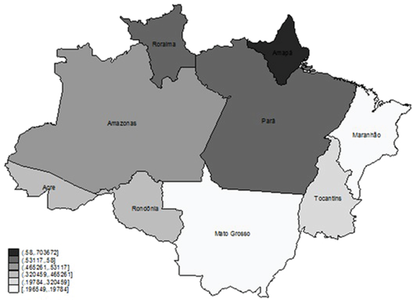
Figure 2. Protected areas in 2010, proportions.

Figure 3. Used land in 2010, proportions.
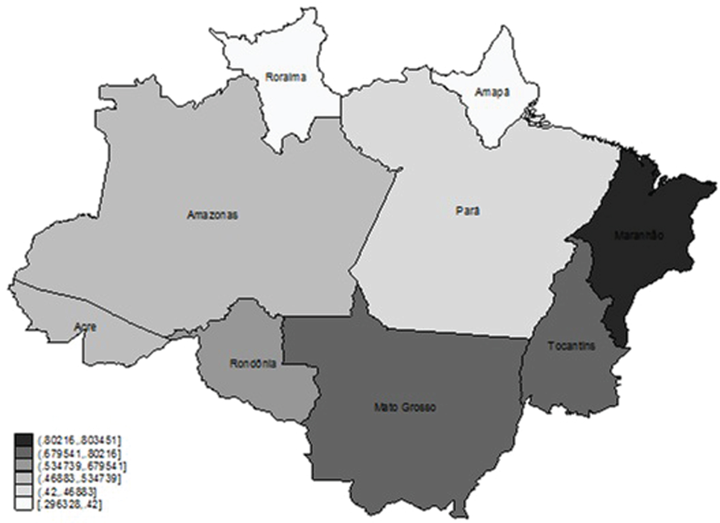
Figure 4. Total minus protected land in 2010, proportions.
3.1 Forestland in the Brazilian Amazon
In figure 1, we provide for each state the available surface of forestland in 2010 as a percentage of the total land of the state. The available forestland is defined as the difference between the total land surface minus the protected areas (figure 2) and the previously converted/used land (figure 3). The data for the total surface and the protected land are taken from Veríssimo et al. (Reference Veríssimo2011), while the data for the converted land are taken from the IBGE census.Footnote 16 Concerning the definition of protected land, we used data provided by Veríssimo et al. (Reference Veríssimo2011). They provide figures relative to ‘indigenous lands’ and ‘protected areas’ in 2010 for the following states: Acre, Amapa, Amazonas, Maranhão, Mato Grosso, Para, Rhodonea, Roraima and Tocantis.
The average surface occupied by both portions amounts to 44 per cent of the total land surface and in our paper we will refer to it as ‘protected areas’.Footnote 17 Therefore, in order to calculate the surface of forestland potentially convertible to agriculture, we must first deduct from the current extent of forestland the surfaces occupied by ‘protected areas’ (see figure 4 for an illustration of the resulting surface). Second, we must also deduct the used land (see figure 1 for an illustration of the resulting surface).
Summarizing the aggregate data, the Brazilian Amazon covers a total area of 5,006,317 km2 including 1,172,580 km2 of land converted to agriculture. Deducting the surface occupied by indigenous lands and protected areas from the current total forestland, we have an area of potentially convertible forestland covering 1,636,251 km2.
Table 2 summarizes our geographical data and shows the area of the states in km2, divided into total protected areas, used land and available land. The columns ‘Area of the state’ and ‘Total protected areas’ are taken from Veríssimo et al. (Reference Veríssimo2011), while the column ‘used land’ is taken from the IBGE census. Finally, the last column is calculated as total area minus the protected and used land. In parentheses, for each column, we show the percentage of each data over the total surface. In detail, in column 3 we show the percentage of the protected areas over the total surface. This percentage corresponds to figure 2. In column 4, we show the percentage of used land out of the total surface and this corresponds to figure 3. In the last column, we show the percentages shown in figure 1, that is the available land out of the total.
Table 2. Protected areas, used land, available land in km2 and in percentage

3.2 Demand for agricultural commodities
Following Börner et al. (Reference Börner2010), we assume that agricultural expansion mirrors forest loss. We estimate the parameters δ and γ of equation (4) by using IBGE data for permanent and temporary crops cultivated in the whole of Brazil. For 60 different crops, we regress their prices with respect to the agricultural land allocated to each specific crop for the period 1994–2000. We obtain the demand functions:
 $$\eqalign{\ln (P_{i,t}) = &12.16 - 0.727\ln (A_{i,t}) \cr & (0.44)\;(0.057),} $$
where the subscripts i and t stand for crop and year considered, respectively. Standard errors are provided in parentheses while the adjusted R2 is equal to 0.33. Using the estimated figures in equation (11) yields γ ≃ 0.727 and δ = exp(12.16) ≃ 190, 786.
3.3 Conversion costs
Concerning the forest conversion cost, c, we follow Bulte et al. (Reference Bulte2002) and set it equal to 0. This assumption can fit a number of situations where, for instance, actual conversion costs are insignificant or are fully covered by benefits from logging. It may also be, as suggested by Leroux et al. (Reference Leroux, Martin and Goeschl2009), quite realistic in the context of ‘slash and burn’ agriculture. Note that, as  ${\lim\nolimits _{c \to 0}}\hat A = \infty $, setting c = 0 implies that the entire forested area available may actually be subject to deforestation, i.e., Â = L. Furthermore, as
  $\lim\nolimits _{c \to 0}{\rm (}A_0/\hat A{\rm )}^\gamma = 0$, the expected long-run growth rate of forest conversion in equation (10) becomes:
 $$\rho \simeq \left\{ {\matrix{ {[(1/2)\sigma ^2 - \alpha ]/\gamma } \hfill & {{\rm for }\;(1/2)\sigma ^2 > \alpha } \hfill \cr 0 \hfill & {{\rm for }\;(1/2)\sigma ^2 \le \alpha } \hfill \cr } } \right..$$
 It is worth stressing that, as  $\lpar A_{0}/\hat{A}\rpar ^{\gamma}<1$ for c > 0, by assuming that conversion costs are null we are potentially providing an overestimation of the actual rate of forest conversion. This implies that the figures provided in the following sections will depict scenarios where the speed of deforestation is higher than it would be in the presence of a positive conversion cost.
3.4 Trend and volatility of forest benefits
As evident in equation (12), both the drift α and the volatility σ of the process that drives the evolution of the forest benefits, i.e., equation (2), are relevant for calibrating the long-run average rate of forest conversion. However, in the literature there is no consensus about the value to be assigned to these parameters, especially as regards the volatility level.
In order to account for the lack of consensus, we proceed as follows. We estimate the parameters α and σ using, as in Conrad (Reference Conrad1997) and Bulte et al. (Reference Bulte2002), tourist arrivals as a proxy for forest benefits. This is needed because time series data concerning the value of the different ES to be included within the forest benefits, i.e., biodiversity conservation, carbon sequestration, watershed control and so on, are not available. Needless to say, since tourist benefits are only a part of total forest benefits, we cannot claim that our estimates are representative of the evolution over time of the entire vector of the ES associated with forest conservation. In order to cope with this limitation, we then propose a comparative static analysis where we use our estimates for defining a benchmark to be compared with other scenarios where the values given to α and σ are taken from previous studies investigating deforestation and evaluating forest benefits.
For estimating α and σ, we use the monthly data provided by the Brazilian Ministry of Tourism on the number of visitors to Brazil in the period from 1989 to 2016 (available on the Ministry website at http://www.turismo.gov.br/). We first calculate, using Stata's sax12 package, the seasonally-adjusted annual growth rate. Then, we run the Dickey-Fuller test to verify if the assumption of a geometric Brownian motion (GBM) for representation of the dynamic of tourist benefits is plausible. The test yields a score of −1.137, which supports our assumption.Footnote 18 Finally, the rounded results for our estimates are α = 0.01 and σ = 0.150.Footnote 19
As mentioned above, the comparative static analysis will be performed using our estimates for α and σ and values given to these two parameters in previous studies. In particular, Bulte et al. (Reference Bulte2002) use α = {0.00, 0.025, 0.05} and σ = {0.00, 0.125} while Engel et al. (Reference Engel2015) use a time series indexed to the returns of transferable permits in the European market with α = 0.00 and σ = {0.01, 0.025}; Brauneis et al. (Reference Brauneis, Mestel and Palan2013) use a carbon price standard deviation of σ = 0.27 and a price process for the CO2 emission allowances with an expected growth rate of α = 0.07. These parameters are based on evidence from different databases and the sensitivity of their model is tested by letting α vary in a range similar to Bulte et al. (Reference Bulte2002), i.e.,  $\alpha\in\lbrack0\semicolon \; 0.14\rsqb \comma \; $ but with higher volatility values, i.e.,
  $\sigma\in\lbrack0.15\semicolon \; 0.45\rsqb .$ To encompass both our benchmark case and most of the values suggested by previous studies, we pick values for the drift parameter within the range α = {0.01, 0.025, 0.05} and values for the volatility parameter within the range σ = {0.15, 0.175, 0.2, 0.225, 0.25}.
Denoting by Θ the value taken by the expected growth rate of g(t), i.e., (1/2)σ 2 − α, and by ρ the rate of conversion, i.e., ρ ≡ Θ/γ, we report in table 3 the expected growth rates corresponding to the combinations ofα and σ satisfying the constraint Θ > 0 and the corresponding values of ρ. We note that, irrespective of the volatility, the rate of conversion ρ is null for α = 0.05.Footnote 20
Table 3. Trend, volatility and corresponding rate of deforestation

When α = 0.025, the rate is positive only for σ = {0.225, 0.25} and null otherwise. Finally, the rate is potentially higher when considering the combinations where α = 0.01. Note also that a reduction in volatility of 10 percent (from σ = 0.250 to σ = 0.150) entails a higher reduction in the annual rate of deforestation from ρ = 2.92 per cent to ρ = 0.17 per cent. Hence, among all these combinations, we choose the cases in bold, which are sufficiently general to include our benchmark case and both cases with low drifts and cases with low volatility.
Bearing this in mind, table 4 summarizes the parameter values that will be used in our numerical analyses.
Table 4. Parameter values

4. Deforestation rate and timing
In table 5 we provide the saturation time, that is, the number of years needed to totally clear the available forestland. This is calculated using equation (12) and considering for Θ = {0.0003, 0.0013, 0.006, 0.0213} where Θ = 0.0013 corresponds to our benchmark case while the other values of Θ correspond to scenarios to be used for our comparative statics. Furthermore, in table 6 we provide the percentage of forestland which, on the basis of the calculated rates of forest conversion, would still be available in 20, 100 and 200 years. The figures concerning the entire Brazilian Amazon are provided in the first row of tables 5 and 6, while in the other rows we provide the figures relative to each of the nine Brazilian states included within its area. For each state, we have assumed that the conversion process has started moving from the extent of land developed before 2010, A 0j, where 0 stands for year 2010 and j indicates the name of the state.
Table 5. Deforestation timing (years) in the Brazilian Amazon and its states
Note: Values for Θ = 0.0003 (σ = 0.225 and α = 0.025), Θ = 0.0013 (σ = 0.150 and α = 0.01), Θ = 0.006 (σ = 0.250 and α = 0.025), Θ = 0.0213 (σ = 0.250 and α = 0.01).
Table 6. Available lands in percentage after 20, 100 and 200 years

Note: Values for Θ = 0.0003 (σ = 0.225 and α = 0.025), Θ = 0.0013 (σ = 0.150 and α = 0.01), Θ = 0.006 (σ = 0.250 and α = 0.025), Θ = 0.0213 (σ = 0.250 and α = 0.01).
The best scenario from the perspective of forest conservation is the scenario where Θ = 0.0003. We note in fact that saturation would take thousands of years. We note also that, as the rates of forest conversion are increasing in Θ, the number of years needed for totally clearing the available forestland drops as Θ increases. This reduction is quite pronounced in the case where Θ = 0.0213. We recall that Θ = 0.0003 may result from the combination of low drift and volatility levels, α = 0.000 and σ = 0.025, respectively, or from the combination of relatively higher levels for both parameters, i.e., α = 0.025 and σ = 0.225. It follows that if any potential future scenario is characterized by these two pairs of values, deforestation is not a threat in the near future.
By comparing columns 4 and 5 of table 5, we are able to isolate the effect of the drift, whereas by comparing columns 3 and 5 (or 2 and 4) the effect of volatility can be clearly identified. According to our simulation, the states that maintain forests longer are Amazonas, Pará and Mato Grosso, while at the opposite end of the scale we find Amapá, Acre, Rondônia and Maranhão.Footnote 21
Another way of looking at the same issue is by determining how much forestland, with respect to the total land, will remain available after a certain period. This should illustrate how dramatic deforestation can be and in which states its impact would be more relevant. We show our results in table 6 for 20, 100 and 200 years.
Let us first consider the case of 200 years with Θ = 0.0003. As shown in table 6, in all the cases considered, after 200 years more than 97 per cent of the available forestland remains in pristine state. In other words, the threat of deforestation is extremely weak. The effect of the drift versus volatility in the value of forest benefits is weak. If we compare column 12 (Θ = 0.006, i.e., α = 0.025 and σ = 0.250) to column 10 (Θ = 0.0003, i.e., α = 0.025 and σ = 0.225), we can isolate the effect of σ on the deforestation rate. We note that while the aggregate average level is not so far from the level in column 10, in column 12 the distribution among states is completely different. Indeed, while in column 10 the percentage of available forestland is homogeneous among states, in column 12 we can identify the states that are more vulnerable. Amapá and Acre will have a percentage of available forestland between 50 and 60 per cent, while Maranhão and Rondônia will maintain a percentage of 68–69 per cent. These percentages increase for Tocantis and Roraima (77–78 per cent) and Mato Grosso and Pará (93–95 per cent) and, finally, forestland will remain almost totally available in Amazon (98 per cent).
The scenario is very different in column 13 of table 6 (Θ = 0.0213, i.e., α = 0.01 and σ = 0.250). This case differs from the previous one (Θ = 0.006) only in the lower drift (0.01 versus 0.025). Therefore, comparing column 13 to column 12, we isolate the effect of α. This case is the worst one, characterized by 5 out of 9 states where forestland is totally exhausted. In contrast, forestland would be, almost totally, conserved in Mato Grosso, Pará and Amazonas (99, 82 and 92 per cent, respectively), while only 20 per cent of available forestland would be kept in Roraima. On average, the available forestland will be lower than 70 per cent with strong asymmetry in the distribution.
The last case (Θ = 0.0013, i.e.,α = 0.01 and σ = 0.150) corresponds to our benchmark case and it is shown in column 11. Comparing this to the previous one (Θ = 0.0213), we isolate the effect of volatility which, as can be immediately seen, is crucial for the definition of the deforestation rate, given that on average, the available forestland will be higher than 97 per cent.
We conclude the analysis by commenting on the percentage of available forestland after 20 and 100 years. After 20 years, only two states (Amapá and Acre) have a percentage of available forestland lower than 96 per cent. Regardless of the volatility and the drift, the majority of the other states have percentages above 96 per cent. For some states the dramatic impact of total deforestation starts materializing after 100 years (Amapá and Acre, with 18 and 32 per cent remaining available forestland, respectively; while Rondônia and Maranhão show a percentage lower than 50 per cent, with Θ = 0.0213), while it concerns the majority of states after 200 years. After 100 years, the effect of volatility (when comparing columns 7 and 9) becomes more evident and only its reduction may deter total deforestation in some states. However, after 200 years, since the rate ρ is positive in any case, total deforestation is unavoidable in some states even in the presence of lower levels of volatility.
5. Conclusions
This article analyzes the long-term rate of forest conversion in the Brazilian Amazon. Based on the models proposed by Bulte et al. (Reference Bulte2002) and Di Corato et al. (Reference Di Corato, Moretto and Vergalli2013), we have calculated the long-run average deforestation rates for nine Brazilian states and we have analyzed the main variables that may accelerate the process.
By using tourist arrivals as a proxy, we estimated the parameters driving the evolution of the value associated with forest benefits. We then performed some comparative static analyses using parameter values taken from previous studies investigating deforestation and the evaluation of forest benefits. In some cases, forest benefits are quantified by looking at the values of transferable permits or emission allowances. This implies that their volatility could also have been affected by policy choices taken in order to regulate the permit markets.
We propose the long-run rate of deforestation as a measure that may reasonably illustrate what we should expect taking into account all the likely conversion paths resulting from: (i) the evolution of the biodiversity value over time; and (ii) the conversion barrier set by equation (8). The analysis of course has limits and one in particular – unfortunately common also to other studies – which is that it is based on the information available today. However, the existence of a steady state is also compatible with recent data from INPE that shows deforestation rates decreasing and increasing in time fluctuating around an ergodic process.
We present the situation of the available forestland after 20, 100 and 200 years. We do this assuming that the demand for agricultural products is the main driver of deforestation and allowing for uncertain benefits from forest conservation. These drivers that push deforestation move antithetically to the forces that lead to conservation, such as the value of benefits related to biodiversity, tourism, carbon sequestration and watershed control. On the one hand, deforestation implies a reduction in environmental services, while on the other hand, it implies an increase in agricultural profits. The struggle of these two opposite values finally drives the net effect of deforestation. Given the role of agriculture in deforestation, we discuss some plausible comparative statics concerning the deforestation rate in the presence of shocks on the elasticity of the demand for agricultural commodities.
The main results of the paper show that the uncertainty surrounding the value attributed to the benefits of biodiversity plays a crucial role in accelerating deforestation. This acceleration is only partially mitigated by a positive growth rate in the value of these benefits. In particular, in our calibration, the results shows that a reduction in the volatility of 10 per cent, with a stable drift, decreases the deforestation rate to about one-fourth, thus maintaining more land forested. These findings suggest that due to the high volatility which, in recent years, has characterized the Emission Trading Systems introduced in some countries, policy makers designing Payments for Environmental Services (PES) schemes should be very cautious when using the emission allowances as a proxy for the value of forest benefits.Footnote 22
It is also shown that the clearing process can be more or less slow depending on the total available land and on the land already developed. It is in fact observed that, in some Brazilian states, forestland is cleared earlier than in others. In general, using the deforestation rates calculated with the data in our possession, we observe that total exhaustion of the forest stock in the short run (20 years) is unlikely, whereas deforestation should start raising concerns in some states when considering a 100-year horizon and definitely becomes a major issue for the majority of the states when considering a 200-year horizon.
We conclude by stressing that potentially relevant extensions of our model could be developed by allowing for uncertain agricultural revenues. This is left to future research.
Acknowledgement
The authors gratefully acknowledge financial support from the University of Padova, grant BIRD 173594.
Appendix A: Proof of Proposition 1
In this section, we study the optimal conversion policy. The value associated with the current land allocation, (A(t), F(t)), is given by:
 $$\eqalign{& V(A(t),g(t)) = \mathop {\max }\limits_{A(s)} E_t\left[ {\int_t^\infty {e^{ - rs}} (W(A(s),g(s)) - cdA)ds} \right] \cr & {\rm s}{\rm .t}{\rm . }dA(s) \ge 0{\rm with }\,A(s) \le \hat A \le L,\;{\rm and }({\rm 2})\;{\rm for\,all\,s},} $$
where r is the constant risk-free interest rate and
 $$[ W(A(t),g(t))=N\lpar A(t)\rpar +({\bar L}-A\lpar t\rpar )g(t)$$
with
 $$N{\rm (}A(t){\rm )} = \mathop \smallint \limits_0^{A(t)} P{\rm (}a{\rm )}da = \delta \displaystyle{{A{(t)}^{1 - \gamma }} \over {1 - \gamma }}.$$
Using standard arguments, we can restate the value function above as:Footnote 23
 $$V(A,g) = \left\{ {W(A,g)dt + \displaystyle{{E_0[V(A,g + dg)]} \over {1 + rdt}}} \right\}.$$
By a straightforward application of Ito's Lemma, equation (A2) can be restated as:
 $$\Gamma V(A,g)=-W(A,g),$$
where Γ is the differential operator: Γ = −r + αp(∂/∂g) + (1/2)σ 2g 2(∂2/∂g 2).
Differentiating (A3) with respect to A, we have:
 $$\Gamma v(A,g)=-w(A,g),$$
where v(A, g) = ∂V(A, g)/∂A and w(A, g) = ∂W(A, g)/∂A.
The solution of equation (A4) takes the functional form:
 $$v(A,g) = m(A,g) + K_1(A)g^{\beta _1} + K_2(A)g^{\beta _2},$$
 where β1 > 1, β2 < 0 are the roots of the characteristic equation  $\Gamma\lpar \beta\rpar =\displaystyle{{1}\over{2}}\sigma^{2}\beta\lpar \beta-1\rpar +\alpha\beta-r=0$, K 1(A), K 2(A) are two constants to be determined and m(A, g) is the particular solution of the non-homogeneous equation. Note that given the current surface, A, allocated to agriculture, m(A, g) represents the expected net present value from converting an additional unit of land. That is:Footnote 24
 $$m(A,g) = E_0\left[ {\int_0^\infty {e^{ - rt}} w(A,g)dt\;} \right] = E_0\left[ {\int_0^\infty {e^{ - rt}} (\delta A^{ - \gamma } - g)dt\;} \right] = \delta \displaystyle{{A^{ - \gamma }} \over r} - \displaystyle{g \over {r - \alpha }}.$$
The boundary conditions for (A5) are
 $$v(A,g^ * (A)) = c,\;v_g(A,g^ * (A)) = 0$$
 $$K_1(A) = 0, K_2(\hat A) = 0.$$
Substituting (A5) into the system (A5a-A5b) yields
 $$\eqalign{& K_2(A)g^{ * \beta _2} + \delta \displaystyle{{A^{ - \gamma }} \over r} - \displaystyle{{g^ * } \over {r - \alpha }} = c \cr & K_2(A)\beta _2g^{ * \beta _2 - 1} - \displaystyle{1 \over {r - \alpha }} = 0.} $$
Solving for g*(A) and K 2(A) we obtain:
 $$\matrix{ {g^ * (A)} \hfill & { = \displaystyle{{\beta _2} \over {\beta _2 - 1}}(r - \alpha )\left[ {{\left( {\displaystyle{{\hat A} \over A}} \right)}^\gamma - 1} \right]c} \hfill \cr } $$
 $$v(A,g) = m(A,g) + \displaystyle{{g^ * (A)} \over {\beta _2\left( {r - \alpha } \right)}}(\displaystyle{g \over {g^ * (A)}})^{\beta _2},$$
where  $\hat{A}=\lpar {\delta}/{rc}\rpar ^{1/\gamma}\ $is the last unit of land for which conversion is worthwhile, i.e.,
  $\delta\hat{A}^{-\gamma}/r=c$.
Appendix B: Proof of Proposition 2
Using equation (8), let us define:
 $$\omega = \displaystyle{g \over {{(\hat A/A)}^\gamma - 1}},\quad {\rm for}\;\omega > \bar \omega = \displaystyle{\beta \over {\beta - 1}}{\rm (}r - \alpha {\rm )}c,$$
 where {ω} is a regulated process in the sense of Harrison (Reference Harrison1985, chap. 2) with  ${\bar \omega}$ as a lower reflecting barrier.
Taking the logarithm on both sides of (B1), we obtain
 $$\ln\omega\ =\ln g-\ln[ e^{\gamma(\ln\hat{A}-\ln A)}-1] .$$
 Using a first-order approximation on the right hand side around the point  $\widetilde{\ln A}\comma \; $ we have
 $$\ln\omega\simeq x_{0}+x_{1}\ln A+\ln g,$$
where
 $$\eqalign{& x_0 = - \left\{ {\ln \left[ {e^{\gamma (\ln \hat A - \widetilde{\ln A})} - 1} \right] + \displaystyle{\gamma \over {1 - e^{ - \gamma (\ln \hat A - \widetilde{\ln A})}}} \widetilde{\ln A}} \right\} \cr & x_1 = \displaystyle{\gamma \over {1 - e^{ - \gamma (\ln \hat A - \widetilde{\ln A})}}}.} $$
By a straightforward application of Ito's lemma, it is easy to show that the process {lnω} evolves according to the same Brownian motion that drives the process {ln g}, i.e.,
 $$d\ln g=\left(\alpha-\displaystyle{{1}\over{2}}\sigma^{2}\right)dt+\sigma dZ.$$
 Following Dixit (Reference Dixit1993: 61), the long-run density function associated with a process {lnω} fluctuating between an upper reflecting barrier, u → ∞, and a lower reflecting barrier,  $\ln{\bar \omega}$, is given by the truncated exponential distribution:
 $$\eqalign{& f{\rm (}\ln \omega {\rm )} = \left\{ {\matrix{ 0 \hfill & {\alpha \ge \displaystyle{1 \over 2}\sigma ^2,} \hfill \cr { - (2\displaystyle{\alpha \over {\sigma ^2}} - 1)e^{(2(\alpha /\sigma ^2) - 1)(\ln \omega - \ln \bar \omega )}} \hfill & {\alpha < \displaystyle{1 \over 2}\sigma ^2.} \hfill \cr } } \right. \cr & {\rm for }\ln \bar \omega {\rm } < \ln \omega < \infty .} $$
 Note that every time the process {lnω} reaches the barrier  $\ln{\bar \omega}$, i.e., when g is sufficiently low, then A increases to prevent {lnω} from passing the barrier.Footnote 25 Hence, using equation (B3), it follows that
 $$d\ln A\simeq-d\ln g/x_{1}.$$
Taking the expected value on both sides of equation (B4) and rearranging, we obtain
 $$\displaystyle{{E\{ d\ln A\} } \over {dt}} = [(1/2)\sigma ^2 - \alpha ]\displaystyle{{1 - e^{ - \gamma (\ln \hat A - \widetilde{\ln A})}} \over \gamma }.$$
 Note that by the monotonicity of the logarithm function, an à must exist such that  $\ln\widetilde{A}=\widetilde{\ln A}$. This implies that the long-run average rate of deforestation can be stated as:
 $$\displaystyle{{E\{ d\ln A\} } \over {dt}} = [(1/2)\sigma ^2 - \alpha ]\displaystyle{{1 - {(\tilde A/\hat A)}^\gamma } \over \gamma }.$$
Equation (10) can then be obtained by setting à = A 0.


