


1 Introduction
In this paper, we derive an evolution equation for the wave envelope of acoustic-gravity (hydroacoustic) waves in a weakly compressible fluid, characterised by depth variations of the sound speed. Our results provide a novel analytical description of the role of the sound speed vertical profile on the propagation of hydroacoustic waves over large spatial and temporal scales.
Recent recordings of underwater acoustic sound associated with the generation of earthquake tsunamis (Levin & Nosov Reference Levin and Nosov2009) and hurricane surges (Wilson & Makris Reference Wilson and Makris2008) have sparked an unprecedented development of analytical and numerical theories to investigate the co-generation of gravity and hydroacoustic (HA) waves by the same source. Such an interest is motivated by HA waves travelling much faster than surface gravity waves, which makes the former excellent forerunners to predict the latter, e.g. to trigger early warning systems for coastal flooding.
Sells (Reference Sells1965), Yamamoto (Reference Yamamoto1982), Levin & Nosov (Reference Levin and Nosov2009) and Stiassnie (Reference Stiassnie2010) were among the first to provide analytical descriptions of tsunamigenic HA waves propagating in a two-dimensional ocean of constant depth. Later, Renzi & Dias (Reference Renzi and Dias2014) extended the analysis to HA waves generated by surface pressure perturbations localised in space and time. Further developments included the effects of bottom elasticity (Eyov et al. Reference Eyov, Klar, Kadri and Stiassnie2013) and two-dimensional depth variations (Kadri Reference Kadri2015). Analytical and numerical models were also devised to understand the motion of HA waves in more complex, three-dimensional scenarios (see Sammarco et al. Reference Sammarco, Cecioni, Bellotti and Abdolali2013; Abdolali et al. Reference Abdolali, Cecioni, Bellotti and Kirby2015a; Abdolali, Kirby & Bellotti Reference Abdolali, Kirby and Bellotti2015b; Cecioni et al. Reference Cecioni, Abdolali, Bellotti and Sammarco2015; Renzi Reference Renzi2017; Mei & Kadri Reference Mei and Kadri2018).
All the above-mentioned models are based upon the simplifying assumption that the speed of sound in water is constant. In reality, the speed of sound in water has spatial variability, as it depends on temperature, salinity and depth (Jensen et al. Reference Jensen, Kuperman, Porter and Schmidt2011). This variability affects the way HA waves propagate in the oceanic waveguide, because the sound speed in the ocean plays the same role as the refractive index in optics. Therefore, using a constant speed profile is not entirely accurate and can lead to appreciable errors in modelling HA wave propagation. Since temperature and salinity also depend on depth, oceanographers have devised idealised sound speed vertical profiles representative of specific oceanic environments, which are a function of the depth coordinate. In deep water, the exponential decrease of stratification with depth suggests the use of an exponential form for the sound speed profile, first devised by Munk (Reference Munk1974) and known as the Munk profile. Such a profile is characterised by the presence of a minimum sound speed below the free surface, which reproduces the features of deep-sound-channel propagation (SOFAR channel; see Jensen et al. (Reference Jensen, Kuperman, Porter and Schmidt2011)) discovered by Ewing & Worzel (Reference Ewing and Worzel1948) during World War II. Indeed, using a numerical model based on the finite-difference method, Jensen et al. (Reference Jensen, Kuperman, Porter and Schmidt2011) showed that the normal-mode shapes are noticeably affected by a vertical variation of the sound speed of the Munk type. However, to the best of our knowledge, no study has been developed to date that investigates this phenomenon analytically.
In this paper we consider the effects of a non-homogeneous sound speed profile on the propagation of HA waves in a two-dimensional, deep-ocean waveguide, over a rigid bottom (Kadri Reference Kadri2016; Abdolali et al. Reference Abdolali, Kadri, Parsons and Kirby2018). We derive an analytical model of HA propagation based on a perturbation expansion of the governing equations, showing that, for a depth-dependent sound speed vertical profile, the frequency and time evolution of the signal change with respect to the constant speed case.
Our results highlight that (i) the depth variability of the sound speed is not generally negligible and (ii) sound speed vertical profiles should be included in HA wave models to ensure a more accurate estimation of the time of arrival of HA waves, especially when these are to be used in practical applications, such as tsunami early warning.
2 Mathematical model
2.1 Governing equations
Let us consider an ocean of constant depth  $h^{\prime }$ and define a Cartesian reference system
  $(x^{\prime },z^{\prime })$ with the
  $x^{\prime }$ axis lying on the undisturbed free-surface level and the
  $z^{\prime }$ axis pointing upwards. Primes indicate physical variables. We assume that HA waves are generated by a distant source (e.g. an earthquake) in the deep ocean. For deep-ocean waveguides the sound speed can be considered range-independent:
  $c^{\prime }=c^{\prime }(z^{\prime })$ (see Jensen et al. Reference Jensen, Kuperman, Porter and Schmidt2011).
Let us express the total water density  $\unicode[STIX]{x1D70C}^{\prime }$ and pressure
  $p^{\prime }$ as follows (Levin & Nosov Reference Levin and Nosov2009; Jensen et al. Reference Jensen, Kuperman, Porter and Schmidt2011; Renzi & Dias Reference Renzi and Dias2014):
 $$\begin{eqnarray}\displaystyle \unicode[STIX]{x1D70C}^{\prime }=\unicode[STIX]{x1D70C}_{D}^{\prime }+\unicode[STIX]{x1D70C}_{0}^{\prime },\quad p^{\prime }=p_{D}^{\prime }+p_{0}^{\prime }, & & \displaystyle\end{eqnarray}$$
 where  $\unicode[STIX]{x1D70C}_{D}^{\prime }$ and
  $p_{D}^{\prime }$ represent the dynamical quantities depending on space and time
  $t^{\prime }$,
  $\unicode[STIX]{x1D70C}_{0}^{\prime }=1030~\text{kg}~\text{m}^{-3}$ is the static water density, while
  $p_{0}^{\prime }$ is the hydrostatic ambient pressure in the absence of acoustic disturbances. Since dynamic processes in acoustic waves are assumed to be adiabatic, if we consider small fluctuations of both pressure and density, i.e.
  $\unicode[STIX]{x1D70C}_{D}^{\prime }\ll \unicode[STIX]{x1D70C}_{0}^{\prime }$,
  $p_{D}^{\prime }\ll p_{0}^{\prime }$, the continuity equation and the Euler equation for a weakly compressible flow can be written, respectively, as (Levin & Nosov Reference Levin and Nosov2009)
 $$\begin{eqnarray}\displaystyle & \displaystyle \unicode[STIX]{x1D70C}_{D_{t^{\prime }}}^{\prime }+\unicode[STIX]{x1D6F7}_{x^{\prime }}^{\prime }\unicode[STIX]{x1D70C}_{D_{x^{\prime }}}^{\prime }+\unicode[STIX]{x1D6F7}_{z^{\prime }}^{\prime }\unicode[STIX]{x1D70C}_{D_{z^{\prime }}}^{\prime }+\unicode[STIX]{x1D70C}_{0}^{\prime }(\unicode[STIX]{x1D6F7}_{x^{\prime }x^{\prime }}^{\prime }+\unicode[STIX]{x1D6F7}_{z^{\prime }z^{\prime }}^{\prime })=0, & \displaystyle\end{eqnarray}$$
 $$\begin{eqnarray}\displaystyle & \displaystyle -\frac{p_{D}^{\prime }}{\unicode[STIX]{x1D70C}_{0}^{\prime }}=\unicode[STIX]{x1D6F7}_{t^{\prime }}^{\prime }+\frac{{\unicode[STIX]{x1D6F7}^{\prime }}_{x^{\prime }}^{2}+{\unicode[STIX]{x1D6F7}^{\prime }}_{z^{\prime }}^{2}}{2}, & \displaystyle\end{eqnarray}$$
 where  $\unicode[STIX]{x1D6F7}^{\prime }(x^{\prime },z^{\prime },t^{\prime })$ is the velocity potential defined in the fluid domain
  $\unicode[STIX]{x1D6FA}(x^{\prime },z^{\prime })$. Furthermore, the equation of state reads (Brekhovskikh & Godin Reference Brekhovskikh and Godin1992)
 $$\begin{eqnarray}\displaystyle {c^{\prime }}^{2}(\unicode[STIX]{x1D70C}_{D_{t^{\prime }}}^{\prime }+\unicode[STIX]{x1D6F7}_{x^{\prime }}^{\prime }\unicode[STIX]{x1D70C}_{D_{x^{\prime }}}^{\prime }+\unicode[STIX]{x1D6F7}_{z^{\prime }}^{\prime }\unicode[STIX]{x1D70C}_{D_{z^{\prime }}}^{\prime })=p_{D_{t^{\prime }}}^{\prime }+\unicode[STIX]{x1D6F7}_{x^{\prime }}^{\prime }p_{D_{x^{\prime }}}^{\prime }+\unicode[STIX]{x1D6F7}_{z^{\prime }}^{\prime }p_{D_{z^{\prime }}}^{\prime }-\unicode[STIX]{x1D70C}_{0}^{\prime }g^{\prime }\unicode[STIX]{x1D6F7}_{z^{\prime }}^{\prime }, & & \displaystyle\end{eqnarray}$$
 where  $g^{\prime }$ is the acceleration due to gravity. Substitution of (2.4) in (2.2) and usage of the Euler equation (2.3) gives the following governing equation:
 $$\begin{eqnarray}\displaystyle & & \displaystyle \unicode[STIX]{x1D6F7}_{t^{\prime }t^{\prime }}^{\prime }-{c^{\prime }}^{2}(\unicode[STIX]{x1D6F7}_{x^{\prime }x^{\prime }}^{\prime }+\unicode[STIX]{x1D6F7}_{z^{\prime }z^{\prime }}^{\prime })+{\textstyle \frac{1}{2}}[\unicode[STIX]{x1D6F7}_{x^{\prime }}^{\prime }({\unicode[STIX]{x1D6F7}^{\prime }}_{x^{\prime }}^{2}+{\unicode[STIX]{x1D6F7}^{\prime }}_{z^{\prime }}^{2})_{x^{\prime }}+\unicode[STIX]{x1D6F7}_{z^{\prime }}^{\prime }({\unicode[STIX]{x1D6F7}^{\prime }}_{x^{\prime }}^{2}+{\unicode[STIX]{x1D6F7}^{\prime }}_{z^{\prime }}^{2})_{z^{\prime }}]\nonumber\\ \displaystyle & & \displaystyle \quad +\,({\unicode[STIX]{x1D6F7}^{\prime }}_{x^{\prime }}^{2}+{\unicode[STIX]{x1D6F7}^{\prime }}_{z^{\prime }}^{2})_{t^{\prime }}+g^{\prime }\unicode[STIX]{x1D6F7}_{z^{\prime }}^{\prime }=0.\end{eqnarray}$$
 We remark that the governing equation (2.5) is similar to that already obtained by Longuet-Higgins (Reference Longuet-Higgins1950) except for the depth-dependent function  $c^{\prime }(z^{\prime })$. The variation of
  $c^{\prime }(z^{\prime })$ with respect to the constant value
  $c_{0}^{\prime }=1500~\text{m}~\text{s}^{-1}$ can be generally written as (Jensen et al. Reference Jensen, Kuperman, Porter and Schmidt2011)
 $$\begin{eqnarray}\displaystyle c^{\prime }=c_{0}^{\prime }[1+\unicode[STIX]{x1D716}f(z^{\prime })], & & \displaystyle\end{eqnarray}$$
 where  $\unicode[STIX]{x1D716}\ll 1$ is a small non-dimensional constant, while
  $f^{\prime }(z^{\prime })$ represents the variation along
  $z^{\prime }$. We require that
  $f^{\prime }(z^{\prime })$ be a continuous and bounded function (Bender & Orszag Reference Bender and Orszag1999). Assume that the pressure on the free surface
  $z^{\prime }=\unicode[STIX]{x1D701}^{\prime }$ is null, hence the mixed boundary condition on the free surface is given by (Mei, Stiassnie & Yue Reference Mei, Stiassnie and Yue2005)
 $$\begin{eqnarray}\displaystyle \unicode[STIX]{x1D6F7}_{t^{\prime }t^{\prime }}^{\prime }+g^{\prime }\unicode[STIX]{x1D6F7}_{z^{\prime }}^{\prime }+({\unicode[STIX]{x1D6F7}^{\prime }}_{x^{\prime }}^{2}+{\unicode[STIX]{x1D6F7}^{\prime }}_{z^{\prime }}^{2})_{t^{\prime }}+{\textstyle \frac{1}{2}}[\unicode[STIX]{x1D6F7}_{x^{\prime }}^{\prime }({\unicode[STIX]{x1D6F7}^{\prime }}_{x^{\prime }}^{2}+{\unicode[STIX]{x1D6F7}^{\prime }}_{z^{\prime }}^{2})_{x^{\prime }}+\unicode[STIX]{x1D6F7}_{z^{\prime }}^{\prime }({\unicode[STIX]{x1D6F7}^{\prime }}_{x^{\prime }}^{2}+{\unicode[STIX]{x1D6F7}^{\prime }}_{z^{\prime }}^{2})_{z^{\prime }}]=0,\quad z^{\prime }=\unicode[STIX]{x1D701}^{\prime }, & & \displaystyle \nonumber\\ \displaystyle & & \displaystyle\end{eqnarray}$$
 where  $g^{\prime }$ is the acceleration due to gravity. Finally, the no-flux condition at the rigid bottom requires
 $$\begin{eqnarray}\displaystyle \unicode[STIX]{x1D6F7}_{z^{\prime }}^{\prime }=0,\quad z^{\prime }=-h^{\prime }. & & \displaystyle\end{eqnarray}$$
2.2 Multiple-scale analysis
Let us introduce the following non-dimensional quantities (Mei et al. Reference Mei, Stiassnie and Yue2005; Michele, Sammarco & d’Errico Reference Michele, Sammarco and d’Errico2018; Michele & Renzi Reference Michele and Renzi2019; Michele, Renzi & Sammarco Reference Michele, Renzi and Sammarco2019)
 $$\begin{eqnarray}\displaystyle \left.\begin{array}{@{}l@{}}(x,z)=2\unicode[STIX]{x03C0}(x^{\prime },z^{\prime })/\unicode[STIX]{x1D706}^{\prime },\quad \unicode[STIX]{x1D6F7}=2\unicode[STIX]{x03C0}\unicode[STIX]{x1D6F7}^{\prime }/(A^{\prime }\unicode[STIX]{x1D714}^{\prime }\unicode[STIX]{x1D706}^{\prime }),\quad \unicode[STIX]{x1D701}=\unicode[STIX]{x1D701}^{\prime }/A^{\prime },\quad c_{0}=2\unicode[STIX]{x03C0}c_{0}^{\prime }/(\unicode[STIX]{x1D714}^{\prime }\unicode[STIX]{x1D706}^{\prime }),\\ t=t^{\prime }\unicode[STIX]{x1D714}^{\prime },\quad h=2\unicode[STIX]{x03C0}h^{\prime }/\unicode[STIX]{x1D706}^{\prime },\quad G=2\unicode[STIX]{x03C0}g^{\prime }/({\unicode[STIX]{x1D714}^{\prime }}^{2}\unicode[STIX]{x1D706}^{\prime }),\quad \unicode[STIX]{x1D6FF}=2\unicode[STIX]{x03C0}A^{\prime }/\unicode[STIX]{x1D706}^{\prime }.\end{array}\right\}\quad & & \displaystyle\end{eqnarray}$$
Using the Euler equation (2.3) and the dimensionless variables (2.9), equation (2.5) becomes
 $$\begin{eqnarray}\displaystyle & & \displaystyle \unicode[STIX]{x1D6F7}_{tt}-c_{0}^{2}(1+\unicode[STIX]{x1D716}f)^{2}(\unicode[STIX]{x1D6F7}_{xx}+\unicode[STIX]{x1D6F7}_{zz})+{\textstyle \frac{1}{2}}\unicode[STIX]{x1D6FF}^{2}[\unicode[STIX]{x1D6F7}_{x}(\unicode[STIX]{x1D6F7}_{x}^{2}+\unicode[STIX]{x1D6F7}_{z}^{2})_{x}+\unicode[STIX]{x1D6F7}_{z}(\unicode[STIX]{x1D6F7}_{x}^{2}+\unicode[STIX]{x1D6F7}_{z}^{2})_{z}]\nonumber\\ \displaystyle & & \displaystyle \quad +\,\unicode[STIX]{x1D6FF}(\unicode[STIX]{x1D6F7}_{x}^{2}+\unicode[STIX]{x1D6F7}_{z}^{2})_{t}+G\unicode[STIX]{x1D6F7}_{z}=0.\end{eqnarray}$$
The mixed boundary condition on the free surface (2.7) gives
 $$\begin{eqnarray}\displaystyle \unicode[STIX]{x1D6F7}_{tt}+G\unicode[STIX]{x1D6F7}_{z}+\unicode[STIX]{x1D6FF}(\unicode[STIX]{x1D6F7}_{x}^{2}+\unicode[STIX]{x1D6F7}_{z}^{2})_{t}+{\textstyle \frac{1}{2}}\unicode[STIX]{x1D6FF}^{2}[\unicode[STIX]{x1D6F7}_{x}(\unicode[STIX]{x1D6F7}_{x}^{2}+\unicode[STIX]{x1D6F7}_{z}^{2})_{x}+\unicode[STIX]{x1D6F7}_{z}(\unicode[STIX]{x1D6F7}_{x}^{2}+\unicode[STIX]{x1D6F7}_{z}^{2})_{z}]=0,\quad z=\unicode[STIX]{x1D6FF}\unicode[STIX]{x1D701},\quad & & \displaystyle\end{eqnarray}$$
while the non-dimensional no-flux condition at the bottom is given by
 $$\begin{eqnarray}\displaystyle \unicode[STIX]{x1D6F7}_{z}=0,\quad z=-h. & & \displaystyle\end{eqnarray}$$
 Now consider the physical scales of the problem. The typical maximum amplitude of tsunamigenic HA waves is  $A^{\prime }\sim 10^{-2}~\text{m}$ (Kadri & Stiassnie Reference Kadri and Stiassnie2012), whereas the wavelength is
  $\unicode[STIX]{x1D706}^{\prime }\sim 10^{4}~\text{m}$ and the angular frequency is
  $\unicode[STIX]{x1D714}^{\prime }\sim 1~\text{rad}~\text{s}^{-1}$ (see Stiassnie Reference Stiassnie2010; Cecioni et al. Reference Cecioni, Abdolali, Bellotti and Sammarco2015; Renzi Reference Renzi2017). Furthermore, the sound speed parameter in (2.6) is
  $\unicode[STIX]{x1D716}\sim 10^{-1}$ (see Jensen et al. Reference Jensen, Kuperman, Porter and Schmidt2011), thus
  $O(G)=O(\unicode[STIX]{x1D716}^{2})$, while the nonlinearity parameter
  $\unicode[STIX]{x1D6FF}\sim 10^{-6}$. Since
  $\unicode[STIX]{x1D6FF}$ is very small, the non-dimensional governing equation (2.10) and the free-surface boundary condition (2.11) simplify as follows:
 $$\begin{eqnarray}\displaystyle & \displaystyle \unicode[STIX]{x1D6F7}_{tt}-c_{0}^{2}(1+\unicode[STIX]{x1D716}f)^{2}(\unicode[STIX]{x1D6F7}_{xx}+\unicode[STIX]{x1D6F7}_{zz})+G\unicode[STIX]{x1D6F7}_{z}+O(\unicode[STIX]{x1D716}^{3})=0, & \displaystyle\end{eqnarray}$$
 $$\begin{eqnarray}\displaystyle & \displaystyle \unicode[STIX]{x1D6F7}_{tt}+G\unicode[STIX]{x1D6F7}_{z}+O(\unicode[STIX]{x1D716}^{3})=0,\quad z=0. & \displaystyle\end{eqnarray}$$
Let us now introduce the following expansion of the non-dimensional velocity potential:
 $$\begin{eqnarray}\displaystyle \unicode[STIX]{x1D6F7} & = & \displaystyle \unicode[STIX]{x1D6F7}_{1}(x,x_{1},x_{2},z,t,t_{1},t_{2})+\unicode[STIX]{x1D716}\unicode[STIX]{x1D6F7}_{2}(x,x_{1},x_{2},z,t,t_{1},t_{2})\nonumber\\ \displaystyle & & \displaystyle +\,\unicode[STIX]{x1D716}^{2}\unicode[STIX]{x1D6F7}_{3}(x,x_{1},x_{2},z,t,t_{1},t_{2})+O(\unicode[STIX]{x1D716}^{3}),\end{eqnarray}$$
 where  $t_{1}=\unicode[STIX]{x1D716}t$ and
  $t_{2}=\unicode[STIX]{x1D716}^{2}t$ denote two slow time scales of the amplitude evolution, while
  $x_{1}=\unicode[STIX]{x1D716}x$ and
  $x_{2}=\unicode[STIX]{x1D716}^{2}x$ are two slow spatial scales that account for slow modulation along the
  $x$ coordinate.
Since  $\unicode[STIX]{x1D716}\ll 1$, the perturbation expansion method is a valid approach to obtain an approximate solution of the initial mathematical problem. We remark that, in the case of generalised sound speed profiles characterised by large parameters
  $\unicode[STIX]{x1D716}\geqslant 1$, the scales (2.9) fail and different approaches should be considered (Xu et al. Reference Xu, Lin, Liao and Stiassnie2012; Liao, Xu & Stiassnie Reference Liao, Xu and Stiassnie2016).
Substitution of expansion (2.15) for the velocity potential  $\unicode[STIX]{x1D6F7}$ in (2.13) yields for
  $n=1,2,3,$ the governing equation
 $$\begin{eqnarray}\displaystyle \unicode[STIX]{x1D6F7}_{n_{tt}}-c_{0}^{2}(\unicode[STIX]{x1D6F7}_{n_{xx}}+\unicode[STIX]{x1D6F7}_{n_{zz}})={\mathcal{F}}_{n},\quad \text{in }\unicode[STIX]{x1D6FA}, & & \displaystyle\end{eqnarray}$$
where the forcing terms are given by
 $$\begin{eqnarray}\displaystyle {\mathcal{F}}_{1}=0,\quad {\mathcal{F}}_{2}=-2\unicode[STIX]{x1D6F7}_{1_{tt_{1}}}+2c_{0}^{2}\unicode[STIX]{x1D6F7}_{1_{xx_{1}}}+2c_{0}^{2}\,f(\unicode[STIX]{x1D6F7}_{1_{xx}}+\unicode[STIX]{x1D6F7}_{1_{zz}}), & & \displaystyle\end{eqnarray}$$
 $$\begin{eqnarray}\displaystyle {\mathcal{F}}_{3} & = & \displaystyle -2\unicode[STIX]{x1D6F7}_{2_{tt_{1}}}-\unicode[STIX]{x1D6F7}_{1_{t_{1}t_{1}}}-2\unicode[STIX]{x1D6F7}_{1_{tt_{2}}}-\frac{G}{\unicode[STIX]{x1D716}^{2}}\unicode[STIX]{x1D6F7}_{1_{z}}\nonumber\\ \displaystyle & & \displaystyle +\,c_{0}^{2}[f^{2}(\unicode[STIX]{x1D6F7}_{1_{xx}}+\unicode[STIX]{x1D6F7}_{1_{zz}})+2f(\unicode[STIX]{x1D6F7}_{2_{xx}}+\unicode[STIX]{x1D6F7}_{2_{zz}})+4f\unicode[STIX]{x1D6F7}_{1_{xx_{1}}}+2\unicode[STIX]{x1D6F7}_{2_{xx_{1}}}+\unicode[STIX]{x1D6F7}_{1_{x_{1}x_{1}}}+2\unicode[STIX]{x1D6F7}_{1_{xx_{2}}}].\nonumber\\ \displaystyle & & \displaystyle\end{eqnarray}$$
The boundary condition on the free surface is
 $$\begin{eqnarray}\displaystyle \unicode[STIX]{x1D6F7}_{n_{tt}}={\mathcal{G}}_{n},\quad z=0, & & \displaystyle\end{eqnarray}$$
where
 $$\begin{eqnarray}\displaystyle {\mathcal{G}}_{1}=0,\quad {\mathcal{G}}_{2}=-2\unicode[STIX]{x1D6F7}_{1_{tt_{1}}},\quad {\mathcal{G}}_{3}=-2\unicode[STIX]{x1D6F7}_{1_{tt_{2}}}-2\unicode[STIX]{x1D6F7}_{2_{tt_{1}}}-\unicode[STIX]{x1D6F7}_{1_{t_{1}t_{1}}}-\frac{G}{\unicode[STIX]{x1D716}^{2}}\unicode[STIX]{x1D6F7}_{1_{z}}, & & \displaystyle\end{eqnarray}$$
while the homogeneous no-flux boundary condition at the horizontal rigid bottom reads
 $$\begin{eqnarray}\displaystyle \unicode[STIX]{x1D6F7}_{n_{z}}=0,\quad z=-h. & & \displaystyle\end{eqnarray}$$
 Now let us formulate the mathematical problem for a generic frequency  $\unicode[STIX]{x1D714}$. Since the boundary-value problem given by (2.12)–(2.14) is linear, we return to physical variables except for
  $x_{1}$,
  $x_{2}$,
  $t_{1}$ and
  $t_{2}$, omit the primes for convenience and assume the following harmonic expansion:
 $$\begin{eqnarray}\displaystyle \unicode[STIX]{x1D6F7}_{n}=\unicode[STIX]{x1D719}_{n}\text{e}^{-\text{i}\unicode[STIX]{x1D714}t}+\ast , & & \displaystyle\end{eqnarray}$$
 where the symbol  $\ast$ indicates the complex conjugate. Having obtained the governing equations at each order
  $n$, we can now investigate the evolution of HA waves.
2.3 Leading-order solution
The leading-order solution outgoing from a source at  $x\rightarrow -\infty$ is
 $$\begin{eqnarray}\displaystyle \unicode[STIX]{x1D719}_{1}=\mathop{\sum }_{m=0}^{\infty }\unicode[STIX]{x1D719}_{1m}=\mathop{\sum }_{m=0}^{\infty }\text{e}^{\text{i}k_{m}x}\unicode[STIX]{x1D713}_{1m}=\mathop{\sum }_{m=0}^{\infty }\text{e}^{\text{i}k_{m}x}{\mathcal{A}}_{m}(x_{1},x_{2},t_{1},t_{2})\sin \unicode[STIX]{x1D6FD}_{m}z, & & \displaystyle\end{eqnarray}$$
where the eigenvalues are given by
 $$\begin{eqnarray}\displaystyle \unicode[STIX]{x1D6FD}_{m}=\frac{1}{h}\left(\frac{\unicode[STIX]{x03C0}}{2}+m\unicode[STIX]{x03C0}\right),\quad k_{m}=\sqrt{\frac{\unicode[STIX]{x1D714}^{2}}{c_{0}^{2}}-\unicode[STIX]{x1D6FD}_{m}^{2}},\quad m=0,1,\ldots , & & \displaystyle\end{eqnarray}$$
 while  ${\mathcal{A}}_{m}$ represents the amplitude of the
  $m$th HA normal mode depending on the slow variables. In the following we will consider only propagating modes, for which
  $k_{m}^{2}>0$. Furthermore, since the problem is linear, we will assume that the evolution of each HA wave does not involve mode coupling (adiabatic approximation (see Jensen et al. Reference Jensen, Kuperman, Porter and Schmidt2011)).
2.4 Second-order solution
Expanding the second-order velocity potential
 $$\begin{eqnarray}\displaystyle \unicode[STIX]{x1D719}_{2}=\mathop{\sum }_{m=0}^{\infty }\unicode[STIX]{x1D719}_{2m}=\mathop{\sum }_{m=0}^{\infty }\text{e}^{\text{i}k_{m}x}\unicode[STIX]{x1D713}_{2m}, & & \displaystyle\end{eqnarray}$$
 we obtain the following governing equation for  $\unicode[STIX]{x1D713}_{2m}$ forced by the first-order solution:
 $$\begin{eqnarray}\displaystyle \unicode[STIX]{x1D713}_{2m_{zz}}+\unicode[STIX]{x1D713}_{2m}\unicode[STIX]{x1D6FD}_{m}^{2}=2\sin \unicode[STIX]{x1D6FD}_{m}z\left(-\frac{\text{i}\unicode[STIX]{x1D714}^{2}{\mathcal{A}}_{m_{t_{1}}}}{c_{0}^{2}}-\frac{\text{i}k_{m}{\mathcal{A}}_{m_{x_{1}}}}{\unicode[STIX]{x1D706}}+\frac{f\unicode[STIX]{x1D714}^{2}{\mathcal{A}}_{m}}{c_{0}^{2}}\right), & & \displaystyle\end{eqnarray}$$
and the respective boundary conditions on the free surface and at the bottom
 $$\begin{eqnarray}\displaystyle \unicode[STIX]{x1D713}_{2m}=0\quad \text{at }z=0,\quad \text{and}\quad \unicode[STIX]{x1D713}_{2m_{z}}=0\quad \text{at }z=-h. & & \displaystyle\end{eqnarray}$$
 Since  $\unicode[STIX]{x1D713}_{1m}$ solves the homogeneous problem at the leading order, a solvability condition must be applied to
  $\unicode[STIX]{x1D713}_{1m}$ and
  $\unicode[STIX]{x1D713}_{2m}$ to avoid secularity. Green’s theorem gives
 $$\begin{eqnarray}\displaystyle {\mathcal{A}}_{m_{t_{1}}}\frac{\unicode[STIX]{x1D714}^{2}}{c_{0}^{2}}+{\mathcal{A}}_{m_{x_{1}}}\frac{k_{m}}{\unicode[STIX]{x1D706}}+{\mathcal{A}}_{m}\frac{2\text{i}\unicode[STIX]{x1D714}^{2}}{hc_{0}^{2}}\int _{-h}^{0}f\sin ^{2}\unicode[STIX]{x1D6FD}_{m}z\,\text{d}z=0. & & \displaystyle\end{eqnarray}$$
The general solution of the latter equation is readily given by (Hildebrand Reference Hildebrand1962)
 $$\begin{eqnarray}\displaystyle {\mathcal{A}}_{m}={\mathcal{A}}_{m}\left(x_{1}-t_{1}\frac{C_{gm}}{\unicode[STIX]{x1D714}\unicode[STIX]{x1D706}}\right)\exp \left(-\frac{2\text{i}\unicode[STIX]{x1D714}^{2}I_{0m}\unicode[STIX]{x1D706}x_{1}}{hc_{0}^{2}k_{m}}\right), & & \displaystyle\end{eqnarray}$$
where
 $$\begin{eqnarray}\displaystyle I_{0m}=\int _{-h}^{0}f\sin ^{2}\unicode[STIX]{x1D6FD}_{m}z\,\text{d}z, & & \displaystyle\end{eqnarray}$$
 while  $C_{gm}$ is the group velocity for the
  $m$th HA mode, defined by
 $$\begin{eqnarray}\displaystyle C_{gm}=\frac{\text{d}\unicode[STIX]{x1D714}}{\text{d}k_{m}}=\frac{k_{m}c_{0}^{2}}{\unicode[STIX]{x1D714}}. & & \displaystyle\end{eqnarray}$$
 The solution (2.29) is valid until  $x_{1}$ and
  $t_{1}$ become both of order
  $O(1)$. Now substitute (2.29) into (2.23) and transform
  $x_{1}$ and
  $t_{1}$ back to physical variables via (2.9). Using
  $x=C_{gm}t$ reveals that each modal component of the harmonic decomposition (2.22) is, at the leading order,
 $$\begin{eqnarray}\displaystyle \unicode[STIX]{x1D6F7}_{1m}=\unicode[STIX]{x1D719}_{1m}\text{e}^{-\text{i}\unicode[STIX]{x1D714}t}+\ast ={\mathcal{A}}_{m}(0)\exp \left[-\text{i}\left(\unicode[STIX]{x1D714}-C_{gm}k_{m}+\frac{2\unicode[STIX]{x1D716}\unicode[STIX]{x1D714}I_{0m}}{h}\right)t\right]\sin \unicode[STIX]{x1D6FD}_{m}z+\ast .\quad & & \displaystyle\end{eqnarray}$$
 Physically, to an observer moving with the envelope at the group velocity  $x/t=C_{gm}$, the apparent frequency of the wave signal propagating within the envelope is
 $$\begin{eqnarray}\displaystyle \tilde{\unicode[STIX]{x1D714}}_{m}=\unicode[STIX]{x1D714}\left(1+2\unicode[STIX]{x1D716}\frac{I_{0m}}{h}\right)-C_{gm}k_{m}. & & \displaystyle\end{eqnarray}$$
 Note that, for a constant speed profile, the apparent frequency becomes  $\tilde{\unicode[STIX]{x1D714}}_{m}=\unicode[STIX]{x1D714}[1-C_{gm}(k_{m}/\unicode[STIX]{x1D714})]$. The latter naturally results from the Doppler effect associated with the observer moving at the group velocity away from a stationary source that emits waves propagating at the phase speed
  $\unicode[STIX]{x1D714}/k_{m}$. On the other hand, for a variable sound speed vertical profile the frequency grows (reduces) by a term proportional to
  $\unicode[STIX]{x1D716}|I_{0m}|/h$, if
  $I_{0m}>0$ (
 ${<}0$), as shown by (2.33). This in turn increases (decreases) the apparent frequency
  $\tilde{\unicode[STIX]{x1D714}}_{m}$. Furthermore, if
 $$\begin{eqnarray}\displaystyle I_{0m}=-\frac{(\unicode[STIX]{x03C0}/2+m\unicode[STIX]{x03C0})^{2}c_{0}^{2}}{2\unicode[STIX]{x1D716}\unicode[STIX]{x1D714}^{2}h}, & & \displaystyle\end{eqnarray}$$
 the apparent frequency  $\tilde{\unicode[STIX]{x1D714}}_{m}=0$ and the signal would be constant in time to an observer moving at the group velocity. Hence, in principle, the dynamics would be non-dispersive. This can be possible for large frequencies and specific sound speed vertical profiles for which
  $f(z)<0$ over much of the depth, like in the Arctic (Jensen et al. Reference Jensen, Kuperman, Porter and Schmidt2011).
Moving to the second-order problem, the method of variation of parameters allows us to find the solution of the forced differential equation (2.26) (see Hildebrand Reference Hildebrand1962). The homogeneous solution coincides with  $\unicode[STIX]{x1D713}_{1m}$; thus it can be included in the expression for the velocity potential at the leading order. Consequently, the
  $m$th component of the second-order velocity potential
  $\unicode[STIX]{x1D713}_{2m}$ is only given by the particular solution, i.e.
 $$\begin{eqnarray}\displaystyle \unicode[STIX]{x1D713}_{2m}=\frac{\text{i}(h+z)\cos \unicode[STIX]{x1D6FD}_{m}z}{\unicode[STIX]{x1D6FD}_{m}}\left({\mathcal{A}}_{m_{t_{1}}}\frac{\unicode[STIX]{x1D714}^{2}}{c_{0}^{2}}+{\mathcal{A}}_{m_{x_{1}}}\frac{k_{m}}{\unicode[STIX]{x1D706}}\right)+{\mathcal{A}}_{m}\frac{2\unicode[STIX]{x1D714}^{2}F_{m}(z)}{c_{0}^{2}\unicode[STIX]{x1D6FD}_{m}}, & & \displaystyle\end{eqnarray}$$
 where the function  $F_{m}(z)$ has the expression
 $$\begin{eqnarray}\displaystyle F_{m}(z)=\int _{-h}^{z}f(u)\sin \unicode[STIX]{x1D6FD}_{m}u\sin [\unicode[STIX]{x1D6FD}_{m}(z-u)]\,\text{d}u. & & \displaystyle\end{eqnarray}$$
Finally, substitution of (2.28) in (2.35) yields
 $$\begin{eqnarray}\displaystyle \unicode[STIX]{x1D713}_{2m}={\mathcal{A}}_{m}\frac{2\unicode[STIX]{x1D714}^{2}}{c_{0}^{2}\unicode[STIX]{x1D6FD}_{m}}\left[\frac{I_{0m}(h+z)\cos \unicode[STIX]{x1D6FD}_{m}z}{h}+F_{m}(z)\right]\!. & & \displaystyle\end{eqnarray}$$
 Note that the potential  $\unicode[STIX]{x1D713}_{2m}$ is a peculiar signature of the variable sound speed vertical profile
  $c$ and does not exist for constant
  $c=c_{0}$. Indeed, in that case
  $I_{0m}=F_{m}=0$.
2.5 Third-order problem and evolution equation
Let us use the following fast-coordinate expansion for the third-order potential  $\unicode[STIX]{x1D719}_{3}$,
 $$\begin{eqnarray}\displaystyle \unicode[STIX]{x1D719}_{3}=\mathop{\sum }_{m=0}^{\infty }\text{e}^{\text{i}k_{m}x}\unicode[STIX]{x1D713}_{3m}(z). & & \displaystyle\end{eqnarray}$$
 The governing equation for  $\unicode[STIX]{x1D713}_{3m}$ is then given by
 $$\begin{eqnarray}\displaystyle \unicode[STIX]{x1D713}_{3m_{zz}}+\unicode[STIX]{x1D713}_{3m}\unicode[STIX]{x1D6FD}_{m}^{2} & = & \displaystyle \frac{(h+z)\cos \unicode[STIX]{x1D6FD}_{m}z}{\unicode[STIX]{x1D6FD}_{m}}\left[\frac{2\unicode[STIX]{x1D714}^{2}}{c_{0}^{2}}\left({\mathcal{A}}_{m_{t_{1}t_{1}}}\frac{\unicode[STIX]{x1D714}^{2}}{c_{0}^{2}}+{\mathcal{A}}_{m_{x_{1}t_{1}}}\frac{k_{m}}{\unicode[STIX]{x1D706}}\right)\right.\nonumber\\ \displaystyle & & \displaystyle +\left.\frac{2\text{i}\unicode[STIX]{x1D714}^{2}f}{c_{0}^{2}}\left({\mathcal{A}}_{m_{t_{1}}}\frac{\unicode[STIX]{x1D714}^{2}}{c_{0}^{2}}+{\mathcal{A}}_{m_{x_{1}}}\frac{k_{m}}{\unicode[STIX]{x1D706}}\right)+\frac{2k_{m}}{\unicode[STIX]{x1D706}}\left({\mathcal{A}}_{m_{x_{1}t_{1}}}\frac{\unicode[STIX]{x1D714}^{2}}{c_{0}^{2}}+{\mathcal{A}}_{m_{x_{1}x_{1}}}\frac{k_{m}}{\unicode[STIX]{x1D706}}\right)\right]\nonumber\\ \displaystyle & & \displaystyle +\,\frac{2\unicode[STIX]{x1D714}^{2}F}{c_{0}^{2}\unicode[STIX]{x1D6FD}_{m}}\left({\mathcal{A}}_{m}\frac{2\unicode[STIX]{x1D714}^{2}f}{c_{0}^{2}}-{\mathcal{A}}_{m_{t_{1}}}\frac{2\text{i}\unicode[STIX]{x1D714}^{2}}{c_{0}^{2}}-{\mathcal{A}}_{m_{x_{1}}}\frac{2\text{i}k_{m}}{\unicode[STIX]{x1D706}}\right)\nonumber\\ \displaystyle & & \displaystyle +\,\sin \unicode[STIX]{x1D6FD}_{m}z\left[\frac{\unicode[STIX]{x1D714}^{2}}{c_{0}^{2}}({\mathcal{A}}_{m_{t_{1}t_{1}}}-2\text{i}{\mathcal{A}}_{m_{t_{2}}}-3f^{2}{\mathcal{A}}_{m}+4\text{i}f{\mathcal{A}}_{m_{t_{1}}})\right.\nonumber\\ \displaystyle & & \displaystyle \left.-\,\frac{{\mathcal{A}}_{m_{x_{1}x_{1}}}}{\unicode[STIX]{x1D706}^{2}}-{\mathcal{A}}_{m_{x_{2}}}\frac{2\text{i}k_{m}}{\unicode[STIX]{x1D706}}\right],\end{eqnarray}$$
while the boundary conditions on the free surface and at the bottom read, respectively,
 $$\begin{eqnarray}\displaystyle \unicode[STIX]{x1D713}_{3m}={\mathcal{A}}_{m}\frac{g\unicode[STIX]{x1D6FD}_{m}}{\unicode[STIX]{x1D714}^{2}\unicode[STIX]{x1D716}^{2}}\quad \text{in }z=0,\quad \text{and}\quad \unicode[STIX]{x1D713}_{3m_{z}}=0\quad \text{in }z=-h. & & \displaystyle\end{eqnarray}$$
 The governing equation is forced by the second-order and first-order solutions; thus we invoke the solvability condition by applying Green’s theorem to  $\unicode[STIX]{x1D713}_{1m}$ and
  $\unicode[STIX]{x1D713}_{3m}$ over
  $z\in [-h,0]$. Going back fully to physical variables, after some lengthy but straightforward algebra we obtain the evolution equation
 $$\begin{eqnarray}\displaystyle & & \displaystyle -\text{i}{\mathcal{A}}_{m_{t}}\left(1-\frac{c_{0}^{2}g_{m}\unicode[STIX]{x1D716}}{\unicode[STIX]{x1D714}h}\right)-{\mathcal{A}}_{m_{x}}\frac{\text{i}c_{0}^{2}}{\unicode[STIX]{x1D714}}\left(k_{m}-\frac{b_{m}\unicode[STIX]{x1D716}}{h}\right)\nonumber\\ \displaystyle & & \displaystyle \quad +\,{\mathcal{A}}_{m_{xx}}\frac{a_{m}c_{0}^{2}}{\unicode[STIX]{x1D714}h}+\frac{{\mathcal{A}}_{m}}{h}\left(2\unicode[STIX]{x1D714}I_{0m}\unicode[STIX]{x1D716}+\frac{d_{m}c_{0}^{2}}{\unicode[STIX]{x1D714}}\right)=0,\end{eqnarray}$$
 where  $a_{m}$,
  $b_{m}$,
  $g_{m}$ and
  $d_{m}$ are real coefficients with expressions
 $$\begin{eqnarray}\displaystyle a_{m}=-\frac{c_{0}^{2}}{2\unicode[STIX]{x1D714}^{2}h}\left(\frac{\unicode[STIX]{x03C0}}{2}+m\unicode[STIX]{x03C0}\right)^{2},\quad b_{m}=k_{m}\left[I_{0m}\left(1+\frac{\unicode[STIX]{x1D714}^{2}}{c_{0}^{2}\unicode[STIX]{x1D6FD}_{m}^{2}}\right)+\frac{2\unicode[STIX]{x1D714}^{2}}{c_{0}^{2}\unicode[STIX]{x1D6FD}_{m}}(I_{1m}-2I_{2m})\right], & & \displaystyle \nonumber\\ \displaystyle & & \displaystyle\end{eqnarray}$$
 $$\begin{eqnarray}\displaystyle & \displaystyle g_{m}=\frac{4I_{3m}\unicode[STIX]{x1D716}^{2}\unicode[STIX]{x1D714}^{4}}{c_{0}^{4}\unicode[STIX]{x1D6FD}_{m}}-\frac{3I_{4m}\unicode[STIX]{x1D716}^{2}\unicode[STIX]{x1D714}^{2}}{c_{0}^{2}}+\frac{g\unicode[STIX]{x1D6FD}_{m}^{2}}{\unicode[STIX]{x1D714}^{2}}-\frac{g}{2c_{0}^{2}}, & \displaystyle\end{eqnarray}$$
 $$\begin{eqnarray}\displaystyle & \displaystyle d_{m}=\frac{\unicode[STIX]{x1D714}}{c_{0}^{2}}\left[I_{0m}\left(3+\frac{\unicode[STIX]{x1D714}^{2}}{c_{0}^{2}\unicode[STIX]{x1D6FD}_{m}^{2}}\right)+\frac{2I_{1m}\unicode[STIX]{x1D714}^{2}}{c_{0}^{2}\unicode[STIX]{x1D6FD}_{m}}-\frac{4I_{2m}\unicode[STIX]{x1D714}^{2}}{c_{0}^{2}\unicode[STIX]{x1D6FD}_{m}}\right], & \displaystyle\end{eqnarray}$$
 in which the integrals  $I_{1m}$,
  $I_{2m}$,
  $I_{3m}$ and
  $I_{4m}$ are defined by
 $$\begin{eqnarray}\displaystyle I_{1m}=\int _{-h}^{0}f\cdot (h+z)\cos \unicode[STIX]{x1D6FD}_{m}z\sin \unicode[STIX]{x1D6FD}_{m}z\,\text{d}z,\quad I_{2m}=\int _{-h}^{0}F_{m}\sin \unicode[STIX]{x1D6FD}_{m}z\,\text{d}z, & & \displaystyle\end{eqnarray}$$
 $$\begin{eqnarray}\displaystyle I_{3m}=\int _{-h}^{0}fF_{m}\sin \unicode[STIX]{x1D6FD}_{m}z\,\text{d}z,\quad I_{4m}=\int _{-h}^{0}f^{2}\sin ^{2}\unicode[STIX]{x1D6FD}_{m}z\,\text{d}z. & & \displaystyle\end{eqnarray}$$
Equation (2.41) can be further simplified if we consider the moving coordinate
 $$\begin{eqnarray}\displaystyle \unicode[STIX]{x1D709}_{m}=x-t\frac{c_{0}^{2}}{\unicode[STIX]{x1D714}}\left(k_{m}-\frac{b_{m}\unicode[STIX]{x1D716}}{h}\right)\left(1-\frac{c_{0}^{2}d_{m}\unicode[STIX]{x1D716}}{\unicode[STIX]{x1D714}h}\right)^{-1}, & & \displaystyle\end{eqnarray}$$
and introduce
 $$\begin{eqnarray}\displaystyle {\mathcal{A}}_{m}={\mathcal{B}}_{m}\exp \left[-\frac{\text{i}t}{h}\left(2\unicode[STIX]{x1D714}I_{0m}\unicode[STIX]{x1D716}+\frac{g_{m}c_{0}^{2}}{\unicode[STIX]{x1D714}}\right)\left(1-\frac{c_{0}^{2}d_{m}\unicode[STIX]{x1D716}}{\unicode[STIX]{x1D714}h}\right)^{-1}\right]. & & \displaystyle\end{eqnarray}$$
Hence (2.41) becomes
 $$\begin{eqnarray}\displaystyle -\text{i}{\mathcal{B}}_{m_{t}}+{\mathcal{B}}_{m_{\unicode[STIX]{x1D709}\unicode[STIX]{x1D709}}}\frac{a_{m}c_{0}^{2}}{\unicode[STIX]{x1D714}h}\left(1-\frac{c_{0}^{2}d_{m}\unicode[STIX]{x1D716}}{\unicode[STIX]{x1D714}h}\right)^{-1}=0, & & \displaystyle\end{eqnarray}$$
 where, from now on, it is understood that  $\unicode[STIX]{x1D709}=\unicode[STIX]{x1D709}_{m}$ for the sake of brevity. Expression (2.49) is the linear Schrödinger equation without potential in quantum mechanics (Debnath Reference Debnath2005). If the speed of sound is constant, i.e.
  $f=0$, equation (2.49) simplifies to
 $$\begin{eqnarray}\displaystyle -\text{i}{\mathcal{B}}_{m_{t}}+{\mathcal{B}}_{m_{\unicode[STIX]{x1D709}\unicode[STIX]{x1D709}}}\frac{a_{m}c_{0}^{2}}{\unicode[STIX]{x1D714}h}=0. & & \displaystyle\end{eqnarray}$$
 The latter is similar to the evolution equation for the wave envelope of gravity wave packets in Mei et al. (Reference Mei, Stiassnie and Yue2005); thus similar considerations can be easily extended here. Assuming  ${\mathcal{B}}_{m}\rightarrow 0$ for
  $|\unicode[STIX]{x1D709}|\rightarrow \infty$, equation (2.49) can be solved by using the Fourier transform
 $$\begin{eqnarray}\displaystyle {\mathcal{B}}_{m}=\frac{1}{2\unicode[STIX]{x03C0}}\int _{-\infty }^{+\infty }B_{0}\exp \left[-\frac{\text{i}u^{2}a_{m}c_{0}^{2}}{\unicode[STIX]{x1D714}h-c_{0}^{2}d_{m}\unicode[STIX]{x1D716}}t+\text{i}u\unicode[STIX]{x1D709}\right]\,\text{d}u,\quad B_{0}=\int _{-\infty }^{+\infty }{\mathcal{B}}_{m0}\text{e}^{-\text{i}u\unicode[STIX]{x1D709}}\,\text{d}\unicode[STIX]{x1D709},\quad \qquad & & \displaystyle\end{eqnarray}$$
 where  ${\mathcal{B}}_{m0}$ is the initial value of
  ${\mathcal{B}}_{m}$ in
  $\unicode[STIX]{x1D709}=0$.
3 Evolution of the front
Let us consider a sinusoidal disturbance generated by a monochromatic source. If at a fixed station located at  $\unicode[STIX]{x1D709}\rightarrow -\infty$ a steady sinusoidal oscillation of amplitude
  ${\mathcal{B}}_{m}={\mathcal{B}}_{m_{0}}$ is attained and if the envelope of the wavetrain decays to zero ahead of the front, the boundary conditions for the evolution equation (2.49) can be written as
 $$\begin{eqnarray}\displaystyle {\mathcal{B}}_{m}={\mathcal{B}}_{m_{0}}\quad \text{for }\unicode[STIX]{x1D709}\rightarrow -\infty ,\quad \text{and}\quad {\mathcal{B}}_{m}=0\quad \text{for }\unicode[STIX]{x1D709}\rightarrow +\infty . & & \displaystyle\end{eqnarray}$$
Assuming a solution of the form
 $$\begin{eqnarray}\displaystyle {\mathcal{B}}_{m}={\mathcal{B}}_{m_{0}}{\mathcal{H}}_{m}(\unicode[STIX]{x1D712}),\quad \text{with }\unicode[STIX]{x1D712}=-\frac{\unicode[STIX]{x1D709}}{\sqrt{t}}, & & \displaystyle\end{eqnarray}$$
we obtain the following boundary-value problem:
 $$\begin{eqnarray}\displaystyle & \displaystyle {\mathcal{H}}_{m}^{\prime \prime }+\text{i}{\mathcal{H}}_{m}^{\prime }\frac{\unicode[STIX]{x1D714}h-c_{0}^{2}d_{m}\unicode[STIX]{x1D716}}{2a_{m}c_{0}^{2}}=0, & \displaystyle\end{eqnarray}$$
 $$\begin{eqnarray}\displaystyle & \displaystyle {\mathcal{H}}_{m}(\unicode[STIX]{x1D712}\rightarrow -\infty )=0,\quad {\mathcal{H}}_{m}(\unicode[STIX]{x1D712}\rightarrow +\infty )=1. & \displaystyle\end{eqnarray}$$
 The solution can be found in terms of Fresnel cosine and sine integrals  $C$ and
  $S$, respectively (Mei et al. Reference Mei, Stiassnie and Yue2005). The main difference with the constant sound speed vertical profile is due to the term multiplying the first derivative in (3.3), which can be either positive or negative. In particular, we obtain
 $$\begin{eqnarray}\displaystyle \frac{{\mathcal{B}}_{m}}{{\mathcal{B}}_{m_{0}}}=\frac{\text{e}^{\mp \frac{\text{i}\unicode[STIX]{x03C0}}{4}}}{\sqrt{2}}\left\{\frac{1}{2}+C(\unicode[STIX]{x1D707}_{m})\pm \text{i}\left[\frac{1}{2}+S(\unicode[STIX]{x1D707}_{m})\right]\right\}, & & \displaystyle\end{eqnarray}$$
where
 $$\begin{eqnarray}\displaystyle C(\unicode[STIX]{x1D707}_{m})=\int _{0}^{\unicode[STIX]{x1D707}_{m}}\cos \frac{\unicode[STIX]{x03C0}v^{2}}{2}\,\text{d}v,\quad S(\unicode[STIX]{x1D707}_{m})=\int _{0}^{\unicode[STIX]{x1D707}_{m}}\sin \frac{\unicode[STIX]{x03C0}v^{2}}{2}\,\text{d}v,\quad \unicode[STIX]{x1D707}_{m}=-\unicode[STIX]{x1D709}\sqrt{\left|\frac{\unicode[STIX]{x1D714}h-c_{0}^{2}d_{m}\unicode[STIX]{x1D716}}{2t\unicode[STIX]{x03C0}a_{m}c_{0}^{2}}\right|}, & & \displaystyle \nonumber\\ \displaystyle & & \displaystyle\end{eqnarray}$$
 while the  $\mp$ and
  $\pm$ signs in (3.5) are to be taken if
  $(\unicode[STIX]{x1D714}h-c_{0}^{2}d_{m}\unicode[STIX]{x1D716})/(2a_{m}c_{0}^{2})\lessgtr 0$. Finally, the magnitude of (3.5) reads
 $$\begin{eqnarray}\displaystyle \left|\frac{{\mathcal{B}}_{m}}{{\mathcal{B}}_{m_{0}}}\right|=\frac{1}{\sqrt{2}}\left\{\left[\frac{1}{2}+C(\unicode[STIX]{x1D707}_{m})\right]^{2}+\left[\frac{1}{2}+S(\unicode[STIX]{x1D707}_{m})\right]^{2}\right\}^{1/2}. & & \displaystyle\end{eqnarray}$$
 In the next section we discuss the results for a deep-water Munk profile and compare them to the constant sound speed case  $c=c_{0}$.
4 Results and discussion
In this section, we consider the Munk profile  $c=c_{M}$ to model deep-water propagation and to perform comparisons with the simplest case
  $c=c_{0}$. This idealised profile allows us to illustrate many features that are typical of deep oceanic waters at mid-latitudes, like the propagation in the deep sound channel, also referred to as the SOFAR channel (Jensen et al. Reference Jensen, Kuperman, Porter and Schmidt2011). The mathematical expression for the Munk profile is given by (2.6) with
  $\unicode[STIX]{x1D716}=0.1$ and
 $$\begin{eqnarray}\displaystyle f=0.0737(\tilde{z}-1+\text{e}^{-\tilde{z}}),\quad \text{where }\tilde{z}=-2(z+1300)/1300. & & \displaystyle\end{eqnarray}$$
 Figure 1 shows the ratio  $c_{M}/c_{0}$ along the vertical coordinate
  $z$. Let us now compare the velocity potential distribution up to
  $O(\unicode[STIX]{x1D716})$ when
  $c=c_{0}$ and when
  $c=c_{M}$. Let us consider also
  $h=5000~\text{m}$, and two different values of the frequency, namely
  $\unicode[STIX]{x1D714}=2~\text{rad}~\text{s}^{-1}$ and
  $\unicode[STIX]{x1D714}=6~\text{rad}~\text{s}^{-1}$.

Figure 1. Behaviour of the ratio  $c_{M}/c_{0}$ versus the depth
  $z$.
$z$.

Figure 2. Behaviour of the first two normal modes  $m=0$ and
  $m=1$ for different sound speed vertical velocities
  $c$ and frequency
  $\unicode[STIX]{x1D714}$: (a)
  $\unicode[STIX]{x1D714}=2~\text{rad}~\text{s}^{-1}$ and (b)
  $\unicode[STIX]{x1D714}=6~\text{rad}~\text{s}^{-1}$.
Figure 2 shows the behaviour of  $(\unicode[STIX]{x1D713}_{1m}+\unicode[STIX]{x1D716}\unicode[STIX]{x1D713}_{2m})/{\mathcal{A}}_{m}$ for the first couple of normal modes
  $m=0,1$ and sound speed vertical profiles,
  $c=c_{0}$ and
  $c=c_{M}$, respectively. In particular, figure 2(a) represents the case for
  $\unicode[STIX]{x1D714}=2~\text{rad}~\text{s}^{-1}$, while figure 2(b) shows the case for
  $\unicode[STIX]{x1D714}=6~\text{rad}~\text{s}^{-1}$. The difference between the velocity potentials increases with the frequency and decreases with the integer
  $m$. In any case, the sound speed vertical profile modifies the velocity potential along
  $z$. In particular, for
  $\unicode[STIX]{x1D714}=6~\text{rad}~\text{s}^{-1}$ the minimum moves significantly upwards. This has an influence on the vertical HA pressure distribution that cannot be neglected.
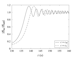
Finally, let us focus our attention on the propagation of the wavetrain front and investigate the effects of the sound speed  $c$ on the amplitude ratio (3.7). Figures 3(a) and 3(b) show the behaviour of the envelope amplitude ratio
  $|{\mathcal{B}}_{m}/{\mathcal{B}}_{m0}|$ versus time
  $t$, for fixed
  $x=2\times 10^{5}~\text{m}$,
  $\unicode[STIX]{x1D714}=2~\text{rad}~\text{s}^{-1}$ and integers
  $m=0,1$, respectively. Similarly, figures 3(c) and 3(d) show the same physical quantity but for larger frequency, i.e.
  $\unicode[STIX]{x1D714}=6~\text{rad}~\text{s}^{-1}$. All figures show a similar phenomenon, i.e. the envelope travels faster when
  $c$ corresponds to the Munk profile
  $c_{M}$. For example, figure 3(a) shows that the envelope peak in the case of
  $c=c_{M}$ arrives
  ${\sim}4~\text{s}$ earlier than the envelope peak for
  $c=c_{0}$ constant. Furthermore, figure 3 also shows that normal modes with smaller
  $m$ index and larger frequency
  $\unicode[STIX]{x1D714}$ reach the steady-state limit
  ${\mathcal{B}}_{m0}$ faster than normal modes with larger vertical eigenvalues and smaller frequencies.

Figure 3. Evolution of the envelope amplitude ratio (3.7) for different sound speed vertical velocities  $c_{M}$ and
  $c_{0}$ and fixed horizontal coordinate
  $x=2\times 10^{5}~\text{m}$: (a)
  $\unicode[STIX]{x1D714}=2~\text{rad}~\text{s}^{-1}$ and
  $m=0$, (b)
  $\unicode[STIX]{x1D714}=2~\text{rad}~\text{s}^{-1}$ and
  $m=1$, (c)
  $\unicode[STIX]{x1D714}=6~\text{rad}~\text{s}^{-1}$ and
  $m=0$, while (d)
  $\unicode[STIX]{x1D714}=6~\text{rad}~\text{s}^{-1}$ and
  $m=1$.
5 Conclusions
We analysed the propagation of HA waves in the presence of a depth-dependent sound speed profile using a perturbation expansion up to the third order, three timing and two slow horizontal length scales.
At the second order, we found a correction for the velocity potential due to the variation of the sound speed in the fluid. We showed that the potential can be significantly affected if the sound speed is not constant throughout the fluid layer, and that the frequency increases or decreases depending on the profile, with effects on the phase speed. This clearly has implications for the dynamic pressure distribution in the fluid domain, a physical quantity of interest for detecting HA waves with hydrophones and underwater equipment.
At the third order, asymptotic analysis for the Schrödinger equation allowed us to describe the behaviour of the envelope front in terms of Fresnel integrals. We compared the results obtained in the case of a Munk profile, valid in deep oceanic waters, with the case of a constant sound speed. The idealised Munk profile is mainly used to simulate deep-water propagation in mid-latitude oceanic waters having depth exceeding 2000 m and has been widely applied in computational ocean acoustics. We found that the envelope travels faster in the case of the Munk profile. This result highlights the importance of including variable sound speed vertical profiles in the design of tsunami early warning systems based on HA waves. Finally, we investigated the envelope propagation for different normal modes and frequencies. Our results show that the evolution reaches a steady state faster when the frequency increases and when the mode number decreases.
Other effects such as variable topography or seabed attenuation are inevitable as one get closer to the nearshore environment. These phenomena complicate the dynamics and should also be investigated to better evaluate the propagation of HA waves for practical applications.
Acknowledgements
The work of S.M. is supported by a Royal Society–CNR International Fellowship. E.R. acknowledges financial support from EPSRC (First Grant EP/R015899/1).


