


1. Introduction
Internal waves (IWs), propagating through density-stratified media in a rotating frame of reference, are common features in the ocean which affect circulation and are believed to close the ocean energy budget by dissipating approximately 25 % to 30 % of tidal energy (Garrett & Munk Reference Garrett and Munk1979; Munk & Wunsch Reference Munk and Wunsch1998; Egbert & Ray Reference Egbert and Ray2000). Consequently, IW generation and propagation have received considerable focus over the past several decades (Rattray Reference Rattray1960; Bell Reference Bell1975; Baines Reference Baines1982). IWs, particularly internal tides, are often generated through the vertical acceleration of tidal currents over a sloping topography (i.e. ridges or continental shelf breaks) causing vertical fluctuations of isopycnals (Rattray Reference Rattray1960; Baines Reference Baines1974; Bell Reference Bell1975; Holloway & Merrifield Reference Holloway and Merrifield1999; Merrifield & Holloway Reference Merrifield and Holloway2002; Klymak et al. Reference Klymak, Moum, Nash, Kunze, Girton, Carter, Lee, Sanford and Gregg2006). To quantify IW generation due to flow–topography interactions, the conversion rate ( $C$) of barotropic (BT) to baroclinic (BC) energy is often used (Merrifield, Holloway & Johnston Reference Merrifield, Holloway and Johnston2001; Venayagamoorthy & Fringer Reference Venayagamoorthy and Fringer2005; Lamb Reference Lamb2007; Moum et al. Reference Moum, Klymak, Nash, Perlin and Smyth2007; Kang & Fringer Reference Kang and Fringer2010, Reference Kang and Fringer2012; Lien et al. Reference Lien, Henyey, Ma and Yang2014; Palmer et al. Reference Palmer, Stephenson, Inall, Balfour, Düsterhus and Green2015). The value of
  $C$ is commonly estimated using a time-invariant background density profile, and then averaged over a tidal cycle to estimate topographic conversion (Kang & Fringer Reference Kang and Fringer2012; Müller Reference Müller2013). These methods provide reliable estimates of
  $C$ due to flow over topography. However, they are generally limited to linear waves and do not provide insight into the evolution and dynamics of BT to BC energy conversion through time, or due to other processes such as vertical fluid displacements caused by tides and other IWs. Here, we introduce a dynamic decomposition of the BC energy budget that accurately accounts for BT tidal heaving (BTH) using a time-varying background density, allows for investigation of the conversion dynamics through time or over depth and is not limited to linear IWs.
The value of  $C$ depends on the density (pressure) perturbation, the BT velocity and the topographic slope. In the absence of a sloping ocean bottom, tides lead to vertical displacement of the water surface and constant density surfaces (isopycnals) with associated vertical velocities. The phase difference between the displacement of isopycnals and vertical velocity leads to BT–BC conversion that sums to zero over a tidal cycle. Thus, in the absence of a sloping topography, a stratified fluid heaves up and down without a net conversion of energy to other modes. However, IWs can interact with BTH, which results in energy conversion that is not due to flow–topography interaction. In addition to BTH, the presence of remotely generated IWs in coastal regions can affect IW generation when tides and remotely generated waves are phase locked (Kelly & Nash Reference Kelly and Nash2010; Zilberman et al. Reference Zilberman, Merrifield, Carter, Luther, Levine and Boyd2011; Nash et al. Reference Nash, Shroyer, Kelly, Inall, Duda, Levine, Jones and Musgrave2012; Pickering et al. Reference Pickering, Alford, Nash, Rainville, Buijsman, Ko and Lim2015). Finally, IWs can interact with each other scattering energy back to BT or into other BC modes. We refer collectively to these additional sources of conversion (tide–wave,
  $IW\times BTH$, and wave–wave,
  $IW\times IW$, interactions) as ‘residual conversion’ as they are extraneous to, but may affect estimates of, topographic conversion. Accurate accounting of these types of conversion also allows for investigations of these interactions.
In order to estimate the topographic conversion, it is important to recognize and partition the density (pressure) perturbations effectively to isolate the conversion induced by local flow–topography interaction. Llewellyn, Stefan & Young (Reference Llewellyn, Stefan and Young2002) discarded the nonlinear advection and dissipation terms in the Boussinesq momentum equations which resulted in  $C=p'|_{z=-H}\boldsymbol {U}\boldsymbol {\cdot }\boldsymbol {\nabla }H$ (hereinafter the LSY method) where
  $p'$,
$p'$,  $\boldsymbol{U}$ and H are pressure perturbation, BT horizontal velocity and ocean bottom. This method has been widely used in the literature (Kurapov et al. Reference Kurapov, Egbert, Allen, Miller, Erofeeva and Kosro2003; Gerkema, Lam & Maas Reference Gerkema, Lam and Maas2004; Carter et al. Reference Carter, Merrifield, Becker, Katsumata, Gregg, Luther, Levine, Boyd and Firing2008; Kelly & Nash Reference Kelly and Nash2010; Kelly, Nash & Kunze Reference Kelly, Nash and Kunze2010; Pickering et al. Reference Pickering, Alford, Nash, Rainville, Buijsman, Ko and Lim2015). The LSY method partially removes residual conversion through the topographic slope term. Kang & Fringer (Reference Kang and Fringer2012) included nonlinear advection and dissipation terms to arrive at
  $C=\rho 'gW$ (where
  $\rho'$, g and W are density perturbation, gravitational acceleration, and BT vertical velocity), and removed residual conversion through tidal averaging. To filter the residual conversion, others (Lu, Wright & Brickman Reference Lu, Wright and Brickman2001; Kunze et al. Reference Kunze, Rosenfeld, Carter and Gregg2002; Zilberman et al. Reference Zilberman, Merrifield, Carter, Luther, Levine and Boyd2011) used an approximation for the linear IW potential energy and removed the BT vertical displacement caused by surface tides over a sloping topography as approximated by Baines (Reference Baines1982). Kelly et al. (Reference Kelly, Nash and Kunze2010) developed a method based on modal decomposition to account for BTH and IW interactions. Pollmann et al. (Reference Pollmann, Nycander, Eden and Olbers2019) further proposed a semi-analytical method which gives a positive definite conversion field for linear IWs over a subcritical bathymetry through spatial smoothing. These methods, however, are generally based on a constant (time-invariant) background density (CBD), disregard nonlinear advection terms (in some cases, diffusion–dissipation terms are also neglected, except see Kang & Fringer Reference Kang and Fringer2012), which limits the scope of these analyses to linear IWs, and are predicated on tidal averaging to remove residual conversion. Tidal averaging, while effective, prevents the investigation of the dynamics of IW generation and BT–BC conversion at short time scales (e.g. over a tidal cycle).
Here, we directly account for BTH using a time-varying background density (TVBD). The concept of TVBD has been previously applied to study mixing (MacCready & Giddings Reference MacCready and Giddings2016; Dossmann et al. Reference Dossmann, Pollet, Odier and Dauxois2017), but has not been used to study IW generation. We build on the formulation offered by Kang & Fringer (Reference Kang and Fringer2012)  $C=\rho ' g W$ (hereinafter the KF method) by decomposing the Reynolds-averaged Navier–Stokes equations while retaining the nonlinear advection and dissipation terms. This implementation results in a new term in the BC energy budget that represents
  $IW\times BTH$ conversion, and conversion associated with IW reflection depending on how the TVBD is formulated. We show that this term accurately accounts for
  $IW\times BTH$ conversion using a background density that changes due to tides. We also show that
  $\rho _b$ must be modified beyond accounting for BTH in order to isolate the effects of
  $IW\times IW$ conversion using an idealized three-dimensional (3-D) set-up. We develop the theoretical framework in § 2. In § 3, we outline the numerical model set-up. We discuss the application of the theoretical framework and interpret the results in § 4, and conclude the paper with a summary in § 5.
2. Theoretical framework
Under the Boussinesq approximation, conservation of mass and the Reynolds-averaged Navier–Stokes equations are
 \begin{gather} \boldsymbol{\nabla}\boldsymbol{\cdot}\boldsymbol{u}=0, \end{gather}
 \begin{gather}\frac{\partial u}{\partial t}+(\boldsymbol{u}\boldsymbol{\cdot}\boldsymbol{\nabla}){u}-f v={-}\frac{1}{\rho_0} \frac{\partial P}{\partial x}+ \boldsymbol{\nabla}\boldsymbol{\cdot}(\nu_h \boldsymbol{\nabla}_h u)+\frac{\partial}{\partial z}\left(\nu_v \frac{\partial u}{\partial z}\right), \end{gather}
 \begin{gather}\frac{\partial v}{\partial t}+(\boldsymbol{u}\boldsymbol{\cdot}\boldsymbol{\nabla}){v}+f u={-}\frac{1}{\rho_0} \frac{\partial P}{\partial y}+ \boldsymbol{\nabla}\boldsymbol{\cdot}(\nu_h \boldsymbol{\nabla}_h v)+\frac{\partial}{\partial z}\left(\nu_v \frac{\partial v}{\partial z}\right), \end{gather}
 \begin{gather}\frac{\partial w}{\partial t}+(\boldsymbol{u}\boldsymbol{\cdot}\boldsymbol{\nabla}){w}={-}\frac{1}{\rho_0} \frac{\partial P}{\partial z}+ \boldsymbol{\nabla}\boldsymbol{\cdot}(\nu_h \boldsymbol{\nabla}_h w)+\frac{\partial}{\partial z}\left(\nu_v \frac{\partial w}{\partial z}\right)- \frac{\rho}{\rho_0}g, \end{gather}
where  $u,v,w,P,f$,
  $\nu _h$ and
  $\nu _v$ are velocity in x, y and z directions, pressure, the Coriolis frequency, and the horizontal and vertical eddy viscosities, respectively. Pressure and density are partitioned into reference, background and perturbation components, and velocities are decomposed into BT and BC components
 \begin{gather} \rho=\rho_0+\rho_b+\rho', \end{gather}
 \begin{gather}P=P_0+P_b+P'=g \int_{z}^{\eta} \left( \rho_0+\rho_b(z')+\rho'(z')\right) {\rm d}z', \end{gather}
 \begin{gather}\boldsymbol{U_h}=\frac{1}{H}\int_{{-}d}^{\eta} \boldsymbol{u_h}= \frac{1}{H} \overline{\boldsymbol{u_h}}\,{\rm d}, \end{gather}
 \begin{gather}\boldsymbol{\nabla}\boldsymbol{\cdot}\boldsymbol{U}=0, \end{gather}
 \begin{gather}\boldsymbol{\nabla}\boldsymbol{\cdot}\boldsymbol{u'}=0, \end{gather}
where the  $\boldsymbol {h}$ subscript denotes the horizontal (
 $x,y$ and
  $u,v$),
  $H=\eta +d$ is the water column depth (
 $\eta$ and
  $-d$ are sea surface height and ocean bottom, respectively), the bar operator provides the depth-integrated value of a parameter (
 $\bar {\psi }=\int _{-d}^{\eta }\psi \,{\rm d} z$) and capital letter velocities (
 $U$,
$U$, $V$) are the BT components, while the prime velocities (
 $u'$,
$u'$, $v'$) are the BC constituents. The BT and BC vertical velocities can be found using the continuity equation
  $W=-\boldsymbol {\nabla }_h\boldsymbol {\cdot }(\boldsymbol {U}_h (d+z))$ and
  $w'=w-W$, respectively.
By using the momentum equations and applying boundary conditions (full derivation is provided in Kang (Reference Kang2010) and summarized in Appendix A), we get the depth-integrated BC kinetic energy ( $E'_K$) budget
 \begin{align} \frac{\partial \overline{E'_K}}{\partial t}+\boldsymbol{\nabla_h} \boldsymbol{\cdot}(\overline{\boldsymbol{u_h}E'_K})+\boldsymbol{\nabla_h} \boldsymbol{\cdot}(\overline{\boldsymbol{u'_h}E_{K_{BT-BC}}}) &={-}\boldsymbol{\nabla_h} \boldsymbol{\cdot}(\overline{\boldsymbol{u_h'}P'})-\overline{\rho'gw'}+A_h \nonumber\\ &\quad +\overline{\boldsymbol{\nabla_h}\boldsymbol{\cdot}(\nu_H\boldsymbol{\nabla_h}E'_K)} -D'-\overline{\epsilon_K}. \end{align}
where  $A_h, D', \epsilon_K$ are unclosed, drag and dissipation terms respectively.
For an incompressible density-stratified fluid, the available potential energy ( $E_A$) is equal to the difference between the potential energy of the perturbed water column (
 $E_P$) and the minimum energy attainable thorough adiabatic motion (
 $E_B$) (Lorenz Reference Lorenz1955; Winters et al. Reference Winters, Lombard, Riley and D'Asaro1995). The concept of
  $E_A$ has been widely used to study energy budgets in both deep and shallow water systems (Venayagamoorthy & Fringer Reference Venayagamoorthy and Fringer2005; Klymak et al. Reference Klymak, Moum, Nash, Kunze, Girton, Carter, Lee, Sanford and Gregg2006; Scotti, Beardsley & Butman Reference Scotti, Beardsley and Butman2006; Kang & Fringer Reference Kang and Fringer2010, Reference Kang and Fringer2012). For any arbitrary density stratification,
  $E_A$ can be found from (Kang & Fringer Reference Kang and Fringer2010, Reference Kang and Fringer2012)
 \begin{equation} E_A=E_P-E_B=g\int_{z-\delta}^{z} \left(\rho(z)-\rho_b(z')-\rho_0 \right) {\rm d}{z'}, \end{equation}
where  $\delta$ is the BT and BC vertical displacement of isopycnals. For linear IWs in linear density-stratified media,
  $E_A$ can further be approximated as (Gill Reference Gill1982; Scotti et al. Reference Scotti, Beardsley and Butman2006; Lamb Reference Lamb2007)
 \begin{equation} E_A=\frac{\rho_0}{2}N^2\delta^2=\frac{g^2 \rho'^2}{2\rho_0 N^2}, \end{equation}
where  $N^2=-({g}/{\rho _0})({\partial \rho }/{\partial z})$ is the squared Brunt–Väisälä frequency. The
  $E_A$ inside a system can be dissipated, advected or converted to kinetic energy (disregarding the spatio-temporal background density variation
  ${\partial \rho _b}/{\partial x}, {\partial \rho _b}/{\partial y}, {\partial \rho _b}/{\partial t}\approx 0$)
 \begin{equation} \overline{\frac{\partial E_A}{\partial t}}+\overline{\boldsymbol{u}\boldsymbol{\cdot}\boldsymbol{\nabla}E_A}=\overline{g w \rho'(z)}+\overline{\epsilon_A}. \end{equation}
where  $\epsilon_A$ is the diffusion of potential energy.
By adding (2.10) and (2.13) and tidally averaging, we get
 \begin{align} & \boldsymbol{\nabla_h}\boldsymbol{\cdot}\left\langle \overline{\boldsymbol{u}\boldsymbol{\cdot}\boldsymbol{\nabla}E_A}+ \overline{\boldsymbol{u_h}E'_k}+\overline{\boldsymbol{u'_h}EK_{BT-BC}}+ \overline{\boldsymbol{u_h'}P'}-\overline{\nu_H\boldsymbol{\nabla_h}E'_K}\right\rangle= \langle\overline{\rho'gw}-\overline{\rho'gw'}\rangle \nonumber\\ &\quad +\langle A_h\rangle-\langle D'\rangle\langle\overline{\epsilon_A-\epsilon_K}\rangle, \end{align}
where the angle bracket operator provides the tidally averaged value of a parameter over a period of T ( $\langle \psi \rangle =({1}/{T})\int _{0}^{T} \psi \,{\rm d} t$). The energy conversion rate from BT to BC modes can be found by the summation of
  $\rho 'gw$ and
  $-\rho 'gw'$ (Kang & Fringer Reference Kang and Fringer2012). In such a formulation,
  $C$ consists of both topographic and residual conversion. BTH of isopycnals alone (without the presence of a sloping bottom) does not generate IWs nor convert energy from BT to BC; yet, vertical acceleration over a sloping topography causes a phase lag between the density perturbation and the vertical velocity,
  $\phi _{\rho ',W}$ (where
  $\phi _{a,b}$ denotes the phase difference between a and b). The conversion that occurs due to the phase lag between the density perturbation and the vertical velocity can be understood by considering two idealized sinusoidal functions assigned to
  $\rho '$ and
  $W$ with period, amplitude and initial phase of
  $\omega$,
  $a$ and
  $b$
$b$
 \begin{equation} \langle C \rangle=\langle \rho'gW \rangle=g\left\langle a_i\sin(\omega t+b_i) a_j\sin(\omega t+b_j)\right\rangle=g\frac{a_ia_j}{2}\cos(\phi_{b_i,b_j}) \end{equation}
leading to positive (negative) conversion rates for phase differences  $<90^\circ$ (
 $>90^\circ$) (Zilberman et al. Reference Zilberman, Becker, Merrifield and Carter2009).
To better understand how BTH contributes to conversion, we consider a system governed by tidal flows with a flat bathymetry in which isopycnals heave up (down) during flood (ebb) tides and  $\phi _{W, \rho '} = 90^\circ$. Figure 1 depicts the characteristics of such a system where there are non-zero density perturbations (red curve in figure 1c) and BT vertical velocities (figure 1d) through time. The density perturbations captured by CBD methods is completely induced by BTH (compare panels (b) and (c) in figure 1). Due to the failure of BTH filtering in
  $\rho _B$ a non-zero
  $C$ emerges with a zero tidally averaged value (red curve in figure 1f) which is fully BT. By applying a proper time-varying
  $\rho _b$, the BT displacement of the background density is removed (blue curve in figure 1c); therefore, the residual conversion is eliminated (blue curve in figure 1f).

Figure 1. Times series of tidal flow over flat bottom showing (a) tidal height, (b) background density, (c) density perturbation, (d) BT vertical velocity at mid-depth, (e) BT conversion rate where  $\varDelta \rho _b$ is difference between TVBD and CBD background density and (f) BT–BC conversion rate.
In CBD methods (e.g. both LSY and KF),  $\rho _b$ is only a function of
  $z$; while in TVBD,
  $\rho _b$ is a function of
  $z$ and
  $t$. The temporal dependency of
  $\rho _b$ creates a new cross-term in the
  $E_A$ budget which can remove arbitrary vertical displacements (a similar methodology was used by Lu et al. Reference Lu, Wright and Brickman2001; Kunze et al. Reference Kunze, Rosenfeld, Carter and Gregg2002; Zilberman et al. Reference Zilberman, Merrifield, Carter, Luther, Levine and Boyd2011). By removing the BT displacement at any depth we can remove the effects of BTH. To do so, we assume that BT tidal height varies linearly over the water column as
  $\gamma (x,y,z,t)=\eta (1-{z}/{H})$.
The contribution of nonlinear advection terms in the  $E_A$ budget in the formation of
  $\rho ' g W$ is acknowledged by Kang & Fringer (Reference Kang and Fringer2012). Accounting for nonlinear advection terms results in an additional term in the
  $E_A$ budget (see Appendix A for full derivation)
 \begin{equation} \overline{\frac{\partial E_A}{\partial t}}+\overline{\boldsymbol{u}\boldsymbol{\cdot}\boldsymbol{\nabla}E'_K} = \overline{\rho'g w }-\overline{g \int_{z-\delta}^{z}\frac{\partial \rho_b(z',t)}{\partial t} {\rm d} z'}+ \overline{\epsilon_A}. \end{equation}
 The total energy budget (kinetic+potential), where  $\langle \overline {\rho ' gW-g \int _{z-\delta }^{z}({\partial \rho _b(z',t)}/{\partial t} \,{\rm d} z'})\rangle$ is the modified conversion, then becomes
 \begin{align} & \boldsymbol{\nabla_h}\boldsymbol{\cdot}\left\langle \overline{\boldsymbol{u}\boldsymbol{\cdot}\boldsymbol{\nabla}E_A}+\overline{\boldsymbol{u_h}E'_k}+ \overline{\boldsymbol{u'_h}EK_{BT-BC}}+\overline{\boldsymbol{u_h'}P'}- \overline{\nu_H\boldsymbol{\nabla_h}E'_K}\right\rangle \nonumber\\ &\quad =\left\langle\overline{\rho'gW-g \int_{z-\delta}^{z} \frac{\partial \rho_b(z',t)}{\partial t} {\rm d} z'}\right\rangle +\langle A_h\rangle-\langle D'\rangle+\langle\overline{\epsilon_A-\epsilon_K}\rangle. \end{align}
 This formulation can be considered a modified version of Kang & Fringer (Reference Kang and Fringer2012). The contribution of the non-hydrostatic pressure ( $-\overline {({\partial q}/{\partial z})W}$ where
  $q$ is the non-hydrostatic pressure constituent) can be added directly to this formulation (Kang & Fringer Reference Kang and Fringer2012). The new term in (2.17) can isolate the conversion due to the interaction of IWs and BTH (
 $IW \times BTH$) and even between IWs (
 $IW \times IW$) if the background density is formulated accordingly.
3. Numerical set-up
To test the TVBD method and the resulting effects on  $C$, we simulated IW generation using SUNTANS (Stanford unstructured non-hydrostatic terrain following averaged Navier–Stokes simulator). SUNTANS is a finite volume model that solves 3-D non-hydrostatic, nonlinear Navier–Stokes equations on unstructured–triangular horizontal grids with
  $z$-level vertical layers (Fringer, Gerritsen & Street Reference Fringer, Gerritsen and Street2006). SUNTANS has been widely used to study non-hydrostatic, nonlinear phenomena such as IWs and circulation in shallow coastal systems and estuaries (Jachec et al. Reference Jachec, Fringer, Street and Gerritsen2007; Zhang, Fringer & Ramp Reference Zhang, Fringer and Ramp2011; Kang & Fringer Reference Kang and Fringer2012; Nelko, Saha & Chua Reference Nelko, Saha and Chua2014; Xu & Chua Reference Xu and Chua2016). We begin our analysis with two idealized 2-D cases with high spatio-temporal resolution to highlight the TVBD method and compare it to other common methods. To validate the formulation in a more realistic set-up, we compared the results for an idealized 3-D ridge. The bathymetry for the 2-D and the 3-D set-ups can be seen in figures 2 and 3, respectively.

Figure 2. Vertical velocity at time  ${t}/{T}=0.4$ for (a) shallow (case 1) and (b) deep (case 2) scenarios. The generation site over the topographic feature (green circle) and a site of IW reflection from the ocean surface (purple circle) are shown.

Figure 3. Ideal ridge bathymetry map (a, case 3) and its transects at (b)  $X= 300$ km and (c)
  $Y= 50$ km.
For all cases, we applied a constant background horizontal turbulent viscosity of 1 m $^{2}$ s
 $^{-1}$ and employed a Mellor–Yamada 2.5 (MY 2.5) turbulence closure scheme for the vertical turbulent viscosity (Mellor & Yamada Reference Mellor and Yamada1982). The horizontal viscosity was set to the minimum value needed to remove numerical oscillations between grid points (10 m resolution). The shortest wavelengths possible in the domain are
  $O$(60 m), so this did not affect IW generation. We also ran cases with
  $\nu _h = 0.1$, 0.01 and 0.001 m
 $^2$ s
 $^{-1}$ and constant
  $\nu _v = 0.001$ and 0.0001 m
 $^2$ s
 $^{-1}$. Results of all cases were consistent, we therefore only report cases with
  $\nu_h = 1$ m
 $^{2}$ s
 $^{-1}$ and the MY 2.5 closure scheme.
To analyse the effect of depth (shallow vs deep) on  $C$, we used idealized functions for density stratification (figure 4) and bathymetry
 \begin{equation} d=H_0 - 0.5(H_0-h_0)\left(1+\tanh\left(\frac{x-X_{mid}}{L_s}\right)\right), \end{equation}
where  $h_0$ and
  $H_0$ are constants (minimum and maximum depths in the domain),
  $d$ is the depth at any specific point,
  $X_{mid}$ and
  $L_s$ are bathymetric shape constants.

Figure 4. Background density and Brunt–Väisälä frequency at the beginning of the last 3 tidal cycles for (a) shallow (case 1) and (b) deep (cases 2 and 3) cases.
For all cases,  $M_2$ tidal currents (
 $u=U_0 \sin (\omega t)$) were applied at the ocean-side boundary barotropically and the shore-side boundary was closed. To avoid IW reflection from offshore and onshore boundaries,
  $u'$ was relaxed using a sponge layer that extended 20 km into the domain at each side. The Coriolis frequency was set to
  $0.8 \times 10^{-4}$ s
 $^{-1}$ representing
  ${\sim }33 ^{\circ }$N latitude. We chose this mid-latitude as it represents a value close to the region (central California) that motivated this study. However, our results were again consistent regardless of the value of
  $f$ used based on additional simulations.
We examined three case scenarios (shallow 2-D shelf, deep 2-D shelf, 3-D ridge) with different physical inputs (tidal current velocity, bathymetry, eddy viscosity) and environmental parameters (domain size and spatio-temporal resolution) as summarized in table 3 in Appendix A. The models were run for 15 tidal cycles and all analyses were performed on the last 3 tidal cycles. Model set-up files and analysis scripts are available on GitHub at https://github.com/somidvar/suntans/tree/master/TVBDPaperSourceCode.
4. Results and discussion
In this section, we compare the results of CBD methods (LSY, KF) with the TVBD method and show how TVBD provides an improvement by directly allocating topographic and residual conversion. The steepness number ( $\beta _1$) and tidal excursion (
 $\beta _2$) are informative dimensionless numbers characterizing the reflectivity and period of IWs
 \begin{gather} \beta_1=\frac{\tan(\theta_{B})}{\tan(\theta_{IW})}= \sqrt{\frac{\left(\dfrac{\partial d}{\partial x}\right)^2+\left(\dfrac{\partial d}{\partial y}\right)^2}{\dfrac{\omega^2-f^2}{N^2-\omega^2}}}, \end{gather}
 \begin{gather}\beta_2=\frac{U_0k_b}{\omega}, \end{gather}
where  $\theta$,
  $U_0$ and
  $k_b^{-1}$ are the angle (subscripts
  $_B$ and
  $_{IW}$ denote ocean bottom and IW) with the horizontal, maximum BT tidal current velocity and topographic length scale. For IW studies,
  $k_b$ is estimated as
  ${\theta _{B}}/{(H-d)}$ (Garrett & Kunze Reference Garrett and Kunze2007; Kang & Fringer Reference Kang and Fringer2012). In a system with supercritical bathymetry (
 $\beta _1>1$), the majority of generated IWs propagate offshore while for a subcritical bathymetry (
 $\beta _1<1$), the IWs also move toward the shore. Tidal excursion,
  $\beta _2$, less than one suggests that the IW frequency is similar to the forcing frequency; while
  $\beta _2>1$ gives lee waves (Kang & Fringer Reference Kang and Fringer2012). For this study, all the cases have super-critical topography (
 $\beta _1>1$) and respond mainly at the perturbation frequency (
 $\beta _2<1$). To insure adequate conversion for our analyses, we set our cases with
  $1<\beta _1\leq 8$ (Kang & Fringer Reference Kang and Fringer2012). Therefore, we expect to see generated IWs propagating offshore as IW beams. The generated IWs can clearly be seen as elevation and depression rays as they bounce from ocean bottom and surface (figure 2).
4.1. Residual conversion in time series
The main difference between TVBD and CBD methods is the direct accounting for  $IW \times BTH$ by TVBD. The conversion rate is the product of
  $W$ and
  $\rho '$ in which the density perturbation is induced by density changes due to BTH, vertical acceleration over a sloping bathymetry and BC oscillations. BTH results in a residual positive–negative conversion with a magnitude of
  $(\rho _{b_{TVBD}}-\rho _{b_{CBD}})g W$, and is responsible for the observed difference between CBD and TVBD results. Figure 5, which follows the same layout as figure 1, illustrates the difference between the two methods at the generation site (panels (d,e) and (i,j) which corresponds to 2 and
  $12 \times 10^{-4}$ W m
 $^{-2}$ for shallow and deep cases, respectively). Although the LSY method removes the background pressure
  $P_b$, this issue persists as it only removes the time-averaged background pressure
  $P_b$ and not BTH. The presence of residual positive–negative conversion in the
  $C$ time series shown in figures 5(e) and 5(j) supports this assertion.

Figure 5. Time series of parameters involved in BT–BC conversion shown at generation sites (green circles in figure 2; left and right panels are for cases 1 and 2, respectively). (a,f) Background density, (b,g) perturbation density, (c,h) BT vertical velocity, (d,i) BT conversion rate where  $\varDelta \rho _b$ is the difference between TVBD and CBD background density and (e,j) BT–BC conversion rate as in figure 1.
4.2. Non-zero residual conversion over flat bottom
At reflection points, where the IWs bounce from the ocean surface and bottom, there is no active IW generation. However, residual  $C$ occurs due to disturbances caused by BTH and other IWs, which is accounted for in the new interaction term of the TVBD formulation (
 $IW \times BTH$). Similar patterns have been reported by incoherent remotely generated IWs, which are phase locked to the surface tides by Kelly & Nash (Reference Kelly and Nash2010), Zilberman et al. (Reference Zilberman, Merrifield, Carter, Luther, Levine and Boyd2011) and Pickering et al. (Reference Pickering, Alford, Nash, Rainville, Buijsman, Ko and Lim2015). Based on Zilberman et al. (Reference Zilberman, Becker, Merrifield and Carter2009), the energy conversion is due to
  $\cos (\phi _{\rho ',W})$, which can be affected by the presence of IWs. As shown in figure 6, the reflected IWs from the ocean surface and bottom possess
  $w'$ (BC perturbations shown in (c,h)) which is not in phase with BT vertical movement; therefore, altering the phase of
  $\rho '$ slightly (b,g). Conversion due to IW reflection is retained in the CBD conversion calculation as it creates residual conversion (positive or negative) away from the generation sites. Figures 7(a) and 7(c), which demonstrate the time-averaged conversion rate in the model, clearly shows the alternating shading pattern of the CBD method. In contrast, the TVBD method removes the effects of IW reflection on
  $C$ through the
  $IW \times BTH$ term (figure 6d). This issue is masked in the LSY method as it depends on the topographic slope, which is zero away from the slope in this study. However, disregarding the topographic slope in the LSY formulation (
 $P'|_{z=-H} \boldsymbol {U}\boldsymbol{\cdot} \boldsymbol {I}$ where
  $I=(1,1,1)$ is the unity vector), we observe an oscillating pattern similar to the KF method as it retains non-zero residual conversion over the flat part of the domain. Figures 8(b) and 8(d), which provide the time-averaged depth-integrated conversion rate, show such an issue for the LSY method (panels (a) and (c) demonstrate the results of KF and TVBD methods). In real scenarios, the ocean bottom is not completely flat near the continental shelf break or ridges so residual conversion may be retained in the topographic conversion term leading to a potential overestimate/underestimate of total topographic conversion.

Figure 6. Time series of parameters involved in BT–BC conversion shown at reflection sites (purple circles in figure 2; left and right panels are for cases 1 and 2, respectively). (a,f) Background density, (b,g) perturbation density, (c,h) BT vertical velocity, (d,i) BT conversion rate where  $\varDelta \rho _b$ is the difference between TVBD and CBD background density and (e,j) BT–BC conversion rate as in figure 1.

Figure 7. Time-averaged conversion rate  $\langle C \rangle$ for case 1 (a,b) and case 2 (c,d) for (a,c) the KF method and (b,d) the TVBD method.
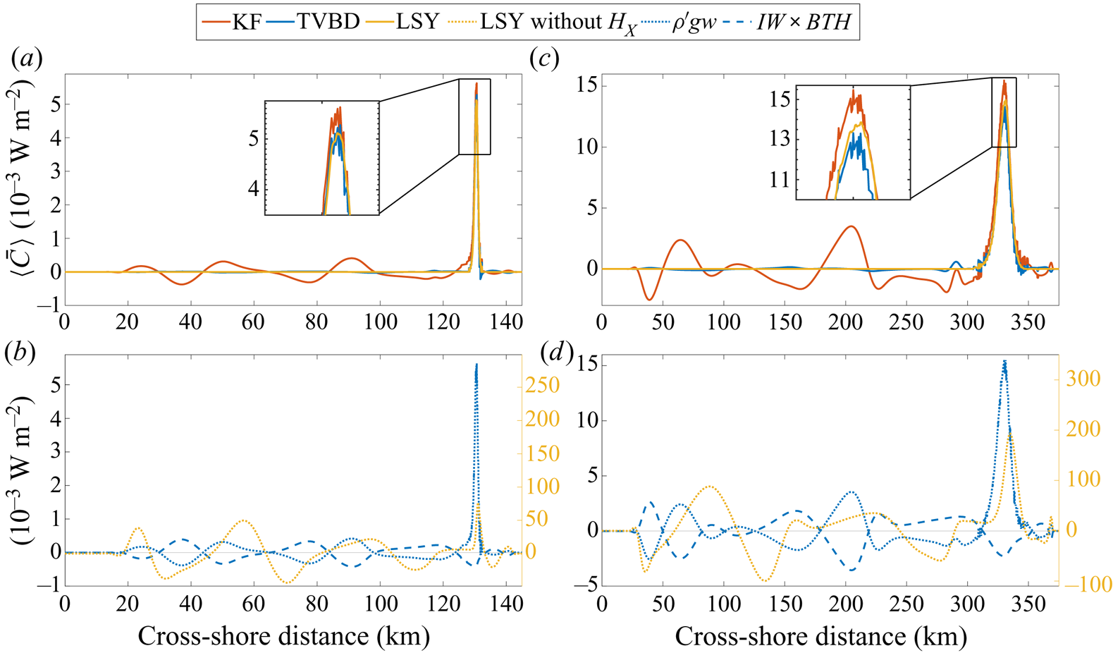
Figure 8. Time-averaged depth-integrated conversion rate ( $\langle \bar {C} \rangle$) for KF, LSY and TVBD methods for shallow (a,b) and deep (c,d) cases. (a,c) A comparison between the three methods over the cross-shore model domain. (b,d) Detail of the two terms of the TVBD method and the LSY method results without the bathymetry gradient
  $H_x$.
To better understand the role of  $IW \times BTH$ we can decompose the tidal average using Leibniz's integral rule
  $\langle IW \times BTH \rangle =-g\int _{0}^{T}\int _{z-\delta }^{z} ({\partial \rho _b(z',t)}/{\partial t})\,{\rm d} z' {\rm d} t$
 $=g \int _{0}^{T}({\partial \delta }/{\partial t})\rho _b(z-\delta ,t)\,{\rm d} t-g \int _{0}^{T}({\partial }/{\partial t})\int _{z-\delta }^{z} \rho _b(z',t)\,{\rm d} z'\,{\rm d} t$ where the first term on the right-hand side is the net conversion over a tidal cycle, and the second term is zero. In the KF method,
  ${\partial \delta }/{\partial t} = w$; however, in the TVBD method,
  ${\partial \delta }/{\partial t} = w'$ as
  $W$ is removed from
  $w$ (figure 6c,g). With
  $\gamma (x,y,z,t)=\eta (1-{z}/{H})$ defined as the BT vertical displacement in a system with flat bathymetry, we can infer that
  $\rho _b(z,t)$ and
  $\rho _b(z-\delta ,t)$ are temporally in phase. For gravitational waves (away from their generation site),
  $\langle \overline {\rho ' g W}\rangle$ and
  $\langle \overline {IW \times BTH}\rangle$ are at complementary angles; therefore, their cosines cancel each other (Cushman-Roisin & Beckers Reference Cushman-Roisin and Beckers2013)
 \begin{equation} \phi_{\rho',w'}+\phi_{\rho_b,W}={\rm \pi} , \end{equation}
and  $IW \times BTH$ cancels any conversion induced by
  $\rho ' g W$ over flat bathymetry.
The overall differences in the estimation of  $C$ at generation points by the LSY and KF methods are minor (less than 5 % and 10 %, respectively) due to the interaction of BTH with the IWs (figure 8; similar to the residuals in § 4b). This overestimation, however, is compensated by negative
  $C$ away from the slope as the spatial integrals of
  $C$ for the LSY, KF and TVBD methods are similar.
In a similar context, Kelly et al. (Reference Kelly, Nash and Kunze2010) decomposed and removed shoaling IWs (waves become steeper and more nonlinear as they approach the shore) which resembles the role of BTH in this study. This requires discerning the phasing of other phenomena like shoaling IW or BTH. Determining the phase, however, is not trivial since the phase changes as a wave propagates in the system. Phase variation is obvious as the magnitudes of  $W$ and
  $\rho '$ do not vary significantly over the flat bottom part of the domain; yet, there is a meaningful conversion gradient due to
  $\phi _{\rho ', W}$ (figure 8a,c). Also, the modal decomposition utilizes linear superimposition of unwanted (shoaling) and wanted (local) phenomena which may not hold for nonlinear cases.
4.3. Extension to 3-D case
To test the performance of the TVBD method and its extension to a more realistic set-up, we compared the CBD and TVBD results for an idealized ridge case. As shown in figure 9, there is a good agreement between the CBD and TVBD patterns. In the 3-D case, IW reflection and the residual conversion are obvious in the KF method which are removed through the  $IW \times BTH$ term (figure 9b,f). The spatial integral of
  $C$ over the whole domain of the 3-D ridge is equal to 66.5 and 63.5 MW for the KF and TVBD methods, respectively. The TVBD does not remove all residual
  $C$ in the 3-D case especially at the flanks of the ridge due to
  $IW \times IW$ interactions, yet there is still significant improvement in estimates of
  $C$, especially through time as tidal averaging is not needed. We believe that incorporation of IW displacements in the definition of
  $\rho _b$ would remove these regions of residual conversion as well.

Figure 9. (a,b) Show the time-averaged conversion rate ( $\langle C \rangle$) using KF and TVBD at the transect
  $Y=50$ km. The time-averaged depth-integrated conversion rate (
 $\langle \bar {C} \rangle$) at the transect
  $Y=50$ km for both methods can be seen in (c); while the components of TVBD are shown in panel (d). The time-averaged depth-integrated conversion rate for the whole domain can be seen in panels (e) and (f) using KF and TVBD, respectively. Bathymetry contours are spaced at
  $-$300,
  $-$500,
  $-$1000,
  $-$2000 and
  $-$2900 m in (e,f).
5. Conclusion
In this study, we compared BT to BC energy conversion over sloping bottoms using a new time-variant background density method to commonly used methods (LSY and KF) utilizing CBD. Table 1 highlights the (dis)advantages of each method as well as the numerical results for one of the case scenarios. Our method allows for analysis of conversion through time and over depth, while also removing residual conversion. TVBD provides greater analytical detail because the method is derived directly from the governing equations. However, our analysis confirms the effectiveness of other methods that work for field data where the resolution is limited in time and space for depth-integrated, time-averaged values (similar values of  $\int _{0}^{X} \langle \bar {C} \rangle \,{\rm d} x$ in table 1).
Table 1. Comparison of methods for estimating BT–BC conversion;  $C_{max}$ and
  $C_{min}$ are the maximum and minimum conversion during the whole run time at
  $x,z$ of 331 km, 613 m where the maximum conversion occurs,
  $[\langle \bar {{C}} \rangle ]_{x=max}$ and
  $[\langle \bar {{C}} \rangle ]_{x=min}$ are the maximum and minimum values across shore during the entire run time.

A portion of BT tidal energy is converted to the BC energy over sloping topography due to the phase difference between the BT vertical velocity  $W$ and the density perturbation
  $\rho '$. The density perturbation is the result of BTH, local acceleration over the sloping bottom and BC oscillations. CBD methods attempt to remove the BTH effects by averaging over tidal cycles. However, these methods suffer from the presence of residual values in
  $C$ time series although the net tidally averaged
  $C$ is zero (
 $C_{min}$ values in table 1 are more negative in KF than TVBD). The need to tidally average limits the utility of CBD methods to time scales longer than a tidal cycle. The TVBD method remedies this issue through an additional term representing the interaction between BTH and IWs. The TVBD method also provides an improvement over modal decomposition methods (Kelly et al. Reference Kelly, Nash and Kunze2010) because wave–tide interactions are removed directly through the
  $IW \times BTH$ term;
  $IW \times BTH$ emerges in the energy budget equation due to the TVBD profile and improves discrimination between IW generation due to flow over topography vs other mechanisms of BT–BC conversion. Moreover, by removing the effect of BTH, TVBD allows identification of locations with real negative conversion (due to pressure work or turbulent overturning, and not an artefact of interaction terms) as well as topographies with no conversion where IWs are generated at one location and absorbed at another (Zilberman et al. Reference Zilberman, Becker, Merrifield and Carter2009; Maas Reference Maas2011). Removing these interactions also allows for a more efficient evaluation of BT–BC conversion over a tidal cycle, which is not possible using CBD methods since residuals are removed by tidal averaging. The numerical simulations performed in SUNTANS illustrate the improved estimation of BT–BC conversion using the TVBD method. Although the methods compared in this study estimate the BT to BC energy conversion from different perspectives, the value of total conversion over the domain is similar. Although we recognize the necessity to conduct further tests to study the efficiency of TVBD with nonlinear cases such as solitons, this method provides a step forward in our understanding of IW dynamics.
Acknowledgements
We thank S.G. Monismith, O. Fringer and M. Rayson for helpful discussions during the development of this study.
Funding
This work was funded by the National Science Foundation- Division of Ocean Sciences (NSF-OCE grant 1416837) to C Brock Woodson.
Declaration of interests
The authors report no conflict of interest.
Appendix A
A.1. Continuity
Integrating the BT continuity equation (2.8) over the water column depth, applying the boundary condition and adding  $(U+V)({\partial z}/{\partial x})=0$ yields
 \begin{align} & \int_{{-}d}^{z}\left(\frac{\partial U}{\partial x}+ \frac{\partial V}{\partial y}\right){\rm d} z={-}\int_{{-}d}^{z} \frac{\partial W}{\partial z}{\rm d} z \nonumber\\ &\quad \implies (z+d)\left(\frac{\partial U}{\partial x}+\frac{\partial V}{\partial y}\right)={-}W|_z+W|_{{-}d}-(U+V) \frac{\partial z}{\partial x} \nonumber\\ &\quad \implies W={-}\frac{\partial}{\partial x} \left( (z+d) U \right)-\frac{\partial}{\partial y} \left( (z+d) V \right) \implies W={-}\boldsymbol{\nabla}_h \boldsymbol{\cdot}\left(\boldsymbol{U}_h (d+z)\right). \end{align}
A.2. Kinetic energy budget
Kinetic energy contains BC, BT and cross-terms (BT–BC). To calculate the BC kinetic energy, we should consider BC as well as the cross-term  $\rho _0 \boldsymbol {U}\boldsymbol {u'}$ in
  $\frac {1}{2}\rho _0 (\boldsymbol {U}+\boldsymbol {u'})^2$. The effect of
  $\rho '$ can be dismissed as it is negligible in comparison to
  $\rho _0$. The full derivation of
  $E'_K$ can be found in Kang (Reference Kang2010) and Kang & Fringer (Reference Kang and Fringer2012). The kinetic energy budget can be summarized as
 \begin{gather} E_K=E_{K_{BC}}+E_{K_{BT-BC}}+E_{K_{BT}} \end{gather}
 \begin{gather}E'_K=E_{K_{BC}}+E_{K_{BT-BC}}=\tfrac{1}{2}\rho_0(u'^2+v'^2+w^2)+\rho_0(Uu'+Vv') \end{gather}
 \begin{gather}E_{K_{BT}}=\tfrac{1}{2}\rho_0(U^2+V^2). \end{gather}
 Time averaging the  $E'_K$ energy budget and recognizing for a periodic system that
  $\int _{0}^{T}({\partial E'_K}/{\partial t})\,{\rm d} t=[E'_K]_0^{T}=0$ yields
 \begin{align} \boldsymbol{\nabla_h}\boldsymbol{\cdot}\left\langle\overline{\boldsymbol{u_h}E'_k}+ \overline{\boldsymbol{u'_h}EK_{BT-BC}}+\overline{\boldsymbol{u_h'}P'}- \overline{\nu_H\boldsymbol{\nabla_h}E'_K}\right\rangle={-}\langle \overline{\rho'gw'}\rangle+\langle A_h\rangle-\langle D'\rangle-\langle\overline{\epsilon_K}\rangle , \end{align}
with the definitions
 \begin{gather} \epsilon_K = \rho_0\nu_H(\boldsymbol{\nabla_h u'_h\cdot\nabla_h u'_h})+\rho_0\nu_V\left(\frac{\partial \boldsymbol{u'_h}}{\partial z}\cdot\frac{\partial \boldsymbol{u'_h}}{\partial z}\right) \nonumber\\ \quad +\,\rho_0\nu_H(\boldsymbol{\nabla_h} w\boldsymbol{\cdot}\boldsymbol{\nabla_h} w)+\rho_0\nu_V\left(\frac{\partial w}{\partial z}\cdot\frac{\partial w}{\partial z}\right) \end{gather}
 \begin{gather} A_h=\rho_0H(UA_x+VA_y) \end{gather}
 \begin{gather}D'=\rho_0 C_B(u'u+v'v+w^2) \sqrt{u^2+v^2} \quad \text{at}\ z={-}d. \end{gather}
 In (A5), the left-hand side is the flux (advection of  $E'_K$, advection of
  $EK_{BT-BC}$, pressure and dissipation) and the terms on the right-hand side are buoyancy flux conversion, residual unclosed terms, drag and dissipation, respectively.
A.3. Available potential energy
In this section, we derive the available potential energy budget ( $E_A$) based on a TVBD from the definition offered by Lorenz (Reference Lorenz1955) and Winters et al. (Reference Winters, Lombard, Riley and D'Asaro1995). Hence, (2.11) changes to
 \begin{equation} E_A(x,y,z,t)=g\int_{z-\delta}^{z} \left(\rho(x,y,z,t)-\rho_0-\rho_b(x,y,z',t) \right) {\rm d}{z'}. \end{equation}
Implementing the new changes in the available potential energy budget
 \begin{align} \frac{\textrm{D} E_A}{\textrm{D} t} &= \frac{\partial E_A}{\partial t}+u \frac{\partial E_A}{\partial x}+v \frac{\partial E_A}{\partial y}+w \frac{\partial E_A}{\partial z}+E_A\left(\frac{\partial u}{\partial x}+ \frac{\partial v}{\partial y}+\frac{\partial w}{\partial z}\right) \nonumber\\ &=\frac{\partial\left( g \delta (\rho(x,y,z,t)-\rho_0)\right)}{\partial t}- \frac{\partial\left( g \displaystyle\int_{z-\delta}^{z}\rho_b(x,y,z',t)\,{\rm d} z'\right)}{\partial t} \nonumber\\ &\quad +u\frac{\partial\left( g \delta (\rho(x,y,z,t)-\rho_0)\right)}{\partial x}\nonumber\\ &\quad -u\frac{\partial\left(g \displaystyle\int_{z-\delta}^{z}\rho_b(x,y,z',t)\,{\rm d} z'\right)}{\partial x}+v \frac{\partial\left( g \delta (\rho(x,y,z,t)-\rho_0)\right)}{\partial y} \nonumber\\ &\quad -v\frac{\partial\left( g \displaystyle\int_{z-\delta}^{z}\rho_b(x,y,z',t)\,{\rm d} z'\right)}{\partial y}\nonumber\\ &\quad +w\frac{\partial\left( g \delta (\rho(x,y,z,t)-\rho_0)\right)}{\partial z}-w \frac{\partial\left( g \displaystyle\int_{z-\delta}^{z}\rho_b(x,y,z',t)\,{\rm d} z'\right)}{\partial z}. \end{align}
 We acknowledge that both  $\rho$ and
  $\rho _b$ are functions of
  $x$,
$x$,  $y$ and
  $z$ as well as
  $t$ under the TVBD formulation. For the sake of simplicity, we discard
  $x$,
$x$,  $y$ and
  $t$ and only keep the depth to differentiate between
  $z$,
$z$,  $z'$ (the independent argument of the integral) and
  $z-\delta$. So,
  $\rho (z)$ should be interpreted as
  $\rho (x,y,z,t)$.
 \begin{align}
\frac{\textrm{D} E_A}{\textrm{D} t} &= g
\left(\left(\rho(z)-\rho_0\right)\frac{\partial
\delta}{\partial t}+\delta \frac{\partial \rho(z)}{\partial
t}-\left(-\frac{\partial (z-\delta)}{\partial t}
\rho_b(z-\delta)+ \int_{z-\delta}^{z}\frac{\partial
\rho_b(z')}{\partial t}{\rm d} z'\right)\right) \nonumber\\
&\quad +g u \left(\left(\rho(z)-\rho_0\right)
\frac{\partial \delta}{\partial x}+\delta \frac{\partial
\rho(z)}{\partial x}-\left(-\frac{\partial
(z-\delta)}{\partial x} \rho_b(z-\delta)+
\int_{z-\delta}^{z}\frac{\partial \rho_b(z')}{\partial
x}{\rm d} z'\right)\right) \nonumber\\ &\quad +g v
\left(\left(\rho(z)-\rho_0\right) \frac{\partial
\delta}{\partial y}+\delta \frac{\partial \rho(z)}{\partial
y}-\left(-\frac{\partial (z-\delta)}{\partial y}
\rho_b(z-\delta)+ \int_{z-\delta}^{z}\frac{\partial
\rho_b(z')}{\partial y}{\rm d} z'\right)\right) \nonumber\\
&\quad +g w \left(\left(\rho(z)-\rho_0\right)
\frac{\partial \delta}{\partial z}+\delta \frac{\partial
\rho(z)}{\partial z}-\left(\frac{\partial z}{\partial z}
\rho_b(z)- \frac{\partial (z-\delta)}{\partial z}
\rho_b(z-\delta) \right.\right. \nonumber\\ &\quad
\left.\left.+\int_{z-\delta}^{z}\frac{\partial
\rho_b(z')}{\partial z} {\rm d} z'\right)\right) \nonumber\\
&=g \left(\rho(z)-\rho_0\right) \frac{\textrm{D}
\delta}{\textrm{D} t}+g \delta \frac{\textrm{D} \rho
(z)}{\textrm{D} t}-g \rho_b(z-\delta)
\left(\frac{\textrm{D} \delta}{\textrm{D} t}-w\right)-g w
\rho_b(z) \nonumber\\ &\quad -g
\int_{z-\delta}^{z}\frac{\partial \rho_b(z')}{\partial t}
{\rm d} z'-g u \int_{z-\delta}^{z} \frac{\partial
\rho_b(z')}{\partial x} {\rm d} z'-g v \int_{z-\delta}^{z}
\frac{\partial \rho_b(z')}{\partial y} {\rm d} z'.
\end{align}
\begin{align}
\frac{\textrm{D} E_A}{\textrm{D} t} &= g
\left(\left(\rho(z)-\rho_0\right)\frac{\partial
\delta}{\partial t}+\delta \frac{\partial \rho(z)}{\partial
t}-\left(-\frac{\partial (z-\delta)}{\partial t}
\rho_b(z-\delta)+ \int_{z-\delta}^{z}\frac{\partial
\rho_b(z')}{\partial t}{\rm d} z'\right)\right) \nonumber\\
&\quad +g u \left(\left(\rho(z)-\rho_0\right)
\frac{\partial \delta}{\partial x}+\delta \frac{\partial
\rho(z)}{\partial x}-\left(-\frac{\partial
(z-\delta)}{\partial x} \rho_b(z-\delta)+
\int_{z-\delta}^{z}\frac{\partial \rho_b(z')}{\partial
x}{\rm d} z'\right)\right) \nonumber\\ &\quad +g v
\left(\left(\rho(z)-\rho_0\right) \frac{\partial
\delta}{\partial y}+\delta \frac{\partial \rho(z)}{\partial
y}-\left(-\frac{\partial (z-\delta)}{\partial y}
\rho_b(z-\delta)+ \int_{z-\delta}^{z}\frac{\partial
\rho_b(z')}{\partial y}{\rm d} z'\right)\right) \nonumber\\
&\quad +g w \left(\left(\rho(z)-\rho_0\right)
\frac{\partial \delta}{\partial z}+\delta \frac{\partial
\rho(z)}{\partial z}-\left(\frac{\partial z}{\partial z}
\rho_b(z)- \frac{\partial (z-\delta)}{\partial z}
\rho_b(z-\delta) \right.\right. \nonumber\\ &\quad
\left.\left.+\int_{z-\delta}^{z}\frac{\partial
\rho_b(z')}{\partial z} {\rm d} z'\right)\right) \nonumber\\
&=g \left(\rho(z)-\rho_0\right) \frac{\textrm{D}
\delta}{\textrm{D} t}+g \delta \frac{\textrm{D} \rho
(z)}{\textrm{D} t}-g \rho_b(z-\delta)
\left(\frac{\textrm{D} \delta}{\textrm{D} t}-w\right)-g w
\rho_b(z) \nonumber\\ &\quad -g
\int_{z-\delta}^{z}\frac{\partial \rho_b(z')}{\partial t}
{\rm d} z'-g u \int_{z-\delta}^{z} \frac{\partial
\rho_b(z')}{\partial x} {\rm d} z'-g v \int_{z-\delta}^{z}
\frac{\partial \rho_b(z')}{\partial y} {\rm d} z'.
\end{align} Using the density transport equation,  ${\partial \rho }/{\partial t}+\boldsymbol {u}\boldsymbol {\cdot }\boldsymbol {\nabla }\rho ={\partial (\kappa _h ({\partial \rho }/{\partial x}))}/{\partial x} +{\partial (\kappa _h ({\partial \rho }/{\partial y}))}/{\partial y}+{\partial (\kappa _v ({\partial \rho }/{\partial z}))}/{\partial z}$, we can simplify (A11) further:
 \begin{align} \frac{\textrm{D} E_A}{\textrm{D} t}&=g \left(\rho(z)-\rho_0\right) \frac{\textrm{D} \delta}{\textrm{D} t}-g w \rho_b(z)-g \int_{z-\delta}^{z} \frac{\partial \rho_b(z')}{\partial t} {\rm d} z'-g\rho_b(z-\delta) \left(\frac{\textrm{D} \delta}{\textrm{D} t}-w\right) \nonumber\\ &\quad +g \delta \left(\frac{\partial\left(\kappa_h \dfrac{\partial \rho}{\partial x}\right)}{\partial x}+ \frac{\partial\left(\kappa_h \dfrac{\partial \rho}{\partial y}\right)}{\partial y}+ \frac{\partial\left(\kappa_v \dfrac{\partial \rho}{\partial z}\right)}{\partial z}\right). \end{align}
 By definition,  $\rho _b(z-\delta )=\rho (z)-\rho _0$. Therefore, (A12) can be simplified even further as:
 \begin{align} \frac{\textrm{D} E_A}{\textrm{D} t}&=g \left(\rho(z)-\rho_0\right) \frac{\textrm{D} \delta}{\textrm{D} t}-g w \rho_b(z)-g \int_{z-\delta}^{z} \frac{\partial \rho_b(z')}{\partial t} {\rm d} z'-g \left(\rho(z)-\rho_0\right) \left(\frac{\textrm{D} \delta}{\textrm{D} t}-w\right) \nonumber\\ &\quad +g \delta \left(\frac{\partial\left(\kappa_h \dfrac{\partial \rho}{\partial x}\right)}{\partial x}+ \frac{\partial\left(\kappa_h \dfrac{\partial \rho}{\partial y}\right)}{\partial y}+ \frac{\partial\left(\kappa_v \dfrac{\partial \rho}{\partial z}\right)}{\partial z}\right) \nonumber\\ &=g w \rho'(z)-g \int_{z-\delta}^{z}\frac{\partial \rho_b(z')}{\partial t} {\rm d} z'+\epsilon_A , \end{align}
with
 \begin{equation} \epsilon_A=g \delta\left(\frac{\partial\left(K_h \dfrac{\partial \rho}{\partial x}\right)}{\partial x}+ \frac{\partial\left(K_h \dfrac{\partial \rho}{\partial y}\right)}{\partial y}+ \frac{\partial\left(K_v \dfrac{\partial \rho}{\partial z}\right)}{\partial z}\right). \end{equation}
Integrating (A13) over the water column depth gives
 \begin{equation} \overline{\frac{\partial E_A}{\partial t}}+\overline{u\frac{\partial E_A}{\partial x}}+ \overline{v\frac{\partial E_A}{\partial y}}+\overline{w\frac{\partial E_A}{\partial z}}= \overline{g w \rho'(z)}-\overline{g \int_{z-\delta}^{z}\frac{\partial \rho_b(z')}{\partial t} {\rm d} z'}+ \overline{\epsilon_A}. \end{equation}
 Similar to  $E'_K$, tidally averaging
  $E_A$ yields
 \begin{equation} \left\langle\overline{u\frac{\partial E_A}{\partial x}}\right\rangle+\left\langle\overline{v\frac{\partial E_A}{\partial y}}\right\rangle+\left\langle\overline{w\frac{\partial E_A}{\partial z}}\right\rangle=\left\langle\overline{g w \rho'(z)}\right\rangle-\left\langle\overline{g \int_{z-\delta}^{z}\frac{\partial \rho_b(z')}{\partial t} {\rm d} z'}\right\rangle+\left\langle\overline{\epsilon_A}\right\rangle. \end{equation}
 By adding the BC kinetic energy to the available potential energy, the conversion term of  $\langle \overline {g\rho 'w}\rangle -\langle \overline {g\rho 'w'}\rangle -\langle \overline {g \int _{z-\delta }^{z}({\partial \rho _b(z')}/{\partial t})\,{\rm d} z'}\rangle =\langle \overline {g\rho 'W}\rangle -\langle \overline {g \int _{z-\delta }^{z}({\partial \rho _b(z')}/{\partial t})\,{\rm d} z'}\rangle$ is obtained.
To derive (A16), no specific assumption was made regarding the variation of background density  $\rho _b$ with time and any arbitrary function of
  $z$ and
  $t$ can be assigned to it. To account for BTH,
  $\rho _b$ is defined to heave up and down barotropically. To do so, we use
  $\rho _b(z-\gamma )$ instead of
  $\rho _b(z)$ where
  $\gamma (x,y,z,t)$ is the BT vertical displacement in a system with flat bathymetry defined as
 \begin{equation} \gamma(x,y,z,t)=\eta\left(1-\frac{z}{H}\right). \end{equation}
A.4. Symbols and parameters
The variables used in this study and the case scenario details can be found in tables 2 and 3, respectively.
Table 2. Variables and symbols used in the paper.

Table 3. Case details show bottom drag coefficient  $(C_d)$, domain length
  $(L)$, horizontal and temporal resolutions (
 ${\rm \Delta} X$ and
  ${\rm \Delta} t$), number of vertical layers
  $(N_{k})$, minimum and maximum layer thickness (
 ${\rm \Delta} z_{min}$ and
  ${\rm \Delta} z_{max}$), minimum and maximum bathymetry depth (
 $h_0$ and
  $H_0$), bathymetric shape constants (
 $L_s$,
  $X_{mid}$), tidal current velocity at the ocean-side boundary
  $(U_0)$ and maximum of the tidal height
  $(\eta _{max})$.


