


1. Introduction
Townsend (Reference Townsend1976) posited that the main energy-containing motions in the logarithmic region are self-similar with respect to their height (ly) and are attached to the wall. The attached-eddy hypothesis can be used to predict turbulence statistics through the construction of randomly superimposed attached eddies and can be rigorously applied to an inviscid fluid near the wall for high-Reynolds-number turbulent flows. Perry & Chong (Reference Perry and Chong1982) extended Townsend's attached-eddy hypothesis to establish the attached eddy model by using a hierarchy of self-similar vortex eddies with population densities that are inversely proportional to their height. Recently, Hwang & Sung (Reference Hwang and Sung2018) extracted wall-attached structures from the direct numerical simulation (DNS) data for a turbulent boundary layer (TBL); they reported that wall-attached structures of the streamwise velocity fluctuations (u) with an inverse power-law distribution contribute to the presence of the logarithmic region and are physically anchored to the wall. The near-wall turbulence is dominantly influenced by the viscosity and is closely related to the skin-friction reduction in drag-reduced flows (Min & Kim Reference Min and Kim2004; Kim Reference Kim2011). Hence, the mechanism of drag reduction can be explored by examining near-wall parts of wall-attached structures.
Many studies of wall-attached structures have now been conducted. In the logarithmic region, the turbulence statistics can be determined by performing the random superposition of self-similar attached eddies with various sizes,
 \begin{gather}\langle uu\rangle \textrm{/}u_\tau ^2 = {B_1} - {A_1}\ln (y\textrm{/}\delta ),\end{gather}
 \begin{gather}\langle ww\rangle \textrm{/}u_\tau ^2 = {B_2} - {A_2}\ln (y\textrm{/}\delta ),\end{gather}
 \begin{gather}\langle vv\rangle \textrm{/}u_\tau ^2 = {B_3},\end{gather}
where v and w are the wall-normal and spanwise velocity fluctuations, respectively,  $\langle \cdot \rangle $ denotes ensemble- and time-averaged quantities, uτ represents the friction velocity, A 1, A 2, B 1, B 2 and B 3 are constants, y is the wall-normal location and δ is the 99 % boundary layer thickness, channel half-height or pipe radius. Perry & Abell (Reference Perry and Abell1977) demonstrated the presence of a
  $k_x^{ - 1}$ region in the streamwise spectra of u, where kx is the streamwise wavenumber. Perry & Chong (Reference Perry and Chong1982) applied geometrically self-similar hierarchies to attached eddies in their model. Perry, Henbest & Chong (Reference Perry, Henbest and Chong1986) introduced a weighting for δ-height attached eddies in the population density to account for the velocity defect law and low-wavenumber energy in the spectra. Research into wall-attached eddies and their models has been summarized in a recent review by Marusic & Monty (Reference Marusic and Monty2019).
Several studies of high-Reynolds-number wall-bounded turbulence  $(R{e_\tau } > {O}({10^{3-4}}))$ have been performed, and their results support Townsend's attached-eddy hypothesis. Here,
  $R{e_\tau }( = {u_\tau }\delta /\nu )$ is the friction Reynolds number, where ν is the kinematic viscosity. For instance, the logarithmic variation was observed in the streamwise Reynolds stress (Hutchins et al. Reference Hutchins, Nickels, Marusic and Chong2009; Hultmark et al. Reference Hultmark, Vallikivi, Bailey and Smits2012; Hutchins et al. Reference Hutchins, Chauhan, Marusic, Monty and Klewicki2012; Lee & Moser Reference Lee and Moser2015). A
  $k_x^{ - 1}$ region has been reported in the energy spectra of u (Nickels et al. Reference Nickels, Marusic, Hafez and Chong2005; Ahn et al. Reference Ahn, Lee, Lee, Kang and Sung2015; Lee & Moser Reference Lee and Moser2015). In addition, coherent wall-attached structures have been extracted from instantaneous flow fields (del Álamo et al. Reference del Álamo, Jiménez, Zandonade and Moser2006; Flores, Jiménez & del Álamo Reference Flores, Jiménez and Del Álamo2007; Lozano-Durán, Flores & Jiménez Reference Lozano-Durán, Flores and Jiménez2012; Lozano-Durán & Jiménez Reference Lozano-Durán and Jiménez2014; Dong et al. Reference Dong, Lozano-Durán, Sekimoto and Jiménez2017; Maciel, Gungor & Simens Reference Maciel, Gungor and Simens2017; Maciel, Simens & Gungor Reference Maciel, Simens and Gungor2017; Hwang & Sung Reference Hwang and Sung2018; Osawa & Jiménez Reference Osawa and Jiménez2018; Han et al. Reference Han, Hwang, Yoon, Ahn and Sung2019; Hwang & Sung Reference Hwang and Sung2019; Lozano-Durán & Bae Reference Lozano-Durán and Bae2019; Yang, Hwang & Sung Reference Yang, Hwang and Sung2019; Hwang, Lee & Sung Reference Hwang, Lee and Sung2020; Yoon et al. Reference Yoon, Hwang, Yang and Sung2020; Bae & Lee Reference Bae and Lee2021; Wang et al. Reference Wang, Xu, Sung and Huang2021). The identified clusters can be classified as either wall-attached or wall-detached structures according to their minimum distance from the wall. Wall-attached coherent structures are self-similar with their height and make dominant contributions to the turbulence statistics in the logarithmic region.
A strong shear layer is formed near the wall, which results in high skin friction in wall-bounded turbulence. The Navier slip boundary condition (Navier Reference Navier1823) is one of several kinds to mimic drag-reduced turbulent flows in the streamwise direction (Min & Kim Reference Min and Kim2004; Yoon et al. Reference Yoon, Hwang, Lee, Sung and Kim2016b; Ryu et al. Reference Ryu, Byeon, Lee and Sung2019), assuming that a spanwise slip is relatively small. Chung, Monty & Ooi (Reference Chung, Monty and Ooi2014) reported that the first- and second-order turbulence statistics in the region of  $y > 30\nu /{u_\tau }$ in a turbulent channel flow with slip velocities parallel to the wall are identical to those of the no-slip counterpart, which supports Townsend's outer-layer similarity hypothesis (Townsend Reference Townsend1976). Lozano-Durán & Bae (Reference Lozano-Durán and Bae2019) extracted intense sweep and ejection motions in a turbulent channel flow with slip velocities in all directions. They showed that the streamwise and spanwise length scales of wall-attached sweeps and ejections with heights greater than 100ν/uτ coincide with those at the no-slip wall. Although many studies of turbulence statistics and structures in drag-reduced flows have been performed, not much attention has been paid to wall-attached structures, especially in the vicinity of the wall. Given that wall-attached structures are the main energy-containing motions in the logarithmic region and physically anchored to the wall, it is essential to establish the role of the roots of wall-attached structures in the frictional drag to understand the mechanism of drag reduction.
The objective of the present study was to explore the role of wall-attached u structures in drag reduction, especially focused on their near-wall part. To this end, the DNS data of a turbulent channel flow (Reb = 10 333) with the Navier slip were used. Here,  $R{e_b}( = {U_b}\delta /\nu )$ is the Reynolds number based on the bulk velocity (Ub). For comparison, the DNS data for the no-slip condition at the same Reb were included in the present study. This paper has six sections. The numerical procedure for DNS is presented in § 2. We extract three-dimensional (3-D) u clusters from the instantaneous flow fields, classified into wall-attached and wall-detached structures according to the minimum distance from the wall (§ 3.1). In § 3.2, the influences of the streamwise slip on wall-attached structures are analysed. The logarithmic behaviour and hierarchical feature of wall-attached structures are not influenced by the streamwise slip. We decompose wall-attached structures into three groups according to their self-similarity and wall-normal location. The structural features of the near-wall part of wall-attached self-similar structures are scrutinized by using conditional two-point correlations (§ 4.1). The turbulence statistics carried by the near-wall part of wall-attached self-similar structures are examined in § 4.2. Contributions of the wall-attached structures (§ 5.1) and near-wall part of self-similar structures (§ 5.2) to drag reduction are explored. The near-wall part of wall-attached self-similar structures encompasses the main energy-containing motions near the wall and makes a dominant contribution to the frictional drag. Our conclusions are provided in § 6.
2. Numerical details
In the present study, the DNS data for turbulent channel flows with the Navier slip and no-slip boundary conditions of Yoon et al. (Reference Yoon, Hwang, Lee, Sung and Kim2016b) were used. The Navier−Stokes equations and continuity equation for an incompressible flow were discretized by using the fractional step method (Kim, Baek & Sung Reference Kim, Baek and Sung2002). The bulk Reynolds number (Reb) is 10 333. The periodic boundary condition was used in the streamwise and spanwise directions. The sizes of the computational domain were selected so as to fully resolve the streamwise-long motions; the streamwise size was more than 30 times longer than the channel half-height. The time steps in the wall units were 0.0426 and 0.0645 for the slip and no-slip cases, respectively. The averaging time was 330δ/Ub. The characteristics of the computational domain are summarized in table 1, where x and z are the streamwise and spanwise directions, respectively, and the superscript ‘+’ denotes quantities normalized by the wall units of each boundary condition.
Table 1. Parameters of the computational domain and friction Reynolds number (Reτ). Here, Li and Ni are the domain size and the number of grids in each direction, respectively, and  $\Delta y_{min}^ +$ and
  $\Delta y_{max}^ +$ are the resolutions of the first grid from the wall and the grid at the channel half-height, respectively.

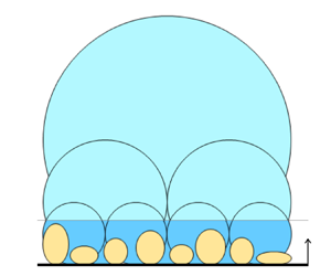
The Navier slip boundary condition (Navier Reference Navier1823) was applied in the streamwise direction, i.e.  ${\tilde{u}_S} = {L_S}(\textrm{d}\tilde{u}/\textrm{d}y){|_{wall}}$, where ũS is the slip velocity, LS is the slip length and ũ is the streamwise velocity. Here, ũ (= U + u) can be decomposed into the streamwise mean velocity (U) and its fluctuations (u). Figure 1 shows the relationships between the streamwise mean velocity, the mean slip velocity (US) and LS. The slip length is fixed at LS = 0.01δ to give a drag reduction rate of 34 % for the channel flow with the no-slip condition (Fukagata, Kasagi & Koumoutsakos Reference Fukagata, Kasagi and Koumoutsakos2006). Consequently, the friction Reynolds numbers (Reτ) for the slip and no-slip cases are 469 and 577, respectively. Details of the numerical procedure and its validation can be found in Yoon et al. (Reference Yoon, Hwang, Lee, Sung and Kim2016b).

Figure 1. Schematic diagram of the streamwise mean velocity (U), where US and LS are the mean slip velocity and slip length, respectively.
2.1. Turbulence statistics
Figure 2 shows the turbulence statistics of turbulent channel flows with slip and no-slip conditions. The quantities are normalized by the wall units of each case. The magnitude of streamwise mean velocity  $({U^ + })$ is larger than that of the no-slip case due to the streamwise slip (figure 2a). The dashed line in figure 2(a) represents the mean velocity relative to the wall
  $({U^ + } - U_S^ + )$ for the slip case, which coincides with the profile of
  ${U^ + }$ for the no-slip case. The mean shear in the wall units
  $(\textrm{d}{U^ + }\textrm{/d}{y^ + })$ is insensitive to the streamwise slip. The streamwise slip induces a virtual origin in U + at
  ${y^ + } =-L_S^ +$, leading to the upward shift of U + as
  $\Delta {U^ + } = U_S^ + = L_S^ + $ in the entire region (García-Mayoral, Gómez-de-Segura & Fairhall Reference García-Mayoral, Gómez-de-Segura and Fairhall2019). The streamwise turbulence intensity
  $(u_{rms}^ + )$ is amplified with respect to that of the no-slip case below y + = 10, especially very close to the wall (figure 2c), due to the streamwise slip. A virtual origin for turbulence is absent due to the combined influences of wall-normal and spanwise slip lengths (Ibrahim et al. Reference Ibrahim, Gómez-de-Segura, Chung and García-Mayoral2021), showing almost the same inner peaks of
  $u_{rms}^ +$ (Kim, Moin & Moser Reference Kim, Moin and Moser1987). In contrast, a profile of Reynolds shear stress
  $({\langle - uv\rangle ^ + })$ is well matched with that for the no-slip case in the inner region as a result of an impermeable condition at the wall. For outer scaling, the profiles of
  $U_c^ +{-} {U^ + }$ (figure 2b),
  $u_{rms}^ +$ and
  ${\langle - uv\rangle ^ + }$ (figure 2d) for both cases collapse well in the outer region, supporting Townsend's outer-layer similarity hypothesis and in agreement with the results of Flores & Jiménez (Reference Flores and Jiménez2006) and Chung et al. (Reference Chung, Monty and Ooi2014). Here, Uc is the mean velocity at the channel centre.

Figure 2. Profiles of (a) mean velocity (U +) and (b) defect form  $(U_c^ +-{U^ + })$ of mean velocity, where Uc is the mean velocity at the channel centre. A dashed line in panel (a) represents mean velocity relative to wall
  $({U^ + }-U_S^ + )$ for the slip case. Profiles of streamwise turbulence intensity
  $(u_{rms}^ + )$ and Reynolds shear stress
  $({\langle - uv\rangle ^ + })$ for (c) inner scaling and (d) outer scaling.
3. Wall-attached structures
3.1. Identification of coherent structures
The 3-D u clusters in instantaneous flow fields can be defined as the groups of connected points satisfying  $u(\boldsymbol{x},t) \ge \alpha {u_{rms}}(y)$ and
  $u(\boldsymbol{x},t) \le - \alpha {u_{rms}}(y)$. Here, α is the threshold, which is selected from the percolation diagram in figure 3(a), and x and t represent the spatial vector and time, respectively. The total number (N) and total volume (V) of u clusters at a given α are normalized by the maximum N (Nmax) and maximum V (Vmax), respectively. As α decreases, new clusters appear or some adjacent clusters merge. The peak in N/Nmax at α = 1.6 results from the tradeoff between these two influences; the former is dominant for α > 1.6 and vice versa. In addition, V/Vmax increases as α decreases with strong variation in the region of 1.4 < α < 1.8, where the percolation transition occurs. Hence, we chose α = 1.6 in the present study.

Figure 3. (a) Percolation diagram for the detected u clusters. Variations with α in the total volume (V) and total number (N) of clusters. (b) Number of u clusters per unit wall-parallel area (n*) with respect to  $y_{min}^ +$ and
  $y_{max}^ +$.
Based on this condition, each u cluster can be detected by using the connectivity of six-orthogonal grids at a given node in Cartesian coordinates (Moisy & Jiménez Reference Moisy and Jiménez2004; del Álamo et al. Reference del Álamo, Jiménez, Zandonade and Moser2006; Lozano-Durán et al. Reference Lozano-Durán, Flores and Jiménez2012; Hwang & Sung Reference Hwang and Sung2018; Lozano-Durán & Bae Reference Lozano-Durán and Bae2019; Hwang et al. Reference Hwang, Lee and Sung2020; Yoon et al. Reference Yoon, Hwang, Yang and Sung2020). As a result, the spatial information for each u cluster can be obtained. The u clusters with volumes less than 303 wall units are discarded to avoid grid resolution (del Álamo et al. Reference del Álamo, Jiménez, Zandonade and Moser2006). Figure 3(b) shows the population density (n*) of all the identified u clusters as functions of ymax and ymin, which are the maximum and minimum distances from the wall, respectively. Here, n* is defined as the number of u clusters (n) per unit wall-parallel area (Axz = LxLz), i.e.  ${n^\ast } = n({y_{max}},{y_{min}})/(m{A_{xz}})$, where m is the number of snapshots (m = 1164 for the slip case and m = 1144 for the no-slip case). Two distinct groups are evident at
  $y_{min}^ +\approx 0$ and
  $y_{min}^ + > 0$, where the former are wall-attached structures and the latter are wall-detached structures (Hwang & Sung Reference Hwang and Sung2018; Yoon et al. Reference Yoon, Hwang, Yang and Sung2020).
The 3-D iso-surfaces of u of wall-attached and wall-detached structures are shown in figure 4(a) for the slip case and in figure 4(b) for the no-slip case. Blue and red correspond to negative u and positive u, respectively. The characteristic length scales of each u cluster can be defined in terms of the dimensions of the box circumscribing the object. The inset in figure 4(a) shows a wall-attached structure and its length scales, i.e. lx, lz and ly, which are the streamwise and spanwise sizes and the height, respectively. As can be seen in figure 4, the wall-attached u structures are coherent in the streamwise direction and aligned side by side in the spanwise direction. At first sight, those for the slip case appear similar respectively to those for the no-slip case. However, upon closer inspection, differences in terms of the population density of the wall-attached structures are observed. The wall-attached structures are sparsely distributed for the slip case. The streamwise slip induces streamwise velocities at the wall (figure 2a) and enhances the magnitude of  $u_{rms}^ +$ near the wall (figure 2c). We can observe sparse wall-attached structures in an instantaneous flow field despite the presence of slip at the wall. The wall-detached structures are less coherent than the wall-attached structures and are randomly distributed in the domain.

Figure 4. 3-D iso-surfaces of the wall-attached and wall-detached u structures in an instantaneous flow field for (a) the slip case and (b) the no-slip case.
3.2. Influences of streamwise slip on wall-attached structures
Figure 5 shows the joint probability density functions (JPDF) of  $l_x^ +$ and
  $l_z^ +$ with respect to
  $l_y^ +$, which is the height of wall-attached structures (ly = ymax,
  $l_y^ +\approx {y^ + }$ because of ymin ≈ 0). Colour and line contours apply to the slip and no-slip cases, respectively. Circles correspond to the mean lengths for the slip (red) and no-slip (black) cases.

Figure 5. Contours of JPDF of (a)  $l_x^ +$ and
  $l_y^ +$ and of (b)
  $l_z^ +$ and
  $l_y^ +$ of wall-attached u structures. The circles are the mean lengths. The green lines in panels (a) and (b) are
  $\langle {l_x}\rangle \sim l_y^{0.74}$ and
  $\langle {l_z}\rangle \sim {l_y}$, respectively.
As shown in figure 5(a), the mean  $l_x^ + (\langle l_x^ + \rangle )$ is proportional to
  $l_y^ +$ with the power of 0.74 (Hwang & Sung Reference Hwang and Sung2018) in the region of
  $l_y^ + \ge 70 \approx 3Re_\tau ^{0.5}$, whereas not proportional to
  $l_y^ + (l_y^ + < 70)$. Here,
  $3Re_\tau ^{0.5}$ is the lower limit of the logarithmic region (Marusic et al. Reference Marusic, Monty, Hultmark and Smits2013; Hwang & Sung Reference Hwang and Sung2019), which accords with approximately 70ν/uτ at the present Reynolds number (Reτ ≈ 500). In addition, there is a linear relationship between the mean
  $l_z^ + (\langle l_z^ + \rangle )$ and
  $l_y^ + (l_y^ + \ge 70)$ (figure 5b), which shows that the spanwise size of wall-attached u structures is proportional to the distance from the wall (Tomkins & Adrian Reference Tomkins and Adrian2003; del Álamo et al. Reference del Álamo, Jiménez, Zandonade and Moser2006; Hwang Reference Hwang2015). In particular, the JPDF of
  $l_x^ +$ and
  $l_z^ +$ with
  $l_y^ +$ for both cases coincide in the entire
  $l_y^ +$ region, especially
  $l_y^ + \ge 70$, in agreement with the results of Lozano-Durán & Bae (Reference Lozano-Durán and Bae2019). Accordingly, we divide wall-attached structures into non-self-similar
  $(l_y^ + < 70)$ and self-similar
  $(l_y^ + \ge 70)$ structures.
The population density  $(n_a^\ast )$ of wall-attached structures with respect to
  $l_y^ +$ is shown in figure 6(a). Here, na is the number of wall-attached structures as a function of their height ly, and the population density
  $(n_a^\ast )$ of wall-attached structures is defined as na per unit wall-parallel area, i.e.
  $n_a^\ast = {n_a}/(m{A_{xz}})$. The magnitude of
  $n_a^\ast $ is smaller than that for the no-slip case in the entire region. The wall-attached structures with the height of
  $l_y^ + = O(10)$ are related to near-wall streaks. As shown in figure 2(a), the mean shear is preserved near the wall for the slip case, sustaining turbulence via the formation process of streaky structures (Hamilton, Kim & Waleffe Reference Hamilton, Kim and Waleffe1995; Waleffe Reference Waleffe1997). The streamwise slip attenuates streamwise vortices near the wall, creating streaks sparsely (Min & Kim Reference Min and Kim2004; Kim Reference Kim2011). The lack of streamwise vortices leads to reduced populations of wall-attached structures near the wall.

Figure 6. (a) Population density  $(n_a^\ast )$ and (b) volumes of wall-attached structures per unit domain volume
  $(V_a^\ast )$ as a function of
  $l_y^ +$. Green lines denote an inverse power-law distribution of
  $n_a^\ast $ in panel (a) and linear variation in
  $V_a^\ast $ in panel (b). Dashed lines in panels (a) and (b) represent
  $l_y^ + = 1.06{\delta ^ + }$ and
  $l_y^ + = 1.13{\delta ^ + }$, respectively.
The magnitude of  $n_a^\ast $ is inversely proportional to
  $l_y^ +$ in the region of
  $250 < l_y^ + < 400$ for both cases, reminiscent of the distribution of hierarchy length scales of attached eddies (Perry & Chong Reference Perry and Chong1982). The inverse power-law dependence arises within the region of
  $l_y^ + = 0.3{\delta ^ + }-0.6{\delta ^ + }$ for zero-pressure-gradient TBL at Reτ ≈ 1000 (Hwang & Sung Reference Hwang and Sung2018) and turbulent pipe flows at Reτ ≈ 1000 and 3000 (Hwang & Sung Reference Hwang and Sung2019). The streamwise slip induces a decrease in the population density of wall-attached structures, but the inverse power law is still valid. The no-slip boundary condition is not indispensable to form hierarchical distributions of wall-attached structures. In addition, a peak in
  $n_a^\ast $ arises at
  $l_y^ + = 1.06{\delta ^ + }$ for both cases, which results from the large population of wall-attached δ-height structures (Perry et al. Reference Perry, Henbest and Chong1986).
In contrast to the variation in  $n_a^\ast $, the magnitude of
  $V_a^\ast $ increases with increasing
  $l_y^ + $ up to
  $l_y^ +\approx {\delta ^ + }$ (figure 6b). Here,
  $V_a^\ast $ is defined as the volume of wall-attached structures per unit domain volume, i.e.
  $V_a^\ast = {V_a}/(m{A_{xz}}\delta )$, where Axzδ is the domain volume. The profiles of
  $V_a^\ast $ for both cases collapse well below
  $l_y^ + = 30$. The magnitude of
  $V_a^\ast $ is even larger than that for the no-slip case in the region of
  $l_y^ + = 30-550$, whereas the number of wall-attached structures is smaller than that for the no-slip case (figure 6a). A peak in
  $V_a^\ast $ arises at
  $l_y^ + = 1.13{\delta ^ + }$ for both cases; this trend is the same as that in
  $n_a^\ast $.
Figure 7 shows wall-normal profiles of streamwise Reynolds stresses  $(\langle uu\rangle _a^{{\ast}{+} })$ carried by the wall-attached structures with the height of
  $l_y^ + = 300$ and 1.06δ +,
 \begin{equation}\langle uu\rangle _a^\ast (y,{l_y}) = \left\langle {{S_a}{{(y,{l_y})}^{ - 1}}\int_{{S_a}} {u(\boldsymbol{x})u(\boldsymbol{x})\,\textrm{d}\kern0.06em x\,\textrm{d}z} } \right\rangle ,\end{equation}
where Sa is the wall-parallel area of wall-attached structures as functions of y and ly. As shown in figure 7(a), the magnitude of  $\langle uu\rangle _a^{{\ast}{+} }$ for
  $l_y^ + = 300$ is logarithmically proportional to y +
  $(\langle uu\rangle _a^{{\ast}{+} }\sim \ln {y^ + })$ in the region of 100 < y + < 220 (Perry & Chong Reference Perry and Chong1982). Although the present Reynolds number is relatively low (Reτ ≈ 500), the logarithmic variation is evident in
  $\langle uu\rangle _a^{{\ast}{+} }$ reconstructed from the wall-attached structures (Hwang & Sung Reference Hwang and Sung2018; Hwang et al. Reference Hwang, Lee and Sung2020; Yoon et al. Reference Yoon, Hwang, Yang and Sung2020). Wall-attached δ-height structures are not self-similar with their height, but contaminate the logarithmic variation in the streamwise Reynolds stress (Hwang et al. Reference Hwang, Lee and Sung2020; Yoon et al. Reference Yoon, Hwang, Yang and Sung2020). Wall-attached δ-height structures are self-similar with ly (figure 5). The profiles of
  $\langle uu\rangle _a^{{\ast}{+} }$ for
  $l_y^ + = 1.06{\delta ^ + }$ are similar to those for
  $l_y^ + = 300$, and the logarithmic variation is still valid in the region of
  $l_y^ + = 100-220$ (figure 7b). The logarithmic behaviour of wall-attached structures is sustained regardless of the streamwise slip at the wall.

Figure 7. Streamwise Reynolds stresses  $(\langle uu\rangle _a^ + )$ reconstructed by wall-attached structures with the height of (a)
  $l_y^ + = 300$ and (b)
  $l_y^ + = 1.06{\delta ^ + }$. Green dashed lines in panel (a) indicate the best fits in the region of 100 < y + < 220:
  $\langle uu\rangle _a^{{\ast}{+} } = 35.73 - 5.14\ln {y^ + }$ for the slip case and
  $\langle uu\rangle _a^{{\ast}{+} } = 36.44 - 5.08\ln {y^ + }$ for the no-slip case, and those in panel (b) are for
  $\langle uu\rangle _a^{{\ast}{+} } = 36.24 - 5.09\ln {y^ + }$ (slip) and
  $\langle uu\rangle _a^{{\ast}{+} } = 34.44 - 4.52\ln {y^ + }$ (no-slip). Two vertical dashed lines represent y + = 100 and y + = 220.
4. Near-wall part of wall-attached self-similar structures
Townsend's attached-eddy hypothesis (Townsend Reference Townsend1976) is useful for the prediction of turbulence statistics in the logarithmic region; coherent structures are constructed through the superposition of attached self-similar eddies. However, careful attention must be paid to the use of attached-eddy models, since Townsend's attached-eddy hypothesis strictly only applies to high-Reynolds-number wall-bounded flows, which are inviscid near the wall. To limit the influence of viscosity on wall-attached structures, the majority of studies have focused on wall-attached structures above the logarithmic region (del Álamo et al. Reference del Álamo, Jiménez, Zandonade and Moser2006; Lozano-Durán et al. Reference Lozano-Durán, Flores and Jiménez2012; Hwang & Sung Reference Hwang and Sung2018; Yoon et al. Reference Yoon, Hwang, Yang and Sung2020). Hwang & Sung (Reference Hwang and Sung2018) observed an inverse power law in the population density  $(290 < l_y^ + < 550)$ of wall-attached structures that is responsible for the logarithmic variation in the streamwise Reynolds stress
  $(3Re_\tau ^{0.5} < {y^ + } < 0.18{\delta ^ + })$. Wall-attached structures with
  $3Re_\tau ^{0.5} \le l_y^ + \le 0.6{\delta ^ + }$ are self-similar with their height (Hwang et al. Reference Hwang, Lee and Sung2020).
4.1. Structural features
The characteristics of wall-attached structures can be divided into buffer-layer  $(l_y^ + < 70 \approx 3Re_\tau ^{0.5})$ and self-similar
  $(l_y^ + \ge 70)$ structures. As shown in figure 5, the upper part
  $({y^ + } \ge 70)$ of WASS
  $(l_y^ + \ge 70)$ is responsible for the logarithmic behaviour (figure 7b). The near-wall part (y + < 70) of WASS
  $(l_y^ + \ge 70)$ contributes to geometrical self-similarity (figure 5). The wall-attached structures can be decomposed into unws, uuws and uwb, which are defined as
 \begin{gather}{u_{nws}}(\boldsymbol{x}) = \left\{ {\begin{array}{*{20}{l}} u&{\textrm{if}\;|u|\ge 1.6{u_{rms}},\;y_{min}^ +\approx 0,\;y_{max}^ + \ge 70,\;{y^ + } < 70,}\\ 0&{\textrm{otherwise,}} \end{array}} \right.\end{gather}
 \begin{gather}{u_{uws}}(\boldsymbol{x}) = \left\{ {\begin{array}{*{20}{l}} u&{\textrm{if}\;|u|\ge 1.6{u_{rms}},\;y_{min}^ +\approx 0,\;y_{max}^ + \ge 70,\;{y^ + } \ge 70,}\\ 0&{\textrm{otherwise,}} \end{array}} \right.\end{gather}
 \begin{gather}{u_{wb}}(\boldsymbol{x}) = \left\{ {\begin{array}{*{20}{l}} u&{\textrm{if}\;|u|\ge 1.6{u_{rms}},\;y_{min}^ +\approx 0,\;y_{max}^ + < 70,}\\ 0&{\textrm{otherwise}.} \end{array}} \right.\end{gather}
Here, the subscripts ‘nws’, ‘uws’ and ‘wb’ represent the near-wall part of WASS, upper part of WASS and wall-attached buffer-layer structures (WABS), respectively. From now on, we focus on the near-wall part of WASS, in which the viscosity effect is dominant.
Figure 8 illustrates 3-D iso-surfaces of u wall-attached structures for the no-slip case in an instantaneous flow field. Red and blue correspond to positive u and negative u, respectively. A schematic diagram in the inset of figure 9 helps to understand the decomposition of wall-attached structures: upper-part of self-similar, near-wall part of self-similar and buffer layer. Note that both unws and uwb are located in the region of y + < 70. The near-wall part of WASS is more coherent than the WABS. In addition, the near-wall part of WASS (y + < 70) is easily observed in an instantaneous flow field, interpreted as the footprints of large-scale motions (Hutchins & Marusic Reference Hutchins and Marusic2007; Hwang et al. Reference Hwang, Lee, Sung and Zaki2016).

Figure 8. 3-D iso-surfaces of u wall-attached structures: self-similar  $(l_y^ + \ge 70 \approx 3Re_\tau ^{0.5})$; the upper part (uuws) (
 $l_y^ + \ge 70$ and y + ≥ 70) and near-wall part (unws) (
 $l_y^ + \ge 70$ and y + < 70) and buffer-layer
  $(u_{wb}) (l_y^ + < 70)$. Red and blue correspond to positive u and negative u, respectively.

Figure 9. Two-point correlations of (a) unws and (b) uwb. The reference wall-normal location is  $y_{ref}^ + = 14.5$. Solid lines represent 5 % of the maximum of positive correlations, and dashed lines denote 50 % of the minimum of negative correlations. Cross symbols indicate spanwise centres of negative correlations. The blue line in panel (a) accords with R[uwb, uwb] for the slip case in panel (b).
To investigate sizes of the near-wall part of WASS statistically, conditional two-point correlations of unws are examined at the reference wall-normal location  $y_{ref}^ + = 14.5$, where the inner peak arises in
  $u_{rms}^ + $ (figure 2c). The two-point correlations of unws and uwb are defined as
 \begin{gather}R[{u_{nws}},{u_{nws}}]({r_x},y,{r_z},{y_{ref}}) = \frac{{\langle {u_{nws}}(x,{y_{ref}},z){u_{nws}}(x + {r_x},y,z + {r_z})\rangle }}{{{u_{nws,\,rms}}({y_{ref}}){u_{nws,\,rms}}(y)}},\end{gather}
 \begin{gather}R[{u_{wb}},{u_{wb}}]({r_x},y,{r_z},{y_{ref}}) = \frac{{\langle {u_{wb}}(x,{y_{ref}},z){u_{wb}}(x + {r_x},y,z + {r_z})\rangle }}{{{u_{wb,\,rms}}({y_{ref}}){u_{wb,\,rms}}(y)}},\end{gather}
where unws,rms and uwb,rms are the root-mean-square quantities of unws and uwb, respectively. For comparison, the two-point correlation of uwb is included.
Wall-parallel views of R[unws, unws] are shown in figure 9(a), where solid and dashed lines denote 5 % of the maximum of positive R[unws, unws] and 50 % of the minimum of negative R[unws, unws], respectively. The positive R[unws, unws] are extended to approximately 4.3δ in the streamwise direction, which is similar to streamwise lengths of the footprints of large-scale motions at the same location of  $y_{ref}^ +\approx 14.5$ (Lee & Sung Reference Lee and Sung2013; Hwang et al. Reference Hwang, Lee, Sung and Zaki2016; Yoon et al. Reference Yoon, Hwang, Lee, Sung and Kim2016b; Hwang & Sung Reference Hwang and Sung2017). In addition, the scaling of negative R[unws, unws] with δ indicates that the near-wall part of WASS is aligned side by side along the spanwise direction. The distance to the centre (cross symbol) of negative R[unws, unws] at rx = 0 is 0.6δ, which is 20 % larger than that for the no-slip case. This result represents that the near-wall part of WASS is more sparsely distributed than those for the no-slip case (figure 4).
Figure 9(b) shows line contours of R[uwb, uwb] in the x–z plane. Compared to R[unws, unws], the negative R[uwb, uwb] is not observed, representing that the WABS are not influenced by adjacent other WABS. This is consistent with the observations in figure 8, where iso-surfaces of uwb are more sparsely populated than those of unws. The line contour of R[uwb, uwb] is transversely away from the reference centre (rx = 0 and rz = 0) by 85v/uτ, implying that the WABS are closely related to the near-wall streaks (Kline et al. Reference Kline, Reynolds, Schraub and Runstadler1967). The streamwise extension of positive R[uwb, uwb] is 500ν/uτ at rz = 0, which is 7.7 % longer than that for the no-slip case. The blue contour in figure 9(a) represents R[uwb, uwb] for the slip case, indicating that the WABS are much shorter in the streamwise direction than the near-wall part of WASS.
To further examine geometrical features of the near-wall part of WASS, two-point correlations of ua (R[ua, ua]) at a given ly are performed at  $y_{ref}^ + = 14.5$. The conditional field (ua) and two-point correlation of ua are defined as
 \begin{equation}{u_a}(\boldsymbol{x},{l_y}) = \left\{ {\begin{array}{*{20}{l}} u&{\textrm{if}\;|u|\ge 1.6{u_{rms}},\;y_{min}^ +\approx 0,}\\ 0&{\textrm{otherwise},} \end{array}} \right.\end{equation}
 \begin{equation}R[{u_a},{u_a}]({r_x},y,{r_z},{y_{ref}},{l_y}) = \frac{{\langle {u_a}(x,{y_{ref}},z,{l_y}){u_a}(x + {r_x},y,z + {r_z},{l_y})\rangle }}{{{u_{a,\,rms}}({y_{ref}},{l_y}){u_{a,\,rms}}(y,{l_y})}},\end{equation}
where ua,rms is the root-mean-square quantity of ua. Figure 10(a) shows the x–z plane (at  ${y^ + } = y_{ref}^ +$) and x–y plane (at
  $r_z^ + = 0$) views of R[ua, ua] for
  $l_y^ + = 300$. The wall-attached structures with the height of
  $l_y^ + = 300$ are more stretched in both upstream and downstream directions than those for the no-slip case. These observations support that weakened wall-shear stress due to the streamwise slip results in a long extension of wall-attached structures to the wall (Chung et al. Reference Chung, Monty and Ooi2014).

Figure 10. (a) Two-point correlations of ua for  $l_y^ + = 300$ in the x–y and x–z planes. The reference wall-normal location is
  $y_{ref}^ + = 14.5$. Line contours are R[ua, ua] = 0.05. (b) Streamwise and spanwise characteristic lengths (
 $R_x^ +$ and
  $R_z^ +$) of the near-wall part of WASS at
  $y_{ref}^ + = 14.5$ with respect to
  $l_y^ +$.
Figure 10(b) shows characteristic length scales of the near-wall part of WASS at  $y_{ref}^ + = 14.5$. Their streamwise and spanwise lengths (Rx and Rz) can be defined in terms of the difference between the streamwise and spanwise displacements at
  $R[{u_a},{u_a}](r_x^ + ,{y^ + } = y_{ref}^ + ,r_z^ + = 0) = 0.05$ and
  $R[{u_a},{u_a}](r_x^ + = 0,{y^ + } = y_{ref}^ + ,r_z^ + ) = 0.05$, respectively. The magnitude of
  $R_x^ +$ and
  $R_z^ +$ gradually increases for both cases with the increase in
  $l_y^ +$. Interestingly, streamwise lengths of the near-wall part of WASS are longer than those for the no-slip case, and vice versa for the spanwise lengths up to
  $l_y^ + = 600$. The magnitude of
  $R_x^ +$ is larger than 1δ +, and is thus related to the footprints of large-scale motions (Hutchins & Marusic Reference Hutchins and Marusic2007). The magnitude of
  $R_x^ +$ is approximately 1.3 times larger than that for the no-slip case up to
  $l_y^ + = 400$, over which the difference in
  $R_x^ +$ between two cases becomes larger. Although sizes of WASS are independent of the streamwise slip (figure 5), their roots are stretched and compressed in the streamwise and spanwise directions, respectively.
4.2. Conditional statistics
We investigate the turbulence statistics of the near-wall part of WASS along the wall-normal location. The turbulence statistics for the near-wall part of WASS can be conditionally averaged based on conditional fields, where velocity and vorticity fluctuations are obtained using equations similar to (4.1a). Conditionally averaged quantities are used to assess contributions of the near-wall part of WASS to the turbulence statistics in the region of y + < 70.
Figure 11 introduces wall-normal profiles of conditional averages for the near-wall part of WASS. Profiles of Anws/Axz (figure 11a) represent wall-parallel areas occupied by the near-wall part of WASS, which account for 5–7 % of the area of the x–z plane. Below y + = 30, the magnitude of Anws/Axz is larger than that for the no-slip case, in particular, 74.3 % larger near the wall. The streamwise slip induces long tails, observed from the conditional two-point correlations (figure 10a). Similar results were reported from the footprints of large-scale motions by a streamwise slip (Yoon et al. Reference Yoon, Hwang, Lee, Sung and Kim2016b). As shown in figure 11(b), the magnitude of  $\langle uu\rangle _{nws}^ + $ is larger than that for the no-slip case below y + = 30, which indicates that the near-wall part of WASS is strengthened by the streamwise slip.

Figure 11. Conditionally averaged turbulence statistics of the near-wall part of WASS: wall-normal profiles of (a) Anws/Axz, (b)  $\langle uu\rangle _{nws}^ + $, (c)
  $\langle - uv\rangle _{nws}^ + $ and (d)
  $\textrm{d}U_{nws}^ +{/}\textrm{d}{y^ + }$.
In contrast to  $\langle uu\rangle _{nws}^ + $, profiles of
  $\langle - uv\rangle _{nws}^ + $ for both cases collapse (figure 11c), similar to
  ${\langle - uv\rangle ^ + }$ (figure 2a). The streamwise slip results in the enhancement of negative unws and the attenuation of vnws from the weighted JPDF of
  $u_{nws}^ + v_{nws}^ + $ (not shown here). Accordingly, the magnitudes
  $\langle - uv\rangle _{nws}^ + $ for both cases are similar. The near-wall part of WASS contributes to approximately 30 % of the total
  $\langle - uv\rangle $ despite of a small Anws/Axz (figure 11c), representing that they are the main energy-containing motions near the wall. Figure 11(d) shows the mean shear
  $(\textrm{d}U_{nws}^ + \textrm{/d}{y^ + })$ carried by the near-wall part of WASS. Below y + = 20, the magnitude of
  $\textrm{d}U_{nws}^ + \textrm{/d}{y^ + }$ is larger than that for the no-slip case, especially by 9 % in the vicinity of the wall. The magnitude of
  $\textrm{d}U_{nws}^ +{/}\textrm{d}{y^ + }$ at the wall can be interpreted as the ratio τw,nws/τw, where τw,nws is the wall shear stress carried by the near-wall part of WASS. Given that the wall shear stress is related to the skin friction coefficient, the high
  $\textrm{d}U_{nws}^ +{/}\textrm{d}{y^ + }$ at the wall is responsible for the frictional drag. The majority of discrepancy in
  $\textrm{d}U_{nws}^ +{/}\textrm{d}{y^ + }$ comes from the high Anws/Axz (figure 11a). The mean shear of the near-wall part of WASS for the slip case is restored above y + = 30. In contrast to the upper part of WASS, the near-wall part of WASS can be varied by the viscosity and wall conditions, but their contributions to the streamwise Reynolds stress and Reynolds shear stress are more significant.
Two velocity–vorticity correlations  $({\langle v{\omega _z}\rangle _{nws}}$ and
  ${\langle - w{\omega _y}\rangle _{nws}})$ carried by the near-wall part of WASS are plotted in figure 12(a,c). The former is related to the advective vorticity transport, and the latter represents the vortex stretching (Tennekes & Lumley Reference Tennekes and Lumley1972). Here, ωz and ωy are the spanwise and wall-normal vorticity fluctuations, respectively. In addition, these velocity–vorticity correlations are important to near-wall turbulence, since they are directly related to the frictional drag (Yoon et al. Reference Yoon, Ahn, Hwang and Sung2016a; Hwang & Sung Reference Hwang and Sung2017; Yoon, Hwang & Sung Reference Yoon, Hwang and Sung2018). The magnitude of
  $\langle v{\omega _z}\rangle _{nws}^ + $ is significantly reduced near the positive peak at y + = 4.5 (figure 12a). Figure 12(b) shows the weighted JPDF of
  $v_{nws}^ + \omega _{z,nws}^ + $ at y + = 4.5, where
  $\langle v{\omega _z}\rangle _{nws}^ + $ has a positive peak (figure 12a). At the first quadrant
  $({v_{nws}} > 0\;\& \;{\omega _{z,nws}} > 0)$, the magnitude of mean
  $\omega _{z,nws}^ + $ is 28.2 % smaller than that for the no-slip case, and the magnitude of mean
  $v_{nws}^ + $ decreases by 18.4 %. The first quadrant of the weighted JPDF of vωz at a positive peak of
  $\langle v{\omega _z}\rangle $ is interpreted as the vertical advection of sublayer streaks (Klewicki, Murray & Falco Reference Klewicki, Murray and Falco1994; Chin et al. Reference Chin, Philip, Klewicki, Ooi and Marusic2014). Both the weakened near-wall part of WASS and upward motions lead to the reduction in positive
  $\langle v{\omega _z}\rangle _{nws}^ + $. In addition, a peak is evident in the negative
  $\langle v{\omega _z}\rangle _{nws}^ + $ at y + = 30, whereas a negative peak of
  ${\langle v{\omega _z}\rangle ^ + }$ is observed at y + = 18 (not shown here), corresponding to outward motions of hairpin vortex heads (Klewicki et al. Reference Klewicki, Murray and Falco1994; Chin et al. Reference Chin, Philip, Klewicki, Ooi and Marusic2014). Given that vortical structures are in the form surrounding streaky structures (Adrian, Meinhart & Tomkins Reference Adrian, Meinhart and Tomkins2000; Lee & Sung Reference Lee and Sung2009; Dennis & Nickels Reference Dennis and Nickels2011), the conditional field for the near-wall part of WASS does not fully form hairpin-like vortical structures.

Figure 12. Profiles of velocity–vorticity correlations carried by near-wall part of WASS: (a)  $\langle v{\omega _z}\rangle _{nws}^ + $ and (c)
  $\langle - w{\omega _y}\rangle _{nws}^ + $. Weighted JPDF of (b)
  $v_{nws}^ + \omega _{z,nws}^ + $ at y + = 4.5 and (d)
  $w_{nws}^ + \omega _{y,nws}^ + $ at y + = 7.0. The solid and dashed lines correspond to positive and negative values, respectively. Contours are from −0.002 to +0.002 with increments of 0.001.
Figure 12(c) shows wall-normal profiles of  $\langle - w{\omega _y}\rangle _{nws}^ + $, in which a positive peak is evident at y + = 7 and positive values are present up to y + = 50. The positive
  $\langle - w{\omega _y}\rangle $ are physically related to the simultaneous collapse of two adjacent hairpin vortex legs, leading to the stretching of hairpin vortices (Eyink Reference Eyink2008; Chin et al. Reference Chin, Philip, Klewicki, Ooi and Marusic2014). The magnitude of
  $\langle - w{\omega _y}\rangle _{nws}^ +$ is similar to that for the no-slip case. Figure 12(d) represents the weighted JPDF of
  $w_{nws}^ + \omega _{y,nws}^ + $ at y + = 7, where two motions with negative correlations (wnws > 0 and ωy,nws < 0, and wnws < 0 and ωy,nws > 0) are dominant. Although the magnitudes of mean
  $w_{nws}^ + $ and mean
  $\omega _{y,nws}^ + $ at negative correlations are 25 % and 13 % smaller than those for the no-slip case, the magnitude of
  ${\langle - w{\omega _y}\rangle ^ + }$ at y + = 7 is similar to each other due to higher population density of negative correlations. The energy transfer via vortex stretching of the near-wall part of WASS is attenuated by the streamwise slip.
To determine the turbulence statistics reconstructed by the wall-attached structures at a given height, the streamwise velocity and its wall-normal gradient are conditionally averaged as a function of ly,
 \begin{gather}{U_a}({l_y}) = \left\langle {{V_a}{{({l_y})}^{ - 1}}\int_{{V_a}} {\tilde{u}(\boldsymbol{x})\,\textrm{d}\boldsymbol{x}} } \right\rangle ,\end{gather}
 \begin{gather}\frac{{\textrm{d}{U_a}}}{{\textrm{d}y}}({l_y}) = \left\langle {{V_a}{{({l_y})}^{ - 1}}\int_{{V_a}} {\frac{{\textrm{d}\tilde{u}(\boldsymbol{x})}}{{\textrm{d}y}}\,\textrm{d}\boldsymbol{x}} } \right\rangle .\end{gather}
Figure 13(a) shows the variation in  $U_a^ +$ with
  $l_y^ +$, i.e. the convection velocity of wall-attached structures at a given ly. A large difference in
  $U_a^ +$ is observed at
  $l_y^ + < 30$, while the magnitude of
  $U_a^ +$ is similar in the region of
  $l_y^ + \ge 0.45{\delta ^ + }$. The discrepancy in
  $U_a^ +$ at lower
  $l_y^ +$ is mainly due to the slip velocity at the wall. Interestingly, the difference in
  $U_a^ +$ decreases as
  $l_y^ +$ increases. The wall-attached structures slide in the streamwise direction, leading to the increase in their volume close to the wall (figure 10a). As
  $l_y^ +$ increases, the convection velocity of wall-attached structures gets close to that for the no-slip case.

Figure 13. Profiles of (a) the convection velocity  $(U_a^ + )$ and (b) the mean shear
  $(\textrm{d}U_a^ +{/}\textrm{d}{y^ + })$ carried by wall-attached structures.
The mean shear  $(\textrm{d}U_a^ +{/}\textrm{d}{y^ + })$ carried by the wall-attached structures at a given ly is shown in figure 13(b); it is suppressed in the region of
  $l_y^ + < 50$. Given that the mean shear is directly related to the formation of near-wall streaks (Waleffe Reference Waleffe1997), the weakened mean shear results in a lower population density of WABS for the slip case (figure 6a). However, profiles of
  $\textrm{d}U_a^ +{/}\textrm{d}{y^ + }$ for both cases collapse well over
  $l_y^ + < 70$, while the lower population of WASS is observed for the slip case, as shown in figure 6(a). This inconsistency reveals that the formation of WASS is affected by the population of WABS (not by the mean shear), supporting the hierarchical distributions of wall-attached structures (Perry & Chong Reference Perry and Chong1982).
To explore the characteristics of the near-wall part of WASS with respect to their height at the near-wall region, conditional averages of wall-parallel area, streamwise velocity, streamwise Reynolds stress and Reynolds shear stress at y + = 14.5 are examined, which are defined as
 \begin{gather}{S_{a,i}}({l_y}) = {S_a}(y,{l_y}){|_{{y^ + } = 14.5}}/(m{A_{xz}}),\end{gather}
 \begin{gather}{U_{a,i}}({l_y}) = U_a^\ast (y,{l_y}){|_{{y^ + } = 14.5}}/U(y){|_{{y^ + } = 14.5}},\end{gather}
 \begin{gather}{\langle uu\rangle _{a,i}}({l_y}) = \langle uu\rangle _a^\ast (y,{l_y}){|_{{y^ + } = 14.5}}/\langle uu\rangle (y){|_{{y^ + } = 14.5}},\end{gather}
 \begin{gather}{\langle - uv\rangle _{a,i}}({l_y}) = \langle - uv\rangle _a^\ast (y,{l_y}){|_{{y^ + } = 14.5}}/\langle - uv\rangle (y){|_{{y^ + } = 14.5}}.\end{gather}
Figure 14(a) shows profiles of the areas in the x–z plane (Sa,i) occupied by the near-wall part of WASS at y + = 14.5. The magnitude of Sa,i gradually decreases as  $l_y^ +$ increases with a peak at
  $l_y^ + = 1.1{\delta ^ + }$. The quantities of Ua,i,
  ${\langle uu\rangle _{a,i}}$ and
  ${\langle - uv\rangle _{a,i}}$ describe the dependence on the height of the near-wall part of WASS in their contributions to the turbulence statistics (i.e. U,
  $\langle uu\rangle $ and
  $\langle - uv\rangle $) at y + = 14.5. Figure 14(b) represents profiles of Ua,i with respect to
  $l_y^ +$, defined as the convection velocity
  $(U_a^\ast )$ of the near-wall part of WASS normalized by U + at y + = 14.5. The region of
  $l_y^ +$, where the magnitude of Ua,i is larger than 1, indicates that positive u of the near-wall part of WASS at a given
  $l_y^ +$ is dominant near y + = 14.5, and vice versa. A peak of Ua,i is observed at
  $l_y^ + = 310$ (slip) and 370 (no-slip), and a concave peak of Ua,i is evident at
  $l_y^ + = 1.12{\delta ^ + }$. In particular, the profile of Ua,i is shifted downward from that for the no-slip case, especially in the region of
  $l_y^ + = 300 - {\delta ^ + }$. It shows that the population of wall-attached negative-u structures with
  $l_y^ +\approx {\delta ^ + }$ are more dominant than that for the no-slip case. These observations are consistent with the dominance of negative-u large-scale motions in the outer region (Yoon et al. Reference Yoon, Hwang, Lee, Sung and Kim2016b).

Figure 14. Conditional averages of the near-wall part of WASS at y + = 14.5: (a) Sa,i; (b) Ua,i; (c)  ${\langle uu\rangle _{a,i}}$ and (d)
  ${\langle - uv\rangle _{a,i}}$. Dashed lines in panels (a) and (b) represent
  $l_y^ + = 1.1{\delta ^ + }$ and 1.12δ +, respectively. A green line in panel (c) denotes the logarithmic variation:
  ${\langle uu\rangle _{a,i}} = 0.089\ln l_y^ +{+} 3.38$.
We now examine the streamwise Reynolds stress  $({\langle uu\rangle _{a,i}})$ at y + = 14.5. Figure 14(c) shows the variation in
  ${\langle uu\rangle _{a,i}}$ with
  $l_y^ +$. The magnitude of
  ${\langle uu\rangle _{a,i}}$ gradually increases with increasing
  $l_y^ +$. The contributions of the near-wall part of WASS to the streamwise Reynolds stress are enhanced as
  $l_y^ +$ increases. In particular, the magnitude of
  ${\langle uu\rangle _{a,i}}$ is logarithmically proportional to
  $l_y^ +$ in the region of
  $100 < l_y^ + < 350\,({\langle uu\rangle _{a,i}}\sim \ln l_y^ + )$ (a green line in figure 15c). The inner-peak magnitude of streamwise Reynolds stress logarithmically increases with increasing Reτ (Jiménez & Hoyas Reference Jiménez and Hoyas2008; Marusic, Baars & Hutchins Reference Marusic, Baars and Hutchins2017). Since ly is related to hierarchical scales (figure 7a), the logarithmic variation in
  ${\langle uu\rangle _a}$ with respect to ly reflects the hierarchical features of wall-attached structures (Hwang & Sung Reference Hwang and Sung2018); this logarithmic variation in
  ${\langle uu\rangle _a}$ is evident in the region of
  $200 < l_y^ + < 300$. A hierarchy of wall-attached structures is well established over the broader range of ly.

Figure 15. Profiles of (a) pre-multiplied  ${\zeta _{2a}}$ and (b) the density of skin friction
  $({\zeta ^{\prime}_{2a}})$ with respect to
  $l_y^ +$. Dashed lines represent
  $l_y^ + = 1.13{\delta ^ + }$. Open symbols in panel (b) represent
  ${\zeta ^{\prime}_{2a, - 34\,\%}}$.
Figure 14(d) shows profiles of  ${\langle - uv\rangle _{a,i}}$, of which the value is larger than 3 in the region of
  $l_y^ + < {\delta ^ + }$. It means that the near-wall part of WASS carry three times more Reynolds shear stresses than
  $\langle - uv\rangle $ in the near-wall region (y + = 14.5). The magnitude of
  ${\langle - uv\rangle _{a,i}}$ is larger than that for the no-slip case below
  $l_y^ + < {\delta ^ + }$. These observations imply that the contributions of the near-wall part of WASS to the near-wall turbulence are dominant, since the Reynolds shear stress is directly related to turbulent contributions to the skin friction coefficient (Fukagata, Iwamoto & Kasagi Reference Fukagata, Iwamoto and Kasagi2002).
5. Decomposition of Cf
The magnitude of the skin friction coefficient (Cf) is 0.0062 for the no-slip case and 0.0041 for the slip case. Drag reduction can be estimated as  $DR = 1 - {[1/(1 + \Delta {U^ + }/U_b^ + )]^2}$ (García-Mayoral et al. Reference García-Mayoral, Gómez-de-Segura and Fairhall2019). The Cf is decomposed into laminar and turbulent components to investigate contributions of wall-attached structures to the frictional drag by using the FIK identity (Fukagata et al. Reference Fukagata, Iwamoto and Kasagi2002) as below:
 \begin{equation}{C_f} = \frac{{2u_\tau ^2}}{{U_b^2}} = \underbrace{{\frac{6}{{R{e_b}}} - \frac{{6{U_S}}}{{R{e_b}{U_b}}}}}_{{ = {C_{f,1}}}} + \underbrace{{\int_0^1 {\frac{6}{{U_b^2}}(1 - y)\langle - uv\rangle \,} \textrm{d}y}}_{{ = {C_{f,2}}}},\end{equation}
where Cf ,1 and Cf ,2 are laminar and turbulent terms, respectively. The majority of Cf is produced by Cf ,2; Cf ,1 contributes approximately 10 % of the overall Cf (Yoon et al. Reference Yoon, Hwang, Lee, Sung and Kim2016b).
5.1. Wall-attached structures
The turbulent term (Cf ,2) can be divided into contributions of wall-attached structures (Cf ,2a) and others (Cf ,2others), which captures contributions of wall-detached structures  $(y_{min}^ + > 0)$ and weak turbulence
  $(-1.6{u_{rms}} < u < 1.6{u_{rms}})$ to Cf ,2. The contribution of wall-attached structures to Cf ,2 can be obtained from the conditional fields:
 \begin{equation}{C_{f,2a}} = \int_{ - \infty }^\infty {{l_y}{\zeta _{2a}}({l_y})\,\textrm{d}\ln {l_y}} ,\quad \textrm{where}\;{\zeta _{2a}}({l_y}) = \frac{6}{{U_b^2}}\left\langle {\int_{{V_a}} { - (1 - y)u(\boldsymbol{x})v(\boldsymbol{x})\,\textrm{d}\boldsymbol{x}} } \right\rangle .\end{equation}
Here,  ${l_y}{\zeta _{2a}}$ as a function of ly is the integrand of Cf ,2a.
Profiles of  $l_y^ + {\zeta _{2a}}$ are plotted on a semi-logarithmic scale in figure 15(a), where the area of profiles is proportional to Cf ,2a. Those profiles are biased towards higher
  $l_y^ +$, and peaks are evident at
  $l_y^ + = 1.13{\delta ^ + }$, representing that wall-attached δ-height structures make the dominant contributions to the frictional drag. The area of
  $l_y^ + {\zeta _{2a}}$ in the region of
  $l_y^ + \ge 70$ is the same as 97 % of the total area, showing that wall-attached structures with
  $l_y^ + \ge 70$ are responsible for almost all of the overall Cf ,2a.
To determine the contributions of wall-attached structures at a given ly to the frictional drag, the density of skin friction  $({\zeta ^{\prime}_{2a}})$ is defined as
 \begin{equation}{\zeta ^{\prime}_{2a}}({l_y}) = {\zeta _{2a}}({l_y})\frac{{m{A_{xz}}\delta }}{{{n_a}{V_a}}}.\end{equation}
Figure 15(b) shows the profile of  ${\zeta ^{\prime}_{2a}}$ with respect to
  $l_y^ +$. A smooth peak in
  ${\zeta ^{\prime}_{2a}}$ is evident at
  $l_y^ + = 100$, which indicates that the wall-attached structures with the height of
  $l_y^ +\approx 100$ contain the highest density of skin friction. The magnitude of
  ${\zeta ^{\prime}_{2a}}$ is more than four times larger than Cf beyond
  $l_y^ + = 30$, in particular, nine times larger near
  $l_y^ + = 100$. This means that each wall-attached structure is responsible for the generation of turbulent frictional drag (de Giovanetti, Hwang & Choi Reference de Giovanetti, Hwang and Choi2016). Open symbols in figure 15(b) represent
  ${\zeta ^{\prime}_{2a, - 34\,\%}}$. The profile of
  ${\zeta ^{\prime}_{\textrm{2}a, - 34\,\%}}$ is shifted downward by as much as 34 % from
  ${\zeta ^{\prime}_{2a}}$. The magnitude of
  ${\zeta ^{\prime}_{2a}}$ at
  $l_y^ + = 1.13{\delta ^ + }$ (red dashed line) is similar to that of
  ${\zeta ^{\prime}_{\textrm{2}a, - 34\,\%}}$ (grey dashed line), representing that the density of skin friction of wall-attached structures with
  $l_y^ + = 1.13{\delta ^ + }$ is similar for both cases. The large difference in
  $l_y^ + {\zeta _{2a}}$ at
  $l_y^ + = 1.13{\delta ^ + }$ (figure 15a) is caused by the volume of wall-attached δ-height structures (figure 6b). The magnitude of
  ${\zeta ^{\prime}_{2a}}$ is 34 % smaller than that of
  ${\zeta ^{\prime}_{2a}}$ for the no-slip case, especially 44 % in the region of
  $250 < l_y^ + < 400$.
5.2. Near-wall part of wall-attached self-similar structures
To scrutinize contributions of the near-wall part of WASS to the skin friction in detail, the turbulent component of Cf is conditionally averaged as functions of y and ly,
 \begin{gather}C_{f,2a}^\ast (y,{l_y}) = \frac{6}{{U_b^2}}\left\langle {\int_{{S_a}} { - (1 - y)u(\boldsymbol{x})v(\boldsymbol{x})\,\textrm{d}\kern0.06em x\,\textrm{d}z} } \right\rangle ,\end{gather}
 \begin{gather}{C_{f,i}}({l_y}) = C_{f,2a}^\ast (y,{l_y}){|_{{y^ + } = 14.5}}/C_{f,2}^\ast (y){|_{{y^ + } = 14.5}},\end{gather}
where  $C_{f,2}^\ast $ is the integrand of Cf ,2 in (5.2) and the double integration of
  $C_{f,2a}^\ast $ with respect to y and ly is the same as Cf ,2a.
Figure 16 shows Cf ,i with respect to  $l_y^ +$, where the area of Cf ,i is proportional to the contribution of the near-wall part of WASS to
  $C_{f,2}^\ast $ at y + = 14.5. The magnitude of Cf ,i exponentially decreases with the increase in
  $l_y^ +$. A smooth peak is observed at
  $l_y^ + = 1.1{\delta ^ + }$, where Sa,i exhibits a large peak (figure 14a). Dominant contributions of the near-wall part of wall-attached δ-height structures to Cf ,2 result from their large area. The contribution of the near-wall part to Cf ,2 in the region of
  $l_y^ + < 400$ is greater than for the no-slip case, although Sa,i is similar below
  $l_y^ + = 400$ (figure 14a). This is due to the enhanced streamwise Reynolds stress and Reynolds shear stress in the vicinity of the wall (figure 14c,d). The near-wall part of WASS is responsible for 19.1 % of
  $C_{f,2}^\ast {\textrm{|}_{{y^ + } = 14.5}}$, which is larger than the no-slip case (17.3 %). Although the near-wall part of WASS occupy only a small area, i.e. approximately 6.3 % of the x–z plane area at y + = 14.5 (figure 11a), its contributions to the skin frictional drag for turbulence are much larger than others.

Figure 16. Profiles of pre-multiplied Cf ,i versus  $l_y^ +$. Dashed lines denote
  $l_y^ + = 1.1{\delta ^ + }$.
6. Conclusions
We have explored wall-attached u structures in a drag-reduced turbulent channel flow and demonstrated their contributions to the frictional drag and near-wall turbulence. We extracted 3-D u clusters by using the connectivity of six-orthogonal neighbours in Cartesian coordinates from the DNS dataset for turbulent channel flows with a Navier slip wall (Reτ = 470) and no-slip wall (Reτ = 577). We showed that wall-attached structures are formed in their entirety in instantaneous flow fields on the wall with the streamwise slip. The wall-attached structures with the height of  $l_y^ + \ge 70 \approx 3Re_\tau ^{0.5}$ were self-similar with ly, and their geometrical features remained unchanged regardless of the streamwise slip. The hierarchical distribution with an inverse power law and the logarithmic behaviour of WASS were also unaffected by the streamwise slip. Influences of the disturbances by the streamwise slip on the wall-attached structures were limited up to the lower bound
  $({y^ + } = 3Re_\tau ^{0.5})$ of the logarithmic region. The streamwise slip induced the decrease in the population density of WABS with weakened mean shear. Given that a hierarchy of WASS was sustained, the decrease in the population density of WASS is attributed to that of WABS, whereas the space occupied by WASS in the fluid domain is enlarged. In addition, we focused on the near-wall part (y + < 70) of WASS
  $(l_y^ + \ge 70)$, and the WABS
  $(l_y^ + < 70)$ were compared. To this end, the conditional average and conditional fields were employed. The near-wall part of WASS was extended in the streamwise direction over 3δ, reminiscent of the footprints of large-scale motions. The near-wall part of WASS contributed to approximately 30 % of the Reynolds shear stress and a quarter of the streamwise Reynolds stress. Next, the skin friction coefficient was decomposed by using the FIK identity to quantify the contributions of wall-attached structures to the frictional drag. The density of skin friction of WASS was more than three-times larger than the magnitude of overall Cf. In addition, the near-wall part of WASS was responsible for approximately 20 % of the turbulent contribution to Cf in the near-wall region despite of the lower volume (5–7 % of total space). The Reynolds shear stress carried by the near-wall part of WASS was enhanced by the streamwise slip, and its contribution to the frictional drag was significant. The streamwise slip curtailed the population density of WASS and the density of skin friction of WASS. The present study enhances our understanding of the behaviour of wall-attached structures and furthers the development of attached-eddy models of drag-reduced flows.
Funding
This work was supported by the National Research Foundation of Korea (NRF) grant funded by the Korea government (MSIT) (No. 2020R1A2C2008106 and 2021R1F1A1053438).
Declaration of interests
The authors report no conflict of interest.


