


1. Introduction
Droplets suspended in another immiscible liquid are widely encountered in applications including food processing (Wibowo & Ng Reference Wibowo and Ng2001; Skurtys & Aguilera Reference Skurtys and Aguilera2008), inkjet printing (Singh et al. Reference Singh, Haverinen, Dhagat and Jabbour2010), pharmaceuticals (Zheng, Roach & Ismagilov Reference Zheng, Roach and Ismagilov2003; Suea-Ngam et al. Reference Suea-Ngam, Rattanarat, Chailapakul and Srisa-Art2015), to name a few. Numerous techniques have been proposed in the literature for the synthesis of such droplets; however, the advantages offered by droplet microfluidics has made it the most popular alternative. Droplet microfluidics involves precise manipulation and generation of droplets in a microfluidic network having channels of dimensions of the order 10–100  $\mathrm {\mu }$m. Due to the ability to handle individual monodisperse droplets and the advantage of providing high surface to volume ratios, droplet microfluidics has gained wide popularity and has significantly influenced applications such as chemical reactions (Song, Tice & Ismagilov Reference Song, Tice and Ismagilov2003; Song, Chen & Ismagilov Reference Song, Chen and Ismagilov2006), drug delivery (Kleinstreuer, Li & Koo Reference Kleinstreuer, Li and Koo2008; Xu et al. Reference Xu, Hashimoto, Dang, Hoare, Kohane, Whitesides, Langer and Anderson2009), single cell analysis (Joensson & Svahn Reference Joensson and Svahn2012; Yin & Marshall Reference Yin and Marshall2012; Mazutis et al. Reference Mazutis, Gilbert, Ung, Weitz, Griffiths and Heyman2013), amongst many others.
Droplet microfluidics involve flow of two or more immiscible fluids in a microchannel with the hydrodynamic stress acting on the fluid–fluid interface playing a major role in the formation process. The cost-effectiveness of droplet-based applications predominantly depends upon the size and frequency of droplets produced. Consequently, many novel and promising techniques for droplet generation in droplet microfluidics have been proposed in the literature. These can be categorized broadly into ‘passive’ and ‘active’ methods. The passive (and traditional) methods involve droplet formation and manipulation by varying the flow properties of fluids or geometrical characteristics of a microfluidic device without an external forcing agent. Various droplet microfluidic devices based on the passive approach have been proposed and these can be distinguished based on their geometry, namely flow focusing (Anna, Bontoux & Stone Reference Anna, Bontoux and Stone2003), T-junction (Thorsen et al. Reference Thorsen, Roberts, Arnold and Quake2001) and coflow (Umbanhowar, Prasad & Weitz Reference Umbanhowar, Prasad and Weitz2000). Moreover, numerous experimental (Link et al. Reference Link, Anna, Weitz and Stone2004; Tice, Lyon & Ismagilov Reference Tice, Lyon and Ismagilov2004; Garstecki et al. Reference Garstecki, Fuerstman, Stone and Whitesides2006; Xu et al. Reference Xu, Li, Chen and Luo2006a,Reference Xu, Li, Tan, Wang and Luob; van Steijn, Kreutzer & Kleijn Reference van Steijn, Kreutzer and Kleijn2007; Christopher et al. Reference Christopher, Noharuddin, Taylor and Anna2008) and numerical (van der Graaf et al. Reference van der Graaf, Nisisako, Schroen, Van Der Sman and Boom2006; De Menech et al. Reference De Menech, Garstecki, Jousse and Stone2008; Gupta & Kumar Reference Gupta and Kumar2010a,Reference Gupta and Kumarb; Gupta et al. Reference Gupta, Matharoo, Makkar and Kumar2014) studies have also been reported in the literature to elucidate the dynamics of droplet formation and to describe the effect of flow and physical properties of fluids on the resulting droplet size, shape and frequency.
While passive methods for droplet generation have received considerable attention, it is also well-established that the ability of these methods to manipulate droplet size and generation frequency is rather limited. This drawback of passive methods led to the development of active methods for droplet generation using external forcing agents. These external agents, such as thermal (Murshed et al. Reference Murshed, Tan, Nguyen, Wong and Yobas2009; Miralles et al. Reference Miralles, Huerre, Williams, Fournié and Jullien2015), magnetic (Liu et al. Reference Liu, Tan, Yap, Ng and Nguyen2011; Wu et al. Reference Wu, Fu, Ma and Li2013; Lee, Lan & Lai Reference Lee, Lan and Lai2014) and acoustic (Cheung & Qiu Reference Cheung and Qiu2010, Reference Cheung and Qiu2011), locally modify the forces acting on the fluid–fluid interface, thereby providing an additional control over the droplet dynamics. While a considerable variation in droplet size can be achieved by any of these external agents, these techniques have their own inherent disadvantages. For example, instantaneous control of droplet size variation using thermal agents is difficult to achieve because temperature build-up requires a relatively longer time depending upon the thermal diffusivity of the medium. Similarly, droplet size regulation using acoustic fields needs time for relaxation (Huang, Wang & Wong Reference Huang, Wang and Wong2017). To use a magnetic field as an external agent for controlling the droplet generation process requires magnetic particles, which can lead to contamination of the fluids.
Deformation or breakup of a droplet in the presence of an electric field (Allan & Mason Reference Allan and Mason1962; Taylor Reference Taylor1966; Melcher & Taylor Reference Melcher and Taylor1969; Torza, Cox & Mason Reference Torza, Cox and Mason1971; Sherwood Reference Sherwood1988; Saville Reference Saville1997; Ha & Yang Reference Ha and Yang2000; Lac & Homsy Reference Lac and Homsy2007) and instability induced in the flow of thin films (Papageorgiou & Vanden-Broeck Reference Papageorgiou and Vanden-Broeck2004; Ozen, Papageorgiou & Petropoulos Reference Ozen, Papageorgiou and Petropoulos2006b; Tseluiko & Papageorgiou Reference Tseluiko and Papageorgiou2006; Wang, Mählmann & Papageorgiou Reference Wang, Mählmann and Papageorgiou2009; Mählmann & Papageorgiou Reference Mählmann and Papageorgiou2011) with the application of an electric field suggests that droplet manipulation in a microchannel can be also achieved by electrohydrodynamic phenomena. Compared with other active methods, manipulation of droplets with an electric field has a shorter response time. Moreover, unlike using a magnetic field, droplet manipulation using an electric field does not require use of any additional particles which contaminate the fluids (Wehking, Chew & Kumar Reference Wehking, Chew and Kumar2013; Tan, Semin & Baret Reference Tan, Semin and Baret2014; Xi et al. Reference Xi, Guo, Leniart, Chong and Tan2016). Link et al. (Reference Link, Grasland-Mongrain, Duri, Sarrazin, Cheng, Cristobal, Marquez and Weitz2006) demonstrated the use of a direct current (DC) electric field for generation and manipulation of droplets in a flow-focusing microfluidic device. It was demonstrated that the charge on a fluid–fluid interface due to an applied electric field can be leveraged for coalescence, breakup, sorting and generation of droplets (Link et al. Reference Link, Grasland-Mongrain, Duri, Sarrazin, Cheng, Cristobal, Marquez and Weitz2006). Besides DC electric field, the use of an alternating current (AC) electric field to control droplet size in a flow-focusing device has also been demonstrated (Tan et al. Reference Tan, Semin and Baret2014). Experimental studies (Link et al. Reference Link, Grasland-Mongrain, Duri, Sarrazin, Cheng, Cristobal, Marquez and Weitz2006; Tan et al. Reference Tan, Semin and Baret2014) have shown that the droplet size can be tuned in a microfluidic device by varying the strength of the electric field while keeping the flow rates and fluid properties unchanged.
While the effect of applying an electric field on droplet size and generation process in devices with flow-focussing geometry has been studied thoroughly, the use of an electric field in a T-junction droplet microfluidic device has not received sufficient attention. This can possibly be due to the difficulties associated with asymmetry of geometry and placement of electrodes near the T-junction. Some experiments on manipulating droplets using DC and AC electric fields in a T-junction microchannel have been reported (Wehking et al. Reference Wehking, Chew and Kumar2013; Wehking & Kumar Reference Wehking and Kumar2015; Xi et al. Reference Xi, Guo, Leniart, Chong and Tan2016). However, these experimental studies were limited to investigating the pinning and deformation behaviour of droplets in the microchannel further downstream after their formation at the T-junction. An experimental investigation in a T-shaped microchannel was also performed by Ozen et al. (Reference Ozen, Aubry, Papageorgiou and Petropoulos2006a) to demonstrate the generation of monodisperse droplets from thin films with the application of an electric field. Recently, Shojaeian & Hardt (Reference Shojaeian and Hardt2018) presented experiments for generation of droplets of conducting fluids in a T-junction device assisted by an electric field applied near the T-junction.
Even though droplets were weakly conducting in majority of these studies, however, the effect of an electric field on droplet formation in weakly conducting liquids in a T-junction device has yet to be examined. This work reports a comprehensive experimental investigation of droplet formation process for leaky-dielectric (weakly conducting) liquids under the action of an external electric field in a T-junction microfluidic device. A droplet microfluidic device with T-junction geometry integrated with a non-contacting type of electrodes is fabricated. Using this device, the effect of an electric field on droplet size under different flow conditions is quantified. The experiments presented herein were performed for low capillary numbers (i.e.  $Ca\ll 1$), and an empirical correlation for the dependence of droplet length on electric field and flow rates of dispersed and continuous phases is developed. Experiments are supplemented with three-dimensional numerical simulations to obtain a mechanistic understanding of electrohydrodynamics in the droplet generation process. The numerical simulations are carried out by using a coupled leaky-dielectric and multicomponent lattice Boltzmann model (Singh, Bahga & Gupta Reference Singh, Bahga and Gupta2019a,Reference Singh, Bahga and Guptab).
The rest of the paper is structured as follows. In § 2.1 we provide a description, and the process followed, to fabricate the T-junction microchannels. The experimental methodology and the dimensionless parameters governing the formation of droplets are discussed in §§ 2.2 and 2.3, respectively. The results obtained from experiments in the absence of an electric field and the changes in the droplet size and formation process with an applied electric field are reported in §§ 3.1 and 3.2, respectively. The functional correlation formulated in this work to determine the dependence of droplet size on the applied electric field, fluid properties and flow parameters is presented in § 3.3. Thereafter, the underlying mechanism of droplet formation process under the influence of an electric field is elucidated through numerical simulations in § 3.4, followed by the concluding remarks in § 4.
2. Experimental methodology
2.1. Microfluidic device
Figure 1 shows a schematic illustration of the T-shaped microfluidic device integrated with two non-contacting electrodes used in the experiments. The continuous and dispersed phases are injected into the main and side channel of the device at flow rates  $Q_{c}$ and
  $Q_{d}$, respectively. Here subscripts ‘
 $c$’ and ‘
 $d$’ denote continuous and dispersed phases, respectively. The electrodes integrated in the microfluidic device are not in contact with the fluid and are separated from the channel sides by a thin layer of substrate of width
  $\delta = 100\ {\mathrm {\mu }}$m. The inset in figure 1 shows a snapshot of the microfluidic device along with the electrodes. All channels have a rectangular cross-section with a width
  $w = 500\ {\mathrm {\mu }}$m and height
  $h = 290 \pm 10\ {\mathrm {\mu }}$m.

Figure 1. Schematic of a T-shaped microfluidic device fabricated with two non-contact electrodes. The main and side channel are perpendicular to each other. All channels are of rectangular cross-section with a width  $w = 500\ {\mathrm {\mu }}$m and height
  $h = 290 \pm 10\ {\mathrm {\mu }}$m. The continuous and dispersed phase are immiscible and initially form an interface at the junction of the two channels, as shown in the inset. The continuous and dispersed phase are injected into their respective channels at a flow rate
  $Q_{c}$ and
  $Q_{d}$, respectively. An electric field
  $\boldsymbol {E}$ is applied normal to the flow direction of continuous phase by imposing an electric potential
  $U = U_{0}$ at the top electrode and
  $U = 0$ at the bottom electrode.
The microchannels were fabricated on a polymethyl methacrylate (PMMA) substrate of 2 mm thickness by micromilling (Guckenberger et al. Reference Guckenberger, de Groot, Wan, Beebe and Young2015). The microchannels were machined using a CNC machine (EMCO 250) with 0.5 mm diameter carbide endmill. The spindle speed and feed rate were kept at 3000 rpm and 20 mm min $^{-1}$, respectively, to ensure a good surface finish of the desired features while avoiding tool breakup. After milling, the surface of the obtained PMMA sheet was thoroughly rinsed with isopropyl alcohol. Thereafter, the fabricated microfluidic device was bonded with another PMMA sheet of 2 mm thickness by clamping and heating them together at 155
 $^{\circ }$C for 45 minutes in an oven. For droplet formation it is essential that the dispersed phase must not wet the channel walls. Note that PMMA is hydrophilic in nature and the static contact angle between water droplet and PMMA surface was measured to be 74
 $^{\circ }$, using a contact angle goniometer (OCA 15EC DataPhysics). To make the microchannel surface hydrophobic, the main and side channel walls were treated with a commercial fluorocarbon-based hydrophobic coating (Aquapel
 $^{\text {TM}}$) for 30 minutes. After the coating, the contact angle of water on the treated PMMA substrate was observed to be 127
 $^{\circ }$. To integrate electrodes in the microfluidic device, additional microchannels were micromilled parallel to the main channel and filled with liquid gallium. These gallium-filled channels, shown in the inset of figure 1, were separated from the main flow channel by a distance of
  $\delta = 100\ {\mathrm {\mu }}$m.
2.2. Methods and materials
For all the experiments, silicone oil was used as the continuous phase and deionised (DI) water was used as the dispersed phase. Both continuous and dispersed phases were free of surface active components and no surfactant was added to any of the liquids. The physical properties of silicone oil and DI water, measured at 25 $^{\circ }$C, are provided in table 1. The dynamic viscosity of silicone oil and DI water, measured with a rheometer (Rheoplus MCR 302), was 25 and 1 mPa s, respectively. The interfacial tension
  $\gamma$ of the oil–water configuration was estimated to be 38 mN s
 $^{-1}$ using the pendant drop method. In this technique, the images of the pendant drop were acquired on a goniometer (OCA 15EC DataPhysics) and were then imported to OpenDrop (Berry et al. Reference Berry, Neeson, Dagastine, Chan and Tabor2015) that was used to perform iterative fitting of the Young–Laplace equation to determine the interfacial tension.
Table 1. Physical properties of fluids used in experiments.

The experiments were performed by injecting liquids into their respective channels using two separate syringe pumps (KD Scientific Legato 110 Series). The syringes and microchannels were connected through pressure monitoring (PMO) tubing. Prior to the start of experiments, the microchannels were primed with the continuous phase (silicone oil). After priming, the dispersed phase (DI water) was injected from the side channel and the syringe pump of the continuous phase was started once the dispersed phase nearly penetrated into the main channel. The droplet formation process was observed with a 4 $\times$ objective (
 $\textrm {NA} = 0.13$) and the data was recorded using a CCD camera (PCO pixelfly) mounted on an inverted microscope (Nikon Eclipse Ti-U, Japan). An electric field
  $\boldsymbol {E}$ was applied transverse to the flow direction of the continuous phase by imposing a constant DC voltage
  $U=U_{o}$ at the top electrode while the bottom electrode was grounded. The constant voltage was applied using a variable and high voltage DC power supply (Ionics, maximum 2 kV).
The droplet formation mechanism was examined by analysing the recorded images frame-by-frame. The length of the droplet was measured from the images using an edge detection algorithm by taking an average of at least 50 distinct droplets from a particular experiment.
2.3. Dimensionless numbers
The droplet generation process in the T-shaped microfluidic device is governed by the following dimensional parameters:  $\rho _{c}$,
  $\rho _{d}$,
  $\mu _{c}$,
  $\mu _{d}$,
  $\gamma$,
  $w$,
$w$,  $h$,
$h$,  $u_{c}$,
  $u_{d}$,
  $\sigma _{c}$,
  $\sigma _{d}$,
  $\varepsilon _{c}$,
  $\varepsilon _{d}$ and
  $U_{0}$. Here
  $\rho$,
  $\mu$,
  $\gamma$,
  $u$,
$u$,  $\sigma$,
  $\varepsilon$ and
  $U_0$ denote the density, dynamic viscosity, interfacial tension, inlet velocity, electrical conductivity, dielectric permittivity and applied potential difference, respectively. These parameters can be grouped together to define the following dimensionless numbers: capillary number
  $Ca = \mu _{c}u_{c}/\gamma$, flow rate ratio
  $Q_{r} = Q_{d}/Q_{c}$, Reynolds number
  $Re = \rho _{c}u_{c}w/\mu _{c}$, viscosity ratio
  $\lambda =\mu _{d}/\mu _{c}$, density ratio
  $\rho _{r}=\rho _{d}/\rho _{c}$, aspect ratio
  $\zeta = h/w$, electric capillary number
  $Ca_{E}=\varepsilon E^{2}w/\gamma$, conductivity ratio of fluids
  $R=\sigma _{d}/\sigma _{c}$ and dielectric permittivity ratio of fluids
  $S=\varepsilon _{d}/\varepsilon _{c}$. Here
  $E=U_0/(w+2\delta )$ is the reference scale for electric field and
  $\varepsilon$ is the equivalent dielectric constant calculated by considering the thin layer of PMMA substrate (sandwiched between the electrode and main channel) and the main channel as three rectangular capacitors connected in series. The capillary number (
 $Ca$) describes the relative importance of viscous and interfacial forces acting on the fluid–fluid interface and the electric capillary number (
 $Ca_{E}$) is the ratio of electric and interfacial forces on the interface. For the flow regime under consideration, the Reynolds number was
  $Re \ll 1$ and therefore inertia effects can be ignored. Thus for a particular set of fluids (mentioned in table 1) and channel geometry, the resulting droplet generation process is governed only by
  $Ca$,
$Ca$,  $Q_{r}$ and
  $Ca_{E}$. In the experiments, these three dimensionless numbers were varied independently by varying (a) the flow rates of dispersed and continuous phases, and (b) the potential difference applied between the electrodes.
3. Results and discussion
3.1. Droplet formation in the absence of electric field
We first examine the droplet formation process without an applied electric field ( $Ca_{E}=0$). The flow parameters were chosen to ensure
  $Ca \ll 1$, i.e. the droplet formation process was in the squeezing regime (Garstecki et al. Reference Garstecki, Fuerstman, Stone and Whitesides2006). For each
  $Ca$, the flow rate ratio
  $Q_{r} = Q_{d}/Q_{c}$ was varied between
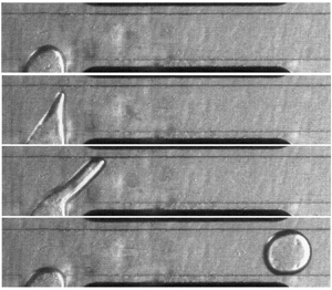
  $1/10$ and 1. Figures 2(a) and 2(b) show the sequential steps involved during droplet generation in a T-shaped microfluidic device for
  $Ca = 1.5 \times 10^{-3}$ (i–vii) and
  $Ca = 3 \times 10^{-3}$ (viii–xiv). In our experiments
  $Ca = 1.5 \times 10^{-3}$ and
  $Ca = 3 \times 10^{-3}$ correspond to a flow rate of continuous phase
  $Q_c=20$ and
  $40\ {\mathrm {\mu }}$L min
 $^{-1}$, respectively. For these low values of capillary number the droplet formation process can be split into four different stages: (i) filling, (ii) squeezing, (iii) breakup and (iv) retraction (Garstecki et al. Reference Garstecki, Fuerstman, Stone and Whitesides2006; Glawdel, Elbuken & Ren Reference Glawdel, Elbuken and Ren2012). As the dispersed phase enters into the main channel during the filling stage, hydrodynamic forces acting on the liquid–liquid interface push the dispersed phase towards the downstream direction resulting in the formation of a characteristic shape, shown in figures 2(iii) and 2(x). In the squeezing stage, the dispersed phase continues to move along the downstream direction, resulting in the elongation of the emerging dispersed phase. Simultaneously, blockage of the flow of continuous phase in the main channel by the dispersed phase results in a build-up of pressure, which squeezes the liquid–liquid interface towards the channel junction. This results in neck formation near the T-junction, as shown in figures 2(
 $v$) and 2(xii). Here the term neck formation implies the narrowing of the thin layer of dispersed phase near the channel junction in such a way that the liquid–liquid interface changes its shape from convex to concave, prior to the breakup of the interface. Further penetration of the dispersed phase into the main channel eventually leads to formation of a droplet (figures 2vi and 2xiii) and retraction of the dispersed phase into the side channel (figures 2vii and 2xiv).

Figure 2. Sequence of droplet formation process for (a)  $Ca = 1.5 \times 10^{-3}$ and (b)
  $Ca = 3 \times 10^{-3}$ at
  $Ca_{E}=0$. The flow rate ratio is
  $Q_{r} = Q_{d}/Q_{c} = 1/10$. (a)
  $Ca = 1.5\times 10^{-3}$ and (b)
  $Ca = 3\times 10^{-3}$.
The droplet lengths  $L$ as a function of flow rate ratio (
 $Q_{r}$) and capillary number (
 $Ca$) in the absence of electric field are presented in figure 3(a). The droplet length is non-dimensionalized with the channel width
  $w$. The shape and size of droplets obtained for different values of
  $Q_{r}$ at
  $Ca = 1.5 \times 10^{-3}$ are shown in figure 3(b). Similar to the experimental observations of Garstecki et al. (Reference Garstecki, Fuerstman, Stone and Whitesides2006) and numerical predictions of De Menech et al. (Reference De Menech, Garstecki, Jousse and Stone2008) and Gupta & Kumar (Reference Gupta and Kumar2010a), the droplet length in our experiments increases linearly with an increase in
  $Q_{r}$ (with
  $Ca$ being constant). A similar variation in the droplet length is observed for
  $Ca = 3 \times 10^{-3}$. These trends are in excellent agreement with the literature (Garstecki et al. Reference Garstecki, Fuerstman, Stone and Whitesides2006; Christopher et al. Reference Christopher, Noharuddin, Taylor and Anna2008).

Figure 3. Variation of droplet length with flow rate ratio for a fixed  $Ca$ in the absence of an electric field. (a) Non-dimensional droplet length (
 $L/w$) as a function of flow rate ratio
  $Q_{r} (= Q_{d}/Q_{c}$) for two different capillary numbers
  $Ca = 1.5 \times 10^{-3}$ and
  $3 \times 10^{-3}$. The droplet length increases linearly with an increase in
  $Q_{r}$ for a fixed
  $Ca$. (b) Corresponding micrographs of the obtained droplets for
  $Ca = 1.5 \times 10^{-3}$.
3.2. Droplet formation with electric field
The effect of an applied electric field on droplet formation was investigated by performing experiments for the same values of  $Ca$ (
 $1.5 \times 10^{-3}$ and
  $3.0 \times 10^{-3}$) and
  $Q_{r}$ (
 ${=}1/10$ to
  $1$) with
  $0\leq Ca_{E}\leq 1$. In our experiments,
  $Ca_E=1$ corresponds to a potential difference of 1300 V between the electrodes. Figure 4(a–c) shows typical stages in the formation of a droplet under the influence of an electric field for
  $Ca_{E}=0.025$, 0.41 and 0.91 at
  $Ca = 1.5\times 10^{-3}$ and
  $Q_{r}=1/10$. Similar to the droplet generation process at
  $Ca_{E}=0$, the first stage involves filling and penetration of the dispersed phase in the main channel. The induced electric stress deforms the penetrating liquid–liquid interface towards the higher potential electrode. This is expected since the electric stress acting on the interface is known to induce the dispersed phase fluid along the direction of the applied electric field for
  $R>S$ (Taylor Reference Taylor1966; Saville Reference Saville1997). On the other hand, the hydrodynamic stress pushes the emerging dispersed phase along the downstream direction. Clearly, the resulting shape of the penetrating dispersed phase at the end of the filling stage is governed by the cumulative effect of electric and hydrodynamic stresses.

Figure 4. Sequence of steps involved in droplet formation process in a T-shaped microfluidic device in the presence of an electric field. (a) The snapshots from (i) to (iii) indicates the general behaviour of the dispersed phase for  $Ca_{E}=0.025$ is similar to
  $Ca_{E}=0$ during the filling stage. A deviation from this behaviour is observed in the end of filling stage (iii) and in the squeezing stage (iv,v) where the dispersed phase is pinned with the top electrode. (b,c) The dispersed phase evolves into a conical shape with an increase in
  $Ca_{E}$ and pins with channel wall near the top electrode. The dispersed phase transforms into a conical shape and becomes reminiscent of the Taylor cone at
  $Ca_{E}=0.91$ (xvi) prior to pinning with the channel wall. A visual inspection of snapshots (vii, xiv, xxi) highlights that the droplet size decreases with an increase in
  $Ca_{E}$. (a)
  $Ca_E = 0.025$; (b)
  $Ca_E = 0.41$; and (c)
  $Ca_E = 0.91$.
The general behaviour of the dispersed phase at  $Ca_{E}=0.025$ during the initial filling stage is observed to be similar to
  $Ca_{E}=0$. However, a deviation is observed near the end of filling stage where the dispersed phase gets pinned to the channel wall (see figure 4iii). The term pinning in the present context refers to the tendency of electric stress to constrain the interface separating continuous and dispersed phases near the top wall, while retaining a thin layer of continuous phase at the wall. The liquid–liquid interface remains pinned with the channel walls near the top electrode as the dispersed phase continues to flow in the downstream direction. Concurrently, the interplay of hydrodynamic and electric stresses acting on the upstream interface lead to the formation of a neck near the channel junction which eventually results in the formation of a droplet.
A significant change in the shape of liquid–liquid interface during the filling stage is observed at higher values of  $Ca_{E}$. For
  $Ca_{E}=0.41$, the emerging interface is strongly pulled towards the top electrode, resulting in the formation of a conical shape with its tip pinned with the channel wall (see figures 4ix and 4x). A comparison of figures 4(iii) and 4(x) highlight that the position where the liquid–liquid interface pins with the channel walls moves upstream with an increase in
  $Ca_{E}$. This indicates that the tendency of the liquid–liquid interface to pin at the channel wall becomes more prominent with an increase in
  $Ca_{E}$. Further, the angle of the conical tip decreases as
  $Ca_{E}$ increases and the interface becomes reminiscent of the Taylor cone (De La Mora & Loscertales Reference De La Mora and Loscertales1994) at
  $Ca_{E}=0.91$ (see figure 4xvi) a few instants prior to pinning with the channel wall. After the pinning, the dispersed phase moves in the downstream direction with the interface pinned only with the top channel wall and a neck is formed near the channel junction. A visual comparison of droplets formed at
  $Ca_{E}=0.025$, 0.41 and 0.91 (see figures 4vii, 4xiv and 4xxi) reveals that the droplet size decreases with an increase in
  $Ca_{E}$ while keeping the flow rates of dispersed and continuous phases unchanged.
Next, the effect of varying flow rate ratio ( $Q_{r}$) and capillary number (
 $Ca$) on the droplet formation process in the presence of applied electric field is discussed. Figure 5 shows the sequential snapshots of droplet formation process for
  $Q_{r}=1/4$ and 3/4 at (panel a)
  $Ca_{E}=0.025$ and (panel b)
  $Ca_{E}=0.41$, respectively. The various stages of the droplet formation process for
  $Q_{r}=1/4$ and 3/4 are observed to be similar to those for
  $Q_{r}=1/10$, shown in figures 4(a) and 4(b). For instance, pinning of the interface with channel walls for
  $Q_{r}=1/4$ and 3/4 occurs at
  $Ca_{E}=0.025$ and is qualitatively similar to that for
  $Q_{r}=1/10$. Likewise, the transformation of the penetrating liquid–liquid interface into a conical shape for
  $Q_{r}=1/4$ and
  $Q_{r}=3/4$ occurs at
  $Ca_{E}=0.41$. Although, the physical mechanism of droplet generation does not change with the flow rate ratio (
 $Q_r$), the droplet length increases with an increase in
  $Q_r$.

Figure 5. Images of droplet formation process for (a)  $Ca_{E}=0.025$ and (b) 0.41 at
  $Ca = 1.5 \times 10^{-3}$, and
  $Q_{r}=1/4$ (i–viii) and
  $3/4$ (ix–xvi). For each
  $Q_{r}$, the sequence of steps involved in the droplet formation process are similar to
  $Q_{r}=1/10$ under the influence of an electric field.
Figure 6 shows a comparison of the droplet formation process for (panel a)  $Ca=1.5 \times 10^{-3}$ and (panel b)
  $Ca = 3 \times 10^{-3}$ at
  $Ca_{E}=0.025$ and
  $Q_{r}=1/10$. Although the droplet formation process appears similar, the pinning behaviour of the liquid–liquid interface varies as
  $Ca$ is increased from
  $1.5 \times 10^{-3}$ to
  $3 \times 10^{-3}$. For
  $Ca = 1.5 \times 10^{-3}$, the interface pins with the channel walls while moving downstream, whereas no pinning is observed for
  $Ca=3 \times 10^{-3}$. The pinning of the interface with the channel walls near the top electrode is governed by the cumulative effect of the electric and viscous stresses acting on the liquid–liquid interface. The electric stress pulls the dispersed phase towards the top electrode while the viscous stress exerted by the continuous phase (flowing through the gap between the dispersed phase and channel walls) deforms the dispersed phase in the flow direction. Therefore, the pinning occurs in the regime where the electric stress dominates the viscous stress. The fact that pinning occurs for
  $Ca = 1.5 \times 10^{-3}$ and not for
  $Ca = 3 \times 10^{-3}$ (as shown in figures 6iv and 6vii) highlights that viscous stress exerted by the continuous phase for the latter case becomes comparable with the electric stress at
  $Ca_{E}=0.025$, thereby inhibiting the pinning of the interface with the channel wall. Further, the outcomes presented in figures 5 and 6 clearly suggest that the pinning of liquid–liquid interface is a strong function of
  $Ca$ and is independent of
  $Q_{r}$.

Figure 6. Comparison of droplet formation process for  $Ca = 1.5 \times 10^{-3}$ and
  $3 \times 10^{-3}$ at
  $Q_{r}=1/10$ and
  $Ca_{E}=0.025$. The sequence of steps involved in the droplet formation process for both
  $Ca$ are similar except that the dispersed phase pins with the channel walls while propagating towards the downstream direction, whereas no pinning is obtained at
  $Ca = 3 \times 10^{-3}$. (a)
  $Ca = 1.5 \times 10^{-3}$ and (b)
  $Ca = 3 \times 10^{-3}$.
To quantify the effect of  $Ca$,
$Ca$,  $Q_{r}$ and
  $Ca_{E}$ on the droplet length
  $L$, the variation of non-dimensional droplet length
  $(L/w)$ for various
  $Ca_{E}$ and
  $Q_{r}$ at
  $Ca = 1.5 \times 10^{-3}$ and
  $3 \times 10^{-3}$ is presented in figure 7. The symbols denote the experimental measurements and the dashed lines represent the empirical correlation (discussed later in § 3.3). Figures 7(a) and 7(b) show a continuous decrease in the droplet length with increasing
  $Ca_{E}$ for fixed
  $Q_{r}$ at
  $Ca = 1.5 \times 10^{-3}$ and
  $3 \times 10^{-3}$, respectively. Similar qualitative variation for droplet length with
  $Ca_{E}$ was observed for all other
  $Q_r$. The variation of droplet length with
  $Q_{r}$ at a fixed value of
  $Ca_{E}$ for
  $Ca=1.5 \times 10^{-3}$ and
  $3\times 10^{-3}$ is shown in figures 7(c) and 7(d), respectively. The droplet length increases linearly with
  $Q_{r}$ for all values of
  $Ca_{E}$.

Figure 7. Variation of droplet length as a function of  $Ca_{E}$ and
  $Q_{r}$ for a particular
  $Ca$. In panels (a,b) for a fixed value of
  $Ca$ and
  $Q_{r}$, the droplet length decreases with increase in
  $Ca_{E}$. Panels (c,d) illustrate that keeping
  $Ca$ and
  $Ca_{E}$ fixed, the droplet size increases with increase in
  $Q_{r}$. (e) Polydispersity obtained in the droplet size distribution is reported for
  $Ca_{E} = 0$, 0.23 and 0.91 in terms of PI. Since
  $\textrm {PI} < 5\,\%$, the droplets obtained for a particular
  $Ca$,
$Ca$,  $Q_{r}$ and
  $Ca_{E}$ are highly monodisperse. (a)
  $Ca= 1.5 \times 10^{-3}$; (b)
  $Ca= 1.5 \times 10^{-3}$; (c)
  $Ca = 3 \times 10^{-3}$; (d)
  $Ca = 3 \times 10^{-3}$ and (e)
  $Ca = 1.5 \times 10^{-3}$.
The data presented in figure 7 shows that applying an electric field enables formation of emulsions that are otherwise not possible to create by controlling  $Q_r$ and
  $Ca$. For example, to generate an emulsion with high volume fraction of the dispersed phase requires a higher value of
  $Q_r$. Generating droplets at high
  $Q_r$, however, increases the droplet size as shown in figures 7(c) and 7(d). The experimental data presented in figures 7(a) and 7(b) proves that an electric field can be used to reduce the droplet size without changing
  $Q_r$, i.e. while keeping the volume fraction of the emulsion fixed. Moreover, application of an electric field does not affect the monodispersity of droplets. To show this, the droplet size distributions for three different values of
  $Ca_{E}$ are presented for
  $Q_{r} = 1/10$ and
  $Ca = 1.5 \times 10^{-3}$ in figure 7(e). The droplet size distribution remains narrow for the various
  $Ca_{E}$ considered herein. Alternatively, the heterogeneity in the size of droplets can be quantified in terms of the polydispersity index (PI), which is defined as
 \begin{equation} \textrm{PI} = \frac{\zeta}{L}\times 100\,\%, \end{equation}
where  $\zeta$ is the sample standard deviation of the measured droplet lengths. As shown in figure 7(e), the PI is less than
  $5\,$% for all values of
  $Ca_{E}$ which shows that monodisperse droplets are generated even in the presence of an electric field.
3.3. Functional relationship
The dimensional analysis presented in § 2.3 and the experimental data presented in figure 7 suggests that the non-dimensional droplet length  $L/w$ depends only on
  $Ca$,
$Ca$,  $Ca_{E}$ and
  $Q_{r}$ for the chosen continuous and dispersed phases; mathematically that is
 \begin{equation} \frac{L}{w} = f(Ca, Ca_{E}, Q_{r}).\end{equation}
This functional relationship can be brought out using the experimental data. Further, it is essential that the dependence of  $L/w$ on
  $Ca$,
$Ca$,  $Ca_{E}$ and
  $Q_{r}$ captures the essential physics of droplet formation when reconciled with published work. In this regard, in the limit
  $Ca_E\approx 0$, (3.2) must reduce to the relationship proposed by Garstecki et al. (Reference Garstecki, Fuerstman, Stone and Whitesides2006) for droplet length in a T-junction microchannel. It is worth noting that Garstecki et al. (Reference Garstecki, Fuerstman, Stone and Whitesides2006) modelled the droplet length as a linear combination of the distance that the dispersed phase enters into the main channel during the filling (
 $L_{{fill}}$) and the squeezing stages (
 $L_{{squeeze}}$); that is
 \begin{equation} L=L_{{fill}}+L_{{squeeze}}.\end{equation}
Garstecki et al. (Reference Garstecki, Fuerstman, Stone and Whitesides2006) showed that  $L_{{fill}}$ is proportional to the channel width, i.e.
  $L_{{fill}} = \alpha _{1}w$, where
  $\alpha _{1}$ is a proportionality constant. Further, in this model
  $L_{{squeeze}}$ depends upon the rate at which the dispersed phase enters in the main channel during the squeezing stage and the time taken by the continuous phase to squeeze the neck formed near the channel junction, i.e.
  $L_{{squeeze}} = du_{d}/u_{c} = dQ_{d}/Q_{c}$. Here
  $d$ is a characteristic width which further depends upon the radius of curvature
  $R_{c}$ of the neck. It was shown (Garstecki et al. Reference Garstecki, Fuerstman, Stone and Whitesides2006) the dimensionless droplet length for
  $Ca_{E}=0$ can be expressed as
 \begin{equation} \frac{L}{w}=\alpha_{1}+\beta_{1}Q_r, \end{equation}
where  $\beta _{1}=R_{{c}/w}$ is a parameter that can be obtained by fitting experimental data. Because the droplet size in the absence of electric field (
 $Ca_{E}=0$) is governed only by
  $Ca$ and
  $Q_{r}$ (from (3.2)), it can inferred that
  $\alpha _{1}$ and
  $\beta _{1}$ are functions of
  $Ca$. It should be emphasized that the validity of (3.4) has been shown by various experimental (Christopher et al. Reference Christopher, Noharuddin, Taylor and Anna2008) and numerical studies (De Menech et al. Reference De Menech, Garstecki, Jousse and Stone2008; Gupta & Kumar Reference Gupta and Kumar2010a) on droplet generation in T-junction microchannels.
Because the two stages of droplet formation, namely filling and squeezing, do not change with the application of an electric field, the dimensionless droplet length in an electrified T-junction can also be expressed as
 \begin{equation} \frac{L}{w}=\alpha_{1}^{'}+\beta_{1}^{'}Q_{r}.\end{equation}
Such a linear relationship between droplet length and flow rate ratio  $Q_r$ is also supported by the experimental data presented in figures 7(c) and 7(d). In (3.5),
  $\alpha _{1}^{'}$ and
  $\beta _{1}^{'}Q_{r}$ represent the non-dimensional lengths of the dispersed phase that enters in the main channel during the filling and squeezing stages, respectively.
The experimentally measured position of the liquid–liquid interface during filling and squeezing stages is shown in figures 8(a) and 8(b) to understand the dependence of these lengths on the electric field. As shown in figure 8(a), the length of dispersed phase penetrating into the main channel during the filling stage decreases with an increase in  $Ca_{E}$. This suggests that
  $\alpha _{1}^{'}$ depends on
  $Ca_E$, in addition to its dependence on
  $Ca$. Because
  $\alpha _{1}^{'}$ is a decreasing function of
  $Ca_E$ and it must reduce to
  $\alpha$ in the limit of
  $Ca_E=0$,
 \begin{equation} \alpha_{1}^{'}=\alpha_{1}(Ca)-g_{1}(Ca, Ca_{E}),\end{equation}
where  $g_{1}(Ca, Ca_{E}=0)=0$. Figure 8(b) shows that the radius of curvature of the neck increases with an increase in
  $Ca_{E}$ which indicates
  $\beta _{1}^{'}$ is also governed by
  $Ca_{E}$ other than
  $Ca$. Because
  $R_{c}$ increases with
  $Ca_{E}$ and
  $\beta _{1}^{'}$ must reduce to
  $\beta _{1}$ for
  $Ca_{E}=0$,
  $\beta _{1}^{'}$ can be expressed as
 \begin{equation} \beta_{1}^{'}=\beta_{1}(Ca)+g_{2}(Ca, Ca_{E}),\end{equation}
where  $g_{2}(Ca, Ca_{E}=0)=0$. For a fixed capillary number, our experimental data suggests that
  $g_1$ and
  $g_2$ scale with electric capillary number as
  $\sim Ca_E^{0.5}$. Therefore, we express the length of the droplet formed in the presence of electric field as
 \begin{equation} \frac{L}{w}=\left(\alpha_{1}-\alpha_{2}Ca_{E}^{0.5}\right)+ \left(\beta_{1}+\beta_{2}Ca_{E}^{0.5}\right)Q_{r}.\end{equation}
Here,  $\alpha _{1}$,
  $\alpha _{2}$,
  $\beta _{1}$ and
  $\beta _{2}$ are empirical constants which depend only on the capillary number.

Figure 8. Outline of the dispersed phase interface entering in the main channel for different values of  $Ca_{E}$. Panel (a) shows that the length of the dispersed phase entered in the main channel is a function of
  $Ca_{E}$ and decreases with an increase in
  $Ca_{E}$. Panel (b) illustrates that the curvature radius at the upstream end of the dispersed phase varies with
  $Ca_{E}$. Here
  $R_{c}$ and
  $R_{c}^{'}$ are the neck radius for
  $Ca_{E} = 0$ and 0.23, respectively. Panels (c,d) show a comparison of the non-dimensional droplet length obtained from the experiments performed and proposed correlation for different values of
  $Ca$. (a) Filling stage and (b) squeezing stage.
Equation (3.8) was used to perform regression on the experimentally measured droplet lengths corresponding to  $Ca=1.5\times 10^{-3}$ and
  $3.0 \times 10^{-3}$. The droplet lengths predicted by the empirical correlation
  $(L/w)_{{corr}}$ are in excellent agreement with the experimental data
  $(L/w)_{{exp}}$ as shown in figures 8(c) and 8(d). The values of the empirical constants are also provided in figures 8(c) and 8(d). The deviation between the experiments and correlation predictions is reported in terms of the mean square error (MSE) and is shown in figures 8(c) and 8(d) for
  $Ca = 1.5 \times 10^{-3}$ and
  $3 \times 10^{-3}$. The MSE is calculated as
 \begin{equation} \textrm{MSE} = \frac{1}{w}\sqrt{\frac{\sum_{i}{\left(L_{{exp,i}}-L_{{corr,i}}\right)^{2}}}{n}}. \end{equation}
The MSE obtained for  $Ca = 1.5 \times 10^{-3}$ and
  $3 \times 10^{-3}$ is found to be less than 0.1 %. This further highlights that the proposed correlation can provide an accurate estimate of droplet length formed for different values of
  $Ca_{E}$ and
  $Q_{r}$ for
  $Ca = 1.5 \times 10^{-3}$ and
  $3 \times 10^{-3}$.
3.4. Mechanism of droplet formation
Although the experiments reported in the previous section demonstrate the droplet formation process, they do not provide a complete understanding of the reasons leading to a decrease in droplet size in an electrified T-junction device. Numerical simulations, on the other hand, provide a convenient alternative to interrogate all dynamic variables of a system. Consequently, we undertake a numerical investigation in this section to elucidate the underlying mechanism of the droplet formation process. The simulations have been performed by coupling the electrostatics for leaky dielectric fluids with the hydrodynamics in the framework of the lattice Boltzmann method (LBM). A brief background of the method is given in appendix A and the details can be obtained from previous publications (Singh et al. Reference Singh, Bahga and Gupta2019a,Reference Singh, Bahga and Guptab).
A schematic illustration of the computational domain along with the boundary conditions used to simulate the droplet formation process under the influence of an electric field is shown in figure 9. The computational domain consists of a T-junction microchannel with two orthogonal inlets and a single outlet. The continuous phase flows in the main channel, while the dispersed phase enters from the side channel. The channels are rectangular in cross-section with an aspect ratio  $h/w = 0.6$, where
  $w$ and
  $h$ denote the width and height of the microchannel, respectively. The continuous and dispersed phases are considered to be immiscible and flow into the respective microchannels with flow rates
  $Q_{c}$ and
  $Q_{d}$, respectively. Therefore, a constant mass flux is specified at the inlet and outlet at each time instant (Gupta & Kumar Reference Gupta and Kumar2010a). Further, a constant pressure is maintained at the outlet of the microchannel. The dispersed phase is considered to be non-wetting while the continuous phase is assumed to wet the channel walls. The fluid nodes near the channel walls are considered to be separated from the solid nodes by half a lattice unit and second-order bounce-back scheme is used to apply no-slip boundary condition (Krüger et al. Reference Krüger, Kusumaatmaja, Kuzmin, Shardt, Silva and Viggen2017).

Figure 9. Schematic of the T-junction microchannel used for simulating the droplet formation process under the influence of an electric field. The channels have rectangular cross-section having an aspect ratio  $h/w = 0.6$. Part of the channel walls at a distance
  $\xi$ from the channel junction in the downstream direction are considered as electrodes. These electrodes are considered as rectangular sheets with width
  $w_{1}$ and height
  $h$. An electric field along the transverse direction of the flow is applied by imposing an electric potential
  $U = U_{o}$ at the top electrode, while the bottom is grounded. The remaining channel walls are considered to be electrically insulating.
Parts of the channel walls at a distance  $\xi$ from the channel junction, as shown in figure 9, are modelled as electrodes. The electrodes are considered as rectangular sheets with width
  $w_{1}$ and height
  $h$. Unlike in experiments, a layer of dielectric material between the electrode and fluids has been ignored. Initially, the electric potential and the free charge distribution in the fluids are assumed to be zero. At
  $t=0$, an electric field is applied by imposing an electric potential
  $U = U_{o}$ at the top electrode, while the bottom electrode is grounded. The remaining channel walls are considered to be electrically insulating, that is,
  $\boldsymbol {n} \boldsymbol{\cdot} \boldsymbol {E}=0$, where
  $\boldsymbol {n}$ is a unit vector normal to the channel walls.
Before discussing the mechanism, the capability of the employed multicomponent model is established by comparing simulation predictions with experimental measurements. To this end, droplet formation process in a T-junction microchannel is simulated on a computational domain of size 351 ${\rm \Delta} x \times 60{\rm \Delta} y \times 36{\rm \Delta} z$. The hydrodynamic properties of fluids are considered to be
  $\rho _{r} = \rho _{d}/\rho _{c} = 1$ and
  $\lambda = \mu _{d} /\mu _{c} = 1/25$. The LBM parameters used to perform the simulation are defined in table 2. These parameters are obtained by using dimensional analysis to relate the length, mass, time and electric potential in physical units to LBM units. The physical constant used for the conversion are density, interfacial tension, channel width and voltage difference. This gives the dimensional scaling factors as length
  $C_{L} = 8.33 \times 10^{-6}$ m,
  $C_{T} = 1.23 \times 10^{-6}$ s, mass
  $C_{M} = 5.79 \times 10^{-13}$ kg and voltage
  $C_{V} = 50$ V. Figure 10 shows snapshots of droplet formation process at
  $Ca_{E} = 0$ obtained from our (panel a) numerical simulations and (panel b) experiments for
  $Ca = 3\times 10^{-3}$ and
  $Q_{r}=1/10$. The comparison shows that results obtained from numerical simulations for
  $Ca_{E} = 0$ are consistent with experimental observations.
Table 2. The LBM values corresponding to the physical parameters used to perform simulations.


Figure 10. Comparison of droplet formation process obtained from (a) numerical simulations and (b) experiments at  $Ca = 3 \times 10^{-3}$,
  $Q_{r}=1/10$ and
  $Ca_{E}=0$.
Next, a comparison of simulations and experiments of droplet formation process in the presence of an electric field is presented. The electrical properties of fluids used in the experiments are such that the conductivity ratio  $R \sim 10^{6}$ and the permittivity ratio
  $S=28.6$ (see table 1). The numerical model used in the present work suffers from numerical instabilities for fluids having large contrast in electrical properties. Hence, the values of both conductivity and permittivity ratio in the simulations are taken to be
  $R = S = 10$. Other numerical models (Collins et al. Reference Collins, Jones, Harris and Basaran2008; Paknemat, Pishevar & Pournaderi Reference Paknemat, Pishevar and Pournaderi2012) have demonstrated the capability to handle the large gradients in electrical properties of fluids across the fluid–fluid interface. Although the values of
  $R$ and
  $S$ differ significantly from the electrical properties of the liquids used in the experiments, the electrohydrodynamic behaviour of both the systems is similar. This can be justified by considering the case of an immiscible droplet suspended in another liquid and subjected to an electric field. The normal and tangential electric stress acting on the interface of the droplet are given as (Taylor Reference Taylor1966)
 \begin{equation} \boldsymbol{F}_{E,r}=\frac{9E_{o}^{2}\varepsilon_{c}}{8{\rm \pi} (2+R)^{2}} \left[S-1+\lbrace(R^{2}+1-2S) \rbrace \cos^{2}\theta \right] \end{equation}
and
 \begin{equation} \boldsymbol{F}_{E,\theta} = \frac{-9E_{o}^{2}\varepsilon_{c}}{4{\rm \pi} (2+R)^{2}}(R-S)\cos\theta \sin\theta, \end{equation}
respectively. Here  $E_{\circ }$ is the magnitude of applied electric field and subscript
  $c$ denotes outer liquid. Equation (3.11) clearly indicates that the tangential electric stress
  $(\boldsymbol {F}_{E,\theta })$ is negligible for liquids with
  $R \gg 1$ and the electrohydrodynamics is governed solely by the normal electric stress
  $(\boldsymbol {F}_{E,r})$. The same condition can also be arrived at for liquids with
  $R=S$. Moreover, (3.10) suggests that the magnitude of normal stress for liquids having
  $R \sim 10^6$ and
  $S=28.6$ used in the experiments can be similar to the liquids used in simulations having
  $R=10$ and
  $S=10$. This is because, for
  $R = 10$ and above, the magnitude of the normal stress on the dispersed phase approaches the asymptotic limit of
  $R \gg 1$.
Figure 11 demonstrates a comparison of droplet formation process under the influence of an electric field obtained from (panel a) numerical simulations and (panel b) experiments at  $Ca = 3 \times 10^{-3}$,
  $Q_{r}=1/10$ and
  $Ca_{E}=0.23$. As shown in figure 11(a), the dispersed phase initially penetrates in the main channel and obstructs the flow of the continuous phase. The dispersed phase transforms into a conical shape as it approaches the top electrode, eventually pinning at the channel walls (figure 11ii). After pinning, the dispersed phase further moves in the main channel with the interface pinned with the top wall and the process culminates with the generation of a droplet in the main channel. Even though the electrical properties of fluids taken in simulations are different when compared with experiments, a comparison of figures 11(a) and 11(b) shows that the numerical model qualitatively captures all aspects of droplet formation process exhibited in experiments in the presence of an electric field.

Figure 11. Images demonstrating comparison of droplet formation process in the presence of an electric field obtained from (a) numerical simulations and (b) experiments at  $Ca = 3 \times 10^{-3}, Q_{r}=1/10$ and
  $Ca_{E}=0.23$.
As compared to  $Ca_{E}=0$, the following notable differences in the droplet formation process are obtained in our experiments with the inclusion of electric field: (i) the dispersed phase transforms into a conical shape while penetrating in to the main channel; (ii) it extends and pins with the channel wall; and (iii) a droplet of smaller size is formed in the presence of the electric field for the same physical and flow parameters. The variation in shape and pinning of the dispersed phase using the mathematical model is elucidated by examining the distribution of electric potential in the channel. Figure 12(a) shows the shape of the dispersed phase as it enters in the main channel and figure 12(b) shows the corresponding distribution of electric potential in the fluid domain in the plane passing through the middle of the channel along the
  $xy$ direction. As shown in figures 12(i) and 12(ii), the dispersed phase initially penetrates in the main channel and obstructs the flow of the continuous phase. This leads to a non-uniform distribution of electric field in the fluids, having the maximum value near the tip of the dispersed phase as indicated by the proximity of equipotential lines in figures 12(iv) and 12(
 $v$). Consequently, a non-uniform electric stress gets induced on the interface which tends to deform the dispersed phase along the direction of electric field (which is consistent with the theoretical predictions of
Taylor (Reference Taylor1966)). The cumulative action of the hydrodynamic and electric stress further stretches the dispersed phase towards the top electrode and results in the transformation of the interface into a conical shape, as shown in figures 12(iii) and 12(vii). As shown in figure 12(iii), the tip of the three-dimensional cone is formed near the channel walls. Subsequently, further inflow of the dispersed phase leads to the pinning and sliding of the interface along with the channel walls as shown in figures 12(iv) and 12(viii).
$v$). Consequently, a non-uniform electric stress gets induced on the interface which tends to deform the dispersed phase along the direction of electric field (which is consistent with the theoretical predictions of
Taylor (Reference Taylor1966)). The cumulative action of the hydrodynamic and electric stress further stretches the dispersed phase towards the top electrode and results in the transformation of the interface into a conical shape, as shown in figures 12(iii) and 12(vii). As shown in figure 12(iii), the tip of the three-dimensional cone is formed near the channel walls. Subsequently, further inflow of the dispersed phase leads to the pinning and sliding of the interface along with the channel walls as shown in figures 12(iv) and 12(viii).

Figure 12. Transformation of the dispersed phase shape while entering in the main channel and evolution of equipotential lines in fluids at  $Ca_{E}=0.23$. The potential difference between the successive equipotential lines is 0.421. The equipotential lines redistribute in the fluids as the dispersed phase penetrates in the main channel. The electric field and induced electric stress are maximum near the dispersed phase tip.
The reduction in droplet size with an increase in  $Ca_{E}$ occurs due to the build-up of electric field strength near the upstream interface (as shown in figures 12vii and 12viii) and can be explained by comparing the time evolution of the dispersed phase for
  $Ca_{E}=0$ and 0.23 as shown in figure 13. While the shape of dispersed phase is similar for
  $Ca_{E}=0$ and
  $Ca_{E}=0.23$ till
  $t^{*}=13.74$ (figure 13a), a considerable change is observed at later stages. For
  $Ca_{E}=0$, the dispersed phase continues to enter in the main channel and blocks the flow of the continuous phase. For
  $Ca_{E}=0.23$, on the other hand, the dispersed phase pins with the channel walls and forms a neck near the channel junction as it propagates in the main channel as shown in figure 13(b–d). This early neck formation occurs due to the tendency of the electric stress to deform the interface along the direction of the electric field, thereby leading to a decrease in the distance between the upstream interface and the channel edge. Since the strength of induced electric stress is proportional to the applied electric field, the time required for neck formation decreases with an increase in
  $Ca_{E}$. Consequently, the droplet size decreases with an increase in
  $Ca_{E}$.

Figure 13. A comparison of dispersed phase profile while penetrating in the main channel for  $Ca_{E} = 0$ and
  $Ca_{E}=0.23$ at different time instances. Here
  $t^{*}=tu_{c}/h$ is the non-dimensional time. The dispersed phase interface at
  $Ca_{E}=0$ and
  $Ca_{E}=0.23$ are represented by dashed and solid lines, respectively. The time required for the formation of a neck in the dispersed phase decreases with the application of an electric field, thereby leading to a reduction in the droplet size.
  $(a) \ t^{*} = 13.74; (b) \ t^{*} = 15.68; (c) \ t^{*} = 15.90 \ {\rm and} \ (d) \ t^{*} = 16.76.$
Apart from understanding the mechanism of the droplet formation process, the effect of including electric field on the dynamics of the droplet formation is also investigated. This is elucidated by comparing the evolution of pressure build-up at a point P upstream of the junction shown in figure 13(a) (De Menech et al. Reference De Menech, Garstecki, Jousse and Stone2008; Sivasamy et al. Reference Sivasamy, Wong, Nguyen and Kao2011) for  $Ca_{E} = 0$, 0.125 and 0.23 at
  $Ca = 3 \times 10^{-3}$ and
  $Q_{r}=1/10$, and as is shown in figure 14. Here
  $p^{*}=p/(\rho u_{c}^{2})$ is the non-dimensional pressure. The inset images show the position of the dispersed phase in the main channel during various stages of droplet formation at different time instants for
  $Ca_{E}=0$ (a–c) and 0.23 (d–f). For
  $Ca_{E}=0$, the pressure can be observed to rise gradually owing to the blockage of the available area for the flow of continuous phase with time (inset image (a)). As the pressure reaches a maximum value (inset image (b)), the continuous phase begins to squeeze the neck towards the edge of the T-junction (inset image (c)). Beyond this point, the developed pressure decreases and a sudden drop in the pressure is observed with the clearing of passage for flow of continuous phase and formation of a droplet in the main channel.

Figure 14. Pressure build-up in the continuous phase upstream of the T-junction with the evolution of dispersed phase in main channel at different values of  $Ca_{E}$. Here
  $p^{*}=p/(\rho u_{c}^{2})$ is the non-dimensional pressure and
  $t^{*}=tu_{c}/h$ is the non-dimensional time. The solid line represents evolution of pressure for
  $Ca_{E}=0$, while the dashed-dot and dashed lines represent
  $Ca_{E}=0.125$ and 0.23, respectively. The pressure is monitored at a point P upstream of the channel junction (see figure 13a). The pressure build-up in the continuous phase decreases with an increase in
  $Ca_{E}$, thereby suggesting that the droplet formation process in the presence of an electric field is predominantly governed by the electric stress induced on the diffused phase interface.
Similar to  $Ca_{E}=0$, the penetration of dispersed phase in the main channel under the influence of an electric field also leads to a pressure build-up in the continuous phase (inset image (d)). This pressure increases continuously and reaches a maximum as the dispersed phase moves near the top electrode (inset image (e)). Beyond this point, the cumulative action of hydrodynamic pressure and electric stress deforms the upstream interface towards the downstream direction. Consequently, the pressure build-up in the continuous phase decreases and drops rapidly until a droplet is formed in the main channel. However, the maximum pressure rise in the continuous phase decreases with an increase in
  $Ca_{E}$, as can be seen from figure 14. The lowering of the peak pressure results due to the electric stress induced on the liquid–liquid interface as the dispersed phase enters in the main channel. The electric stress acting on the interface under the influence of the electric field leads to the interface being pulled towards the top wall in a short duration of time. At the same time, the electric stress also deforms the upstream interface along the direction of flow in the main channel. This leads to a change in the curvature of the upstream interface from convex to concave, thereby speeding up neck formation. The role of the electric field in promoting neck formation is also evident from figures 13(c) and 13(d), where the curvature of the upstream interface (denoted by solid lines) is shown to transform in the presence of the applied electric field. Because the electric field expedites the neck formation, a lower upstream pressure is required to overcome the interfacial force and pinch off a droplet. On the other hand, in the absence of an electric field (
 $Ca_{E}=0$), the neck formation is purely hydrodynamically driven. As shown in figures 13(c) and 13(d), for
  $Ca_{E}=0$ (denoted by dashed lines), there is an insignificant variation in the curvature of the interface when the dispersed phase enters in the main channel. Therefore, in the absence of an electric field, a higher upstream pressure is required for neck formation. Since the strength of induced electric stress increases with
  $Ca_{E}$, the peak value of pressure during the droplet break-up process further decreases with an increase in
  $Ca_{E}$, as shown in figure 14. This decrease in the peak value of pressure required for the droplet formation shows that the droplet formation process is predominantly governed by electric stresses acting on the liquid–liquid interface with an increase in
  $Ca_{E}$.
4. Conclusions
In this paper, a systematic experimental investigation of the droplet formation process under the influence of an electric field in a T-junction microchannel was presented. The experimental analysis involved the fabrication of a T-shaped microfluidic device integrated with two non-contacting electrodes on a PMMA substrate. The reported experiments herein involved scenarios where hydrodynamics is typically governed by the interplay between the squeezing pressure exerted by the continuous fluid and the interfacial tension acting at the liquid–liquid interface. Although the sequential pattern of the droplet formation remained similar to  $Ca_{E}=0$, application of an electric field transformed the mechanism of droplet formation. Under the influence of an electric field, the dispersed phase was pinned with the channel walls near the top electrode while penetrating the main channel. The pinning behaviour of the dispersed phase was observed to be a function of Ca and
  $Ca_{E}$, and independent of the flow-rate ratio of the fluids. A greater pinning tendency is induced with an increase in
  $Ca_{E}$ and decrease in
  $Ca$. Moreover, prior to the pinning with the channel wall, an increase in
  $Ca_{E}$ induced the deformation of the dispersed phase into a conical shape. These variations resulted in a monotonic reduction in the droplet size when
  $Ca$ and
  $Q_{r}$ remain unchanged. Thereby, a significant reduction in the droplet size was obtained which could not have been achieved by the traditional methods of droplet formation. The generated droplets feature high monodispersity with polydispersity index values of less than 5 %. Further, the obtained results were used to formulate an empirical correlation to quantify the dependence of droplet length in terms of
  $Ca_{E}$ and
  $Q_{r}$. The predictions from the correlation were demonstrated to be in good agreement with the experimental measurements.
Numerical simulations were also performed to explain the departure in the droplet formation process and to explain the changes observed in the droplet size formed in the presence of an electric field. The numerical analyses revealed that the electric stress distributes non-uniformly over the fluid–fluid interface as the dispersed phase penetrates the main channel. The non-uniform distribution of electric stress stretched the dispersed phase towards the top electrode, resulting in the deformation of the interface into a conical shape and pinning of the dispersed phase with the channel walls. Moreover, the deformation induced in the interface led to the onset of an early neck formation as compared to  $Ca_{E}=0$. Consequently, droplets formed for the same flow parameters in the presence of an electric field were smaller in size when compared with the droplets formed at
  $Ca_{E}=0$. Furthermore, numerical simulations were used to understand the dynamics of the droplet formation by examining the evolution of the hydrodynamic pressure upstream of the channel junction for different values of
  $Ca_{E}$. The pressure build-up decreased with an increase in
  $Ca_{E}$ thereby implying that the dominating contribution in the dynamics of breakup arises from the electric stress acting at the fluid–fluid interface.
Declaration of interests
The authors report no conflict of interest.
Appendix A
The developed numerical method involves coupling of electrostatic and hydrodynamic models within the framework of the lattice Boltzmann method. In this formulation, the fluids are considered to have equal density and behave as leaky dielectric fluids (Taylor Reference Taylor1966). The immiscible fluids are separated from each other by a diffused interface across which the fluid properties undergo a continuous variation. This is achieved by defining a colour function  $C$ based upon the density of fluids, expressed as
 \begin{equation} C(\boldsymbol{x},t)=\frac{\rho_{c}(\boldsymbol{x},t)-\rho_{d}(\boldsymbol{x},t)}{\rho_{c} (\boldsymbol{x},t)+\rho_{d}(\boldsymbol{x},t)}, \end{equation}
where  $\rho$ denotes density and subscript
  $c$ and
  $d$ represents continuous and dispersed phase, respectively. The value of
  $C$ varies insignificantly in the pure phase and undergoes a smooth transition across the fluid–fluid interface, thereby creating a diffused region separating the two immiscible fluids. The unit normal vector
  $\boldsymbol {n}$ to this diffused interface is obtained using the gradient of the colour function, defined as
 \begin{equation} \boldsymbol{n}=-\frac{\boldsymbol{\nabla} C}{|\boldsymbol{\nabla} C|}. \end{equation}
Using this unit vector, the local curvature  $\kappa$ of the diffused interface is determined, given as
 \begin{equation} \kappa = \frac{1}{R_{c}} = -\boldsymbol{\nabla}_{S}\boldsymbol{\cdot} \boldsymbol{n}, \end{equation}
where  $R_{c}$ is the local radius of curvature of the diffused interface and
  $\boldsymbol {\nabla }_{S}$ is the surface gradient operator. Using the gradient of the colour function and radius of curvature of the interface, the body term due to the interfacial tension
  $\boldsymbol {F}_{\text {I}}$ is calculated, defined as
 \begin{equation} \boldsymbol{F}_{\text{I}}=-\frac{1}{2R_{c}}\gamma \boldsymbol{\nabla} C, \end{equation}
where  $\gamma$ is the interfacial tension. This body force term is further used to calculate the source term, given as (Guo, Zheng & Shi Reference Guo, Zheng and Shi2002)
 \begin{equation} \phi_{I}=w_{i}\left(1-\frac{1}{2\tau} \right)\left[\frac{\boldsymbol{e}_{i}-\boldsymbol{u}}{c_{s}^{2}}+ \frac{(\boldsymbol{e}_{i}\cdot \boldsymbol{u})}{c_{s}^{4}} \right]\cdot \boldsymbol{F}_{I},\end{equation}
which in turn is incorporated in the collision step of the lattice Boltzmann method (Singh et al. Reference Singh, Bahga and Gupta2019b). In the above equation (A 5),  $w_{i}$ is the weight function,
  $\tau$ is the relaxation time,
  $\boldsymbol {u}$ is the velocity vector,
  $\boldsymbol {e}$ is the lattice vector and
  $c_{s}$ is the speed of sound in lattice units.
For the electrostatic part of the framework, the local electrical properties are assumed to vary as
 \begin{equation} \left.\begin{gathered} \varepsilon(\boldsymbol{x},t) = \frac{\varepsilon_{c}(1+C)+\varepsilon_{d}(1-C)}{2}, \\ \sigma(\boldsymbol{x},t)= \frac{\sigma_{c}(1+C)+\sigma_{d}(1-C)}{2}, \end{gathered}\right\} \end{equation}
where  $\varepsilon$ and
  $\sigma$ are the dielectric permittivity and electric conductivity of the fluids. The electric field applied on the system is related to the electrical conductivity and free charge density by the charge conservation equation (Ramos Reference Ramos2011)
 \begin{equation} \frac{\partial \rho_{f}}{\partial t} + \boldsymbol{\nabla} \boldsymbol{\cdot} (\rho_{f}\boldsymbol{u}+\sigma \boldsymbol{E})=0, \end{equation}
where  $\rho _{f}=\boldsymbol {\nabla } \boldsymbol {\cdot } (\varepsilon \boldsymbol {E})$. As the charge relaxation time in electrostatics is small compared with other times, (A 7) reduces to
 \begin{equation} \boldsymbol{\nabla} \boldsymbol{\cdot} (\sigma \boldsymbol{E}) = 0. \end{equation}
As electric field is considered to be irrotational in electrostatics,  $\boldsymbol {E}$ can be expressed as
 \begin{equation} \boldsymbol{E}=-\boldsymbol{\nabla} U, \end{equation}
where  $U$ is the electric potential. The application of electric potential leads to an electric stress at the fluid–fluid interface, which in our developed framework is modelled by incorporating a source term due to electric field in the collision step, defined as
 \begin{equation} \phi_{E} = w_{i}\left(1-\frac{1}{2\tau} \right)\left[\frac{\boldsymbol{e}_{i}-\boldsymbol{u}}{c_{s}^{2}}+ \frac{\boldsymbol{e}_{i}\boldsymbol{\cdot} \boldsymbol{u}}{c_{s}^{4}} \right]\boldsymbol{\cdot}\boldsymbol{F}_{E}. \end{equation}
Here  $\boldsymbol {F}_{E}$ is the body force due to the electric field, given as
 \begin{equation} \boldsymbol{F}_{E} = \boldsymbol{\nabla} \boldsymbol{\cdot} \underline{\boldsymbol{T}}_{E} = \rho_{f} \boldsymbol{E} - \tfrac{1}{2}E^{2}\boldsymbol{\nabla} \varepsilon. \end{equation}


