


1. Introduction
Liquid droplet production by a jet-like momentum source is relevant in industrial and biological processes such as combustion efficiency in liquid fuel engines (Hardalupas, Taylor & Whitelaw Reference Hardalupas, Taylor and Whitelaw1990; Hardalupas & Whitelaw Reference Hardalupas and Whitelaw1993), cost constraints in metal powder production (Ünal Reference Ünal1989) for additive manufacturing and aerosol transport during human exhalations (Abkarian et al. Reference Abkarian, Mendez, Xue, Yang and Stone2020; Balachandar et al. Reference Balachandar, Zaleski, Soldati, Ahmadi and Bourouiba2020). The resulting poly-disperse collection of droplets, or spray, interacts with the turbulence in the jet far field. A unified framework is presented where the initial droplet production mechanisms of an air–water spray are connected with the subsequent dispersion in the jet far field.
Studies of the shear layer in co-axial round jets where a central low-momentum liquid jet (density:  $\rho _\ell$, velocity:
  $U_\ell$) is surrounded by high-momentum gas (
 $\rho _g$,
  $U_g$) jet (see
Lasheras & Hopfinger (Reference Lasheras and Hopfinger2000) and Dumouchel (Reference Dumouchel2008) for extensive reviews) emphasize the role of momentum balance across the liquid–gas interface in determining the nature of atomization. The momentum ratio,
 \begin{equation} M=\rho_g U_g^2/(\rho_\ell U_\ell^2), \end{equation}
is an indicator of the momentum balance that sustains the advection of shear-layer vortices at a velocity  $U_c$ such that
  $U_c/U_\ell \sim M^{1/2}$ (Dimotakis Reference Dimotakis1986). A critical value of the momentum ratio has been observed, of the order of
  $M=50$, where the inner jet's momentum is not sufficient to balance that of the outer jet and a recirculating vortex core is established near the nozzle, which truncates the central jet (Rehab, Villermaux & Hopfinger Reference Rehab, Villermaux and Hopfinger1997; Favre-Marinet, Camano & Sarboch Reference Favre-Marinet, Camano and Sarboch1999; Lasheras & Hopfinger Reference Lasheras and Hopfinger2000). Synchrotron radiography measurements implicate this recirculating vortex in the various break-up regimes beyond the critical momentum ratio in a liquid spray (Machicoane et al. Reference Machicoane, Bothell, Li, Morgan, Heindel, Kastengren and Aliseda2019). These processes are often coupled with large-scale instabilities causing strong lateral excursions of the liquid jet known as ‘flapping’ (Delon, Cartellier & Matas Reference Delon, Cartellier and Matas2018) or ‘dilatational waves’, resulting in clustered break-up of a high-momentum liquid core (Engelbert, Hardalupas & Whitelaw Reference Engelbert, Hardalupas and Whitelaw1995; Kumar & Sahu Reference Kumar and Sahu2020).
Once formed, droplets are advected into the far field of the jet where droplet inertia is the fundamental parameter governing dispersion. These processes are parameterized by the ratio of particle response time  $\tau _p$ and fluid characteristic time scale
  $\tau _f$, known as the Stokes number
 \begin{equation} St={\tau_p}/{\tau_f}. \end{equation}
Much of what is known of droplet dispersion has been studied in the context of monodisperse particle-laden jets (PLJs). Lau & Nathan (Reference Lau and Nathan2014, Reference Lau and Nathan2016) observed that dispersion in the far field of the jet was reduced for increasing  $St$, and linked this effect to the initial conditions. In particular, a competition between the Saffman force (Saffman Reference Saffman1965) tending to accumulate large
  $St$ particles near the centreline and turbophoresis (Reeks Reference Reeks1983) which tends to accumulate small
  $St$ particles near the jet edges, was observed at the jet nozzle. This
  $St$-dependent phenomenon is fundamentally different from the interfacial instabilities described above and lead to non-trivial differences in initial conditions governing the evolution of the PLJ and a spray.
Despite these differences, interaction of the dispersed phase with large-scale vortices present in the near and far fields of shear-driven flows (Brown & Roshko Reference Brown and Roshko1974; Yule Reference Yule1978) is fundamental in both sprays and PLJ. Early modelling efforts by Chung & Troutt (Reference Chung and Troutt1988) emphasized the enhanced dispersion of particles interacting with vortices when the particle's response time  $\tau _p$ is of the same order as the eddies’ characteristic time scale
  $\tau _f$. When the particle Stokes number was of the order of unity, enhanced dispersion was demonstrated experimentally (Longmire & Eaton Reference Longmire and Eaton1992; Lazaro & Lasheras Reference Lazaro and Lasheras1992a,Reference Lazaro and Lasherasb) as well as numerically (Sbrizzai et al. Reference Sbrizzai, Verzicco, Pidria and Soldati2004; Picano et al. Reference Picano, Sardina, Gualtieri and Casciola2010).
Understanding the dispersion of a spray is fundamental for practical applications where mass, momentum and heat transfer as well as chemical reactions may be sensitive to local droplet size as well as the presence of other droplets. Despite the strong qualitative differences in droplet-size profiles observed using interferometric techniques (Eroglu & Chigier Reference Eroglu and Chigier1991; Zaller & Klem Reference Zaller and Klem1991; Hardalupas & Whitelaw Reference Hardalupas and Whitelaw1993, Reference Hardalupas and Whitelaw1994; Engelbert et al. Reference Engelbert, Hardalupas and Whitelaw1995), no consensus exists for estimating the shape of the spray based on physically meaningful parameters of the atomization and dispersion regimes encountered. The present study establishes how known mechanisms governing the formation of droplets in the near field of a canonical co-axial atomizer influence the subsequent dispersion of these droplets in the far field.
The paper organization is as follows. Section 2 describes the experimental methods used. The gas phase is characterized in § 3. In § 4, we describe the break-up mechanisms of the liquid relevant to the question of dispersion in the far field. We present the structure of the dispersed liquid phase in § 5. A model is presented in § 6 to account for the observed evolution of the spray. Droplet-size profiles are presented are put into context with regards to sprays found in the literature with a phase-space diagram in § 7. A discussion and conclusions follow in § 8.
2. Methods
The spray used here is produced by a co-axial turbulent gas jet atomizing a central laminar liquid jet, as sketched in figure 1(a). A fully developed Poiseuille flow in the central channel exits the nozzle forming a liquid jet which comes into contact with co-flowing gas jet, leading to atomization (figure 1b). The diameter of the co-axial gas jet is  $d_g$ while the inner diameter
  $d_\ell$ characterizes the central laminar liquid jet. The liquid velocity is given by
  $U_\ell =Q_\ell /A_\ell$ where
  $A_\ell ={\rm \pi} d_\ell ^2/4$, giving a liquid Reynolds number of
  $Re=U_\ell d_\ell /\nu _\ell$, where
  $\nu _\ell$ is the kinematic viscosity at the laboratory temperature of 25
  $^\circ \mathrm {C}$. Four gas inlets are arranged perpendicular to the axis of the liquid flow resulting in a gas flow with zero angular momentum. The gas inlets supply the nozzle with a volume flow rate
  $Q_g$, which exits through an annular cross-section
  $A_g={\rm \pi} (d_g^2-D_\ell ^2)/4$, resulting in a gas velocity of
  $U_g=Q_g/A_g$ and a Reynolds number
  $Re_g=U_g d_g/\nu _g$. Additionally, the ratio of the dynamic pressure in the gas and liquid phases, known as the momentum ratio, is given by
  $M=\rho _g U_g^2/(\rho _\ell U_\ell ^2)$. The Weber number based on the average exit velocities is
  $We = \rho _g(U_g-U_\ell )^2d_\ell /\sigma$, where
  $\sigma$ is the liquid–gas interfacial surface tension. The liquid mass loading, which compares the liquid to gas mass fluxes, is given by
  $m=\rho _\ell A_\ell U_\ell /(\rho _g A_g U_g)$. This experimental facility has been characterized previously (Machicoane et al. Reference Machicoane, Bothell, Li, Morgan, Heindel, Kastengren and Aliseda2019, Reference Machicoane, Ricard, Osuna-Orozco, Huck and Aliseda2020) in a similar range of parameters to those presented here (table 1).

Figure 1. Experimental overview. (a) Co-axial nozzle geometry where black (blue) arrows illustrate the flow of gas (liquid). The orange dashed box illustrates the near-field region observed with back-lit imaging. (b) Back-lit image illustrating nozzle geometry and atomization process for experiment (1a) in table 1. The outer gas diameter  $d_g=1\,\mathrm {cm}$, the outer liquid diameter
  $D_\ell =3\,\mathrm {mm}$ and the inner liquid diameter
  $d_\ell =2\,\mathrm {mm}$.
Table 1. Flow parameters: gas Reynolds number,  $Re_g$, liquid Reynolds number,
  $Re_\ell$, momentum ratio,
  $M$, Weber number,
  $We$, mass loading,
  $m$. The gas (liquid) density at
  $25\,^\circ \mathrm {C}$,
  $\rho _g=1.18\,\mathrm {kg}\,\mathrm {m}^{-3}$ (
 $\rho _\ell =996.9\,\mathrm {kg}\,\mathrm {m}^{-3}$), gas (liquid) dynamic viscosity,
  $\nu _g=1.56\times 10^{-5}\,\mathrm {m}^2\,\mathrm {s}^{-1}$ (
 $\nu _\ell =0.90\times 10^{-6}\,\mathrm {m}^2\,\mathrm {s}^{-1}$), the liquid–gas interface surface tension
  $\sigma =72.0\,\mathrm {mN}\,\mathrm {m}^{-1}$.

The experimental results presented here are obtained by three techniques: phase Doppler interferometry (PDI), laser Doppler velocimetry (LDV) and direct imaging (DI). DI was accomplished by backlighting with a high powered LED either in the optical axis of a high speed camera (Phantom V.12, Vision Research), which resulted in back-lit imaging (figure 3a,b) or at an angle of 30 $^\circ$ where first-order refraction is the dominant forward-scattering mode from water droplets (figure 3c,d). Back-lit imaging was done with a magnification of
  $0.77$X using a Tamron 180 mm Macro lens with an exposure time of
  $0.3\,\mathrm {\mu }\textrm {s}$ in order to capture the behaviour of the atomization at the nozzle. The forward-scattering imaging was done with a Zeiss 100 mm Macro lens (
 $49\,\mathrm {\mu }\textrm {s}$ exposure time) and had a much lower magnification (
 $0.07$X) in order to capture the dynamics of a large portion of the spray. PDI and LDV were used to gather point-wise, simultaneous measurements of radial and axial velocities as well as droplet diameters. The LDV/PDI system by TSI (FSA4000 Signal Processor, PDM1000 Photo Detector Module) was operated in forward scattering with first-order refraction, the dominant mode at an observation angle of
  $\theta =60^\circ$ for series 2(a–d) (operational details in table 2) and in backward scattering, with reflection the dominant mode, at an observation angle
  $\theta =150^\circ$ for series 2(e) and 2(a–c). The FSA provided an estimation of the signal-to-noise ratio as well as the number of cycles adequate for phase measurements for the incoming Doppler bursts. In series 2(a–e) the ratios of bursts satisfying these criteria to the total number of bursts were
  $[77\,\% , 69\,\%, 58\,\%, 60\,\%, 50\,\%]$ and were deemed sufficiently high for quality measurements. Standard intensity and phase validation algorithms were followed to ensure further accuracy of the droplet-size measurements (Albrecht et al. Reference Albrecht, Borys, Damaschke and Tropea2003).
Table 2. Parameters for the PDI. Magnification of the receiving optics  $\beta =-f_i/f_c$ with the collimating (imaging) lens focal length
  $f_c$ (
 $f_i$),
  $\theta$ is the observation angle. The spatial filter (slit) width
  $s$. Projected probe length
  $L=s/|\beta |\sin (\theta )$.

An estimation of the probe volume viewed by the receiving probe was critical to properly determine the volume flux density and volume fraction in the experiments. An afocal relay system with an interchangeable collimating lens ( $f_{c}=[300,\ 750]\,\mathrm {\mu }\mathrm {m}$) and imaging lens (
 $f_{i}=250\,\mathrm {\mu }\mathrm {m}$) was implemented to vary the magnification (
 $\beta =-f_{i}/f_{c}$). At the beam crossing the probe volume is approximately a prolate spheroid, however, the use of a spatial filter (
 $s=150\,\mathrm {\mu }\mathrm {m}$) truncates the volume along the major axis and permits a well-defined probe length. Due to the collection angles employed, the probe length was effectively longer than the slit by a factor of
  $1/\sin (\theta )$ and after accounting for the magnification employed, the probe length could be calculated precisely as
  $L=s/|\beta |\sin (\theta )$. The product of the droplet longitudinal velocity and gate time (i.e. residence time in the probe volume) gives a path length
  $\ell$ that is dependent on the droplet diameter, due to the Gaussian nature of the laser beam (Albrecht et al. Reference Albrecht, Borys, Damaschke and Tropea2003). In flows where the magnitude of the droplet velocity is dominated by the longitudinal velocity, such as in round jets without swirl, droplet trajectory effects in the probe volume are negligible and
  $\ell$ is essentially the diameter of the cylinder of length
  $L$. The diameter-dependent probe cross-sectional area is then
 \begin{equation} \mathcal{A}=\frac{\ell s}{|\beta|\sin\theta}. \end{equation}
and the probe volume is
 \begin{equation} \mathcal{V}=\frac{\rm \pi}{4}\frac{\ell^2 s}{|\beta|\sin\theta}. \end{equation}
A curve fit of path length  $\ell$ as a function of the binned diameter is obtained during the data post-processing for the different laser power and magnification combinations in table 2 to obtain the relevant probe area and volume.
3. Gas phase
In order to characterize the gas phase, the PDI data were conditioned for the smallest droplet diameters (roughly  $d=1\,\mathrm {\mu }\textrm {m}$). We calculate a Stokes number based on the nozzle conditions
 \begin{equation} St_d=\frac{\tau_p}{d_g/U_g}, \end{equation}
where  $\tau _p=\rho _\ell d^2/(18\rho _g\nu _g)$ is the droplet response time. We find that these droplets have Stokes numbers in the range
  $St_d=[0.02 - 0.06]$ for the range of Reynolds numbers considered here. The length (velocity) scale of the jet increases (decreases) with axial distance,
  $x$, leading to a time scale that increase as
  $x^2$. Therefore, the Stokes number of these droplets decreases quickly with axial distance from the nozzle, supporting the assumption that these droplets act as flow tracers. This claim is confirmed, a posteriori, by the comparisons presented below of the first- and second-order statistics against the well-known self-similar turbulent round jet.
The downstream evolution of the inverse average centreline velocity  $U_0(x)=\langle U(x,r=0)\rangle$ normalized by nozzle velocity
  $U_g$ is plotted in figure 2(a). Linear increase indicates that
  $U_0\propto (x-{x_0^{\scriptscriptstyle \langle U\rangle }})^{-1}$. This evolution can be approximated by
 \begin{equation} \frac{U_g}{U_0}=\frac{1}{B_{\scriptscriptstyle \langle U\rangle}}\frac{x-{x_0^{\scriptscriptstyle \langle U\rangle}}}{d_g}, \end{equation}
where  ${B_{\scriptscriptstyle \langle U\rangle }}$ determines the average velocity decay rate and
  ${x_0^{\scriptscriptstyle \langle U\rangle }}$ is the virtual origin, which are given in table 3. The evolution of the average velocity is in agreement with the experiments of Panchapakesan & Lumley (Reference Panchapakesan and Lumley1993) given by the dashed line in figure 2(a) with
  ${B_{\scriptscriptstyle \langle U\rangle }}=6.06$ and
  ${x_0^{\scriptscriptstyle \langle U\rangle }}=0$. The evolution of the centreline fluctuating velocity is also plotted in figure 2(a), showing its inverse increasing approximately linearly (can be described by an equation analogous to (3.2) with constants
  ${B_{\scriptscriptstyle u^\prime }}$ and
  ${x_0^{\scriptscriptstyle u^\prime }}$ given in table 3). However, the scatter in the fluctuating velocity data is stronger than in the average velocity due to the role of droplet inertia in following gas-phase velocity fluctuations as
  $St_d$ increases. Decay in
  $u^\prime$ is slightly stronger for higher
  $Re_g$ due to small but non-zero inertia of the tracers, especially near the nozzle. Nevertheless, the turbulence intensity
  $u^\prime /\langle U\rangle$ reaches a (roughly) constant value of 22 % given by the slope of figure 2(b) and is in agreement with values found in the literature (Panchapakesan & Lumley Reference Panchapakesan and Lumley1993; Wygnanski & Fiedler Reference Wygnanski and Fiedler1969). The linear proportionality between
  $u^\prime$ and
  $U_0$ indicates that the jet is self-similar in the regions investigated.

Figure 2. Gas-phase evolution for  $Re_g=[49\,200 - 130\,000]$. (a) Inverse of the average velocity (solid symbols,
  $U_g/U_0$) and of the fluctuating velocity (open symbols,
  $U_g/u^\prime$) in the axial direction. Dashed lines are the data from Panchapakesan & Lumley (Reference Panchapakesan and Lumley1993). (b) Centreline fluctuations as a function of average velocity for all
  $Re_g$ and positions. Turbulence intensity (
 $u^\prime /U_0$) is approximately 22 % as determined by linear fit (dashed line,
  $R^2=0.97$). (c) Location of the half-width (50th percentile) of the average axial velocity in the radial profile (closed symbols,
  $r_{0.5}/d_g$). Dashed lines show the data from Panchapakesan & Lumley (Reference Panchapakesan and Lumley1993). Location of the ten per cent width (10th percentile) of the average axial velocity in the radial profile (open symbols,
  $r_{0.1}/d_g$). (d) Self-similar axial velocity profiles fit by (3.5) (dashed black line) for all positions and
  $Re_g$.
Table 3. Table of constants used to characterize the gas-phase axial velocity profiles in a two-phase jet for  $Re_g=[49\,200 - 130\,000]$. The decay rate of the average velocity (fluctuations) is given by
  $B_{\scriptscriptstyle \langle U\rangle }$ (
 $B_{\scriptscriptstyle u^\prime }$) with the relevant virtual origins
  $x_0^{\scriptscriptstyle \langle U\rangle }$ (
 $x_0^{\scriptscriptstyle u^\prime }$). The spreading rate of the half-width (ten per cent width) is given by
  $S_{0.5}$ (
 $S_{0.1}$) with the relevant virtual origins
  $x_0^{\scriptscriptstyle 0.5}$ (
 $x_0^{\scriptscriptstyle 0.1}$). The opening angle defined by the half-width (ten per cent width) is
  $\theta _{0.5}$ (
 $\theta _{0.1}$). Average axial velocity of the form in (3.5) is determined by
  $C$.
$C$.

As a consequence of the decay in the centreline velocity with  $x$, the width of the jet is required to evolve linearly with
  $x$, to conserve momentum. The half-width (
 $r_{0.5}$) is defined as the position for which
  $\langle U(x,r=r_{0.5})\rangle =0.5U_0$. Similarly, the ten per cent width (
 $r_{0.1}$) is defined as
  $\langle U(x,r=r_{0.1})\rangle =0.1U_0$. In figure 2(c) both are seen to evolve linearly as expected in a momentum-driven jet. An important difference between these two metrics is that
  $r_{0.5}$ sits in the region characterized by outward radial expansion (positive average radial velocity) of the jet while
  $r_{0.1}$ lies in the region characterized by jet entrainment (negative average radial velocity) (Wygnanski & Fiedler Reference Wygnanski and Fiedler1969; Panchapakesan & Lumley Reference Panchapakesan and Lumley1993). We note that the latter definition will be useful in quantifying droplet dispersion. We can calculate the spreading rate based on the half-width by
 \begin{equation} r_{0.5}=S_{0.5}(x-x_0^{\scriptscriptstyle 0.5}), \end{equation}
from which the spreading angle is calculated,
 \begin{equation} \theta_{0.5}=2\tan^{{-}1}({S_{0.5}}). \end{equation}
Both give agreement with values found in the literature for the spreading rates; the data from Panchapakesan & Lumley (Reference Panchapakesan and Lumley1993) are plotted in figure 2(c) in dashed lines with  $x_0^{\scriptscriptstyle 0.5}=0$ and
  $S_{0.5}=0.096$. Analogous quantities for the ten per cent width,
  $S_{0.1}$ and
  $\theta _{0.1}$ are reported in table 3 for the present experiments.
The evolution of the centreline mean velocity and radial spreading indicate self-similarity of the entire radial profile of the axial velocity. For a fully self-similar round jet, the velocity profile should have a functional dependence on the non-dimensional radial-over-axial distance coordinate  $\eta =r/(x-x_0)$ such that
  $f(\eta )=\langle U(\eta )\rangle /U_0$ (Pope Reference Pope2010). The radial profile of the axial velocity data collapses onto a single curve in figure 2(d), corresponding to the error function analytical solution, as found in the literature (Panchapakesan & Lumley Reference Panchapakesan and Lumley1993)
 \begin{equation} \frac{\langle U\rangle}{U_0}=\exp({-}C\eta^2). \end{equation}
 Figure 2(d) indicates that for  $Re_g=[49\,200 - 130\,000]$ and
  $x/d_g=[9-45]$ the radial profiles of longitudinal velocity are approximately self-similar. These profiles are well approximated by (3.5), which is determined by
  $C$ given in table 3. Similar values of
  $C$ were found in Panchapakesan & Lumley (Reference Panchapakesan and Lumley1993).
4. Near-field break up
Two momentum ratios characteristic of different atomization regimes are pictured in figure 3. Both the low momentum ratio (figure 3a,  $M=25.3$) and high (figure 3b,
  $M=82$) momentum ratio display undulations of the interface close to the nozzle, typical of the Kelvin–Helmholtz (KH) instability (Lasheras & Hopfinger Reference Lasheras and Hopfinger2000; Marmottant & Villermaux Reference Marmottant and Villermaux2004; Matas, Delon & Cartellier Reference Matas, Delon and Cartellier2018). These instabilities may occur asymmetrically in round (Delon et al. Reference Delon, Cartellier and Matas2018) and planar (Zandian, Sirignano & Hussain Reference Zandian, Sirignano and Hussain2018) atomization and are often accompanied by the so-called flapping instability (Lozano & Barreras Reference Lozano and Barreras2001; Delon et al. Reference Delon, Cartellier and Matas2018) for low liquid momentum. Flapping is apparent for the lowest momentum ratio (figure 3a) as evidenced by strong radial excursions not observed for large momentum ratios (figure 3b). This motion is thought to be triggered by the formation of recirculation regions in the wake of non-axisymmetric KH waves (Lozano & Barreras Reference Lozano and Barreras2001; Delon et al. Reference Delon, Cartellier and Matas2018; Zandian et al. Reference Zandian, Sirignano and Hussain2018) leading to a local low-pressure region. Relative high-pressure regions form on the opposite side of the liquid jet and a local pressure gradient acts as a restorative force pushing the liquid jet (right to left in figure 3a). Experimental (Lozano & Barreras Reference Lozano and Barreras2001; Delon et al. Reference Delon, Cartellier and Matas2018) and numerical (Ling et al. Reference Ling, Fuster, Tryggvason and Zaleski2019) observation of the turbulent wake on the lee side of KH waves and the subsequent liquid deformation provides evidence for this mechanism.

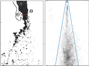
Figure 3. DI back-lit images in the near field. Black lines indicate gas streamlines. Relatively low (high) pressure regions indicated by encircled  $p_-$ (
 $p_+$), red arrow indicates restorative force initiating flapping; (a)
  $M=25.3$ (b)
  $M=81.2$. DI forward-scattering images in the near and far fields for (c)
  $M=25.3$ and (d)
  $M=81.2$. The solid blue lines indicate the ten per cent width (
 $r_{0.1}/d_g$).
These radial excursions are quantified by investigating the likelihood of liquid occupying a given position in the flow field, calculating its probability of presence ( $P$) over the entire time of study. The method is detailed in Machicoane et al. (Reference Machicoane, Ricard, Osuna-Orozco, Huck and Aliseda2020) in the same facility presented here. Background-corrected images appear nearly binary due to the strong density interface between the gas, which appears as a
  $0$, and the liquid as a
  $1$. A threshold background-corrected pixel value of 0.5 is chosen to create a binary image, although this value does not significantly impact the results. The arithmetic average of each pixel gives
  $P$ for a statistically significant number of independent realizations. The complementary background-corrected images are presented in figure 3 for ease of viewing. In figure 4(a) the logarithm of
  $P$ is plotted and values corresponding to
  $P=1$ appear in black and indicate locations only occupied by liquid. Values corresponding to
  $P=0$ appear in white where liquid is never present. Radial slices through this plane are plotted, normalized by the probability at the centreline (
 $P_0$), in figure 4(b). Representative slices (in black) throughout the near field were found to be well approximated by a Gaussian profile centred on
  $r=0$ (in red) and are therefore fully characterized by the standard deviation
  $\sigma$.

Figure 4. Quantification of spreading in the near field. (a) Average map giving the logarithm of the probability of liquid presence for  $M=25.3$. Black corresponds to
  $P=1$ and white to
  $P=0$. (b) Black lines are slices (in linear scaling) through the average map at
  $x/d_g=[0.5, 1.0,1.5,2.0]$ for
  $M=25.3$. Plots have been shifted for clarity. Red lines are Gaussian fits where the symbols (
 $\bullet$,
  $\blacksquare$,
  $\blacklozenge$,
  $\blacktriangle$) correspond to
  $2\sigma$ at each position (
 $x/d_g=[0.5,1.0,1.5,2.0]$). (c) Evolution of
  $2\sigma$ profiles with downstream distance for a representative sample of momentum ratios. (d) Opening angle of the spray normalized by the opening angle of the gas phase. The dashed lines correspond to the correlation
  $\theta _{2\sigma }=59.9-10.6\times \log (M)$.
The radial extent of the spray is approximated by the local value of  $2\sigma$ which bounds 95.45 % of the liquid presence when symmetry about the centreline is accounted for. Figure 4(c) represents the evolution of the
  $2\sigma$ profile in the near-field region for a few representative momentum ratios. The sudden increase in width of the profiles for
  $x/d_g>0.25$ continues until the location where liquid detaches from the intact liquid core. This position, called the intact length, is marked by the symbols in figure 4(a) using the correlation in Machicoane et al. (Reference Machicoane, Ricard, Osuna-Orozco, Huck and Aliseda2020). However, optical occlusion of the intact core prevents the exact determination of the intact lengths for
  $M=[177,376]$ and they are estimated by the minima in the
  $2\sigma$ profiles. A critical value of
  $M\approx 50$ was identified by Lasheras & Hopfinger (Reference Lasheras and Hopfinger2000) where the intact length is truncated by a recirculating gas cavity that creates a hollow core in the intact liquid jet (see figure 9c in Machicoane et al. (Reference Machicoane, Bothell, Li, Morgan, Heindel, Kastengren and Aliseda2019)) and limits the progression of the intact length towards the nozzle. The gas streamlines of this process are sketched in figure 3(b). At the highest momentum ratios (
 $M>81.2$), the liquid core essentially acts as a backward-facing step when streamlines separate from the truncated liquid core (sketched in figure 3b). Spectral content is likely broadband, with frequencies originating from the vortices shedding from the shear layer, as well as lower frequencies from the instability of the cavity itself similar to a backward-facing step (Eaton & Johnston Reference Eaton and Johnston1980, Reference Eaton and Johnston1982). Flapping and oscillation due to an unsteady recirculating gas cavity are separate phenomena affecting the liquid core, and are characteristic of low and high momentum ratios (respectively) with the transition occurring at
  $M\approx 50$.
Calculating a linear regression for  $x/d_g=[1.5 - 2.25]$ in figure 4(c), we quantify the spreading rate (
 $S_{2\sigma }$) and then calculate the opening angle of the spray
 \begin{equation} {\theta_{2\sigma}=2\tan^{{-}1}(S_{2\sigma}),} \end{equation}
plotted in figure 4(d) against the spreading angle of the gas phase  $\theta _{0.1}^U$. Interestingly, for
  $M\lesssim 40$, the dispersed liquid in the near field has a greater spreading angle than the gas phase, while for
  $M\gtrsim 40$, the spray has a lower spreading angle than the gas phase. We note that the critical momentum ratio
  $M\approx 40$ is indicative of the overall trend and is close to the critical value of
  $M=50$ given by Lasheras & Hopfinger (Reference Lasheras and Hopfinger2000).
Caution should be taken when interpreting the highest momentum ratios ( $M>176.6$). We expect that the lateral extent of the average profiles to be slightly underestimated due to the coarse image resolution (
 $29\,\mathrm {\mu }\textrm {m}\,\textrm {pixel}^{-1}$) with respect to the smallest droplets (arithmetic average
  $d_{10}<10\, \mathrm {\mu }$m) and to image blur related to the exposure time of the camera (0.3
  $\mathrm {\mu }$s). The opening angle
  $\theta _{2\sigma }$ would be expected to deviate more strongly from the dashed line if all droplets were resolved and we interpret these angles as lower bounds that account for larger, mass-carrying droplets.
The amplification or suppression of strong radial excursions by the intact liquid core is expected to play a strong role in determining the mixing of the droplet phase in the far field of the jet. It can be seen that large droplets are ejected from the jet's core at the nozzle (figure 3a) and are found beyond the ten per cent width (blue lines) in figure 3(c) for  $M=25.3$. At higher momentum ratios (
 $M=81.2$), droplets are more confined toward the centreline (figure 3d). In the next section, we investigate the dispersion of liquid mass throughout the jet via PDI measurements.
5. Spray structure in the far field
The interactions of the gas and liquid phases at the intact liquid–jet interface explain the narrowing of the spray in the near field. Subsequent droplet advection into the far field ( $7< x/d_g<45$) is described by the evolution of the volume fraction (VF:
  $\phi$) and volume-flux density (VFD:
  $\dot {g}$) and are discussed in this section.
5.1. VFD and VF definitions
The VFD is calculated for each diameter class, i, containing a total number  $N_{i}$ of droplets
 \begin{equation} \dot{\mathcal{G}}(d_i)=\frac{\rm \pi}{6T_s{\mathcal{A}_{i}}}\sum_{j=1}^{N_{i}}{d_{j,i}^3} , \end{equation}
where  $T_s$ is the total sample time,
  $\mathcal {A}_{i}$ is the probe cross-section (2.1) of the
  $j$th droplet of the
  $i$th size class with diameter
  $d_{j,i}$. We can calculate the VF assuming a single droplet occupies the probe volume at a time for the
  $i$ droplet class
 \begin{equation} \varPhi(d_i)=\frac{\rm \pi}{6}\frac{\tilde{t}_i}{T_s{\mathcal{V}_i}}\sum_{j=1}^{N_{i}}{d_{j,i}^3}, \end{equation}
where  $\tilde {t}_i$ is the residence time of a droplet in the size-class probe volume
  $\mathcal {V}_i$ (2.2). Both (5.1) and (5.2) are defined over a given binned droplet size class. Between 15 and 21 binned size classes (index
  $i$) are used, with fewer bins used for higher momentum ratios
  $M$. A more general quantity obtained by integrating over all
  $D$ droplet size classes,
 \begin{equation} \dot{g}=\sum_{i=1}^D\dot{\mathcal{G}}(d_i), \end{equation}
is the VFD for all droplet size classes and,
 \begin{equation} \phi=\sum_{i=1}^D\varPhi(d_i), \end{equation}
the VF for all droplet size classes. These quantities are understood to be time averages of instantaneous values of VFD and VF.
It is important to note that not every drop passing through the PDI probe volume is captured. Due to the Gaussian nature of the laser beam, smaller droplets scatter less light than large droplets at the beam's edge. We correct for the bias that arises in the flux and VF measurements by introducing size-dependent probe areas (2.1) and volumes (2.2). Other biases such as multiple droplets and non-spherical droplets in the probe volume as well as multi-mode scattering are corrected for (Bachalo Reference Bachalo1994) but lead to a sub-sampling of the droplet population. When the VFD (5.4) is integrated over the spray cross-section for different downstream locations and the total volume flux is measured, values are found around [12.5–25] % of the nominal value at the nozzle for each momentum ratio. Similarly, the droplet-size distributions averaged over the spray cross-section to give an arithmetic mean diameter,  $d_{10}$, vary by at most 8 % of the average value over all downstream locations. Consistency in the area-averaged volume flux and diameter measurements in the far field indicate that, despite the fact that the PDI subsamples the droplet population in the spray, these measurements are unlikely to introduce a bias in the droplet populations.
5.2. VFD and VF profiles
The VF and VFD, normalized by their maximum values for different momentum ratios, are plotted against the self-similar coordinate  $\eta =r/(x-x_0^{\scriptscriptstyle \langle U\rangle })$ in figure 5 for different distances downstream of the nozzle. Increasing the gas flow rate (increasing
  $M$) narrows both the VFD (figure 5a) and the VF (figure 5b) profiles, as observed with similar co-axial atomizers (Hardalupas & Whitelaw Reference Hardalupas and Whitelaw1993, Reference Hardalupas and Whitelaw1994; Engelbert et al. Reference Engelbert, Hardalupas and Whitelaw1995). An important difference between the VFD and VF is that the former is narrower than the latter over the range of momentum ratios investigated, in line with earlier observations (Hardalupas, Taylor & Whitelaw Reference Hardalupas, Taylor and Whitelaw1989) in a particle-laden jet. While the VFD is always narrower than the average velocity profile (figure 5a), the VF profile straddles the velocity profile (figure 5b) depending on the momentum ratio. For a critical momentum ratio,
  $M\approx 56$, the average concentration profile roughly follows the average velocity profile.

Figure 5. Comparison of VFD,  $\dot {g}$, and VF,
  $\phi$. (a,b) VFD and VF normalized by value at centreline plotted against the self-similar coordinate
  $\eta =r/(x-x_0)$ for
  $x/d_g=[9, 12, 18, 24]$. The momentum in the liquid phase is constant while varying gas-phase momentum
  $M=[25, 56, 177]$.(c,d) VF and VFD profiles are normalized by the ten per cent width coordinate defined in (5.5) at
  $x/d_g=[18]$.
For each momentum ratio plotted in figure 5, profiles from different downstream locations collapse onto a single curve, when the self-similar coordinate  $\eta$ is used. We denote this self-similar region the ‘far field’, occurring roughly from
  $7< x/d_g<45$, in agreement with the PLJ observations in Picano et al. (Reference Picano, Sardina, Gualtieri and Casciola2010). Although this parameter accounts for the self-similarity of the profiles with downstream distance, it does not account for variation in profile shape as the momentum ratio is varied. Using the 10 per cent width defined as
 $$\begin{gather} \dot{g}(r_{0.1}^{\dot{g}})=0.1\dot{g}_{max}, \end{gather}$$
 $$\begin{gather}\phi(r_{0.1}^\phi)=0.1\phi_{max}, \end{gather}$$
 $$\begin{gather}\langle U\rangle(r_{0.1}^U)=0.1\langle U\rangle_{max}, \end{gather}$$
we normalize the VF and VFD in figure 5(c,d). We focus on the 10 per cent width because it was found to be more sensitive to momentum-ratio-dependent changes in the tails of the curves (e.g. figure 5a,b) than the more common half-width metric. The normalized VF and VFD profiles display a satisfactory collapse at  $x/d_g=18$ in figure 5(c,d). This collapse indicates that the momentum-ratio-dependent physics governing the shape of the VF and VFD profile is captured by an appropriate choice of a self-similar variable in agreement with observations in the literature (Picano et al. Reference Picano, Sardina, Gualtieri and Casciola2010; Lau & Nathan Reference Lau and Nathan2016).
For all  $M$, the 10 per cent widths (both VF and VFD, figure 5a,b) evolve linearly in the far field of the jet. In general, as the momentum ratio increases, the width of the spray (either by VFD or VF) is narrower, similar to Engelbert et al. (Reference Engelbert, Hardalupas and Whitelaw1995). Near the critical momentum ratio,
  $M\approx 56$, we find that
  $r_{0.1}^\phi \approx r_{0.1}^U$. For
  $M>56$, we find that
  $r_{0.1}^\phi < r_{0.1}^U$ and for
  $M<56$ that
  $r_{0.1}^\phi > r_{0.1}^U$, in accordance with the self-similar VFD profiles in figure 5(a–d),
  $r_{0.1}^\phi >r_{0.1}^{\dot {g}}$ for all
  $x/d_g$.
Both the VFD and VF are governed by the spreading rate in the far field of the turbulent jet and are defined in a similar manner to the spreading rate of the velocity profile in (3.3)
 $$\begin{gather} S_{0.1}^{\dot{g}}={\textrm{d} r_{0.1}^{\dot{g}}}/{\textrm{d}\kern0.06em x}, \end{gather}$$
 $$\begin{gather}S_{0.1}^{\phi}={\textrm{d} r_{0.1}^\phi}/{\textrm{d}\kern0.06em x}, \end{gather}$$
 $$\begin{gather}S_{0.1}^{U}={\textrm{d} r_{0.1}^U}/{\textrm{d}\kern0.06em x}. \end{gather}$$
We take the spreading rate to be the value of  $\eta$ where the seventh-order polynomial interpolation of
  $\phi /\phi _{max}$ and
  $\dot {g}/\dot {g}_{max}$ in figure 5(a,b) reaches 10 %. Similar values are obtained from a linear fit of figure 6(a). The opening angle of the VFD, VF and velocity with respect to the 10 per cent width is given by
 $$\begin{gather} \theta_{0.1}^{\dot{g}}=2\tan^{{-}1}(S_{0.1}^{\dot{g}}), \end{gather}$$
 $$\begin{gather}\theta_{0.1}^{\phi}=2\tan^{{-}1}(S_{0.1}^{\phi}), \end{gather}$$
 $$\begin{gather}\theta_{0.1}^{U}=2\tan^{{-}1}(S_{0.1}^{U}).\end{gather}$$
The evolution of the opening angles of each metric with respect to the opening angle of the jet  $\theta _{0.1}^U=20.6^\circ$ is plotted in figure 6(b) as a function of momentum ratio. Data for constant liquid flow rate and variable gas flow rate (blue) and constant gas flow rate and variable liquid flow rate (shades of grey) are given. For all momentum ratios, we observe that the opening angle of the VFD profiles is smaller than the VF. The opening angle decreases with increasing momentum ratio and, past
  $M\approx 10$, follows a logarithmic trend. The critical momentum ratio
  $M\approx 56$ is observed to indicate the threshold beyond which the VF profiles spread less than the gas phase. Due to the agreement of the observations of critical behaviours in spreading rates of liquid presence and VF in both near and far field, respectively, we define an overall critical momentum ratio of
  $M_c=50$.

Figure 6. Evolution of VFD and VF profiles. (a) Normalized 10 per cent width compared against the self-similar jet solution (dashed line) for  $M=[25, 56, 177]$. (b) Opening angles calculated of the VF/VFD profiles normalized by the opening angle (5.11) of the gas phase. Points in blue correspond to
  $Re_L=1050$, in light grey to
  $Re_L=2900$ and
  $M=5.1$,and dark grey to
  $Re_L=4770$ and
  $M=1.9$. Solid (dashed) line describes the logarithmic trend as
  $\theta _{0.1}^{\phi }/\theta _{0.1}^U=1.625-0.153\log (M)$ (
 $\theta _{0.1}^{\dot {g}}/\theta _{0.1}^U=1.625-0.153\log (M)$); (inset) difference in opening angle of VF and VFD with respect to the opening angle of the gas.
The logarithmic dependency of  $\theta _{0.1}^{\dot {g}}$ and
  $\theta _{0.1}^\theta$ will not continue to arbitrarily large
  $M$ because the opening angles cannot be negative. The opening angles of the VF profiles tend toward that of the VFD (figure 6b, inset) suggesting that an asymptotic regime where
  $\theta _{0.1}^{\dot {g}}/\theta _{0.1}^{\phi }\rightarrow 1$ and
  $\theta _{0.1}^{\dot {g}}/\theta _{0.1}^{U}<1$ is likely. This is because radial transport of the droplet phase is sustained by the radial transport of gas momentum. Thus, for arbitrary
  $M$, the radial expansion of the VFD profile may approach, but not exceed, the radial expansion of the gas-phase profile.
6. Droplet presence at the spray's edge
In this section, the presence of large droplets on the spray's edge is linked to their inertia with respect to the large-scale structures in the spray. This framework permits of description of the radial droplet-size profiles within the broader context of the parameter range of turbulent round-jet sprays (§ 7).
6.1. Liquid ligament ejection
In figure 3(c,d), two sprays are imaged, one where  $M< M_c$ and the other with
  $M>M_c$. In the far field of the former, at
  $x/d_g\approx 24$, droplets are clearly detected beyond the edge of the gas jet (
 $r_{0.1}^U/d_g=4.8$) given by the blue lines, with some even observed near
  $r/d_g=\pm 10$. For
  $M< M_c$, large droplets can be found on the jet's edge, however, the finite resolution of the images and weak light scattering by small particles may obscure their presence in these images.
To confirm the dominance of large drops near the edge of the spray for  $M< M_c$, probability density functions (p.d.f.s) were calculated for
  $M=25$ at four downstream locations for
  $r\sim 1.5r_{0.1}$ in figure 7(a). With the exception of
  $x/d_g=36$, each p.d.f. displays a peak for diameters much larger (
 $d>66\,\mathrm {\mu }\mathrm {m}$) than the typical peak of the spray droplet-size distribution near the centreline (
 $d= {\textit{O}}(10\,\mathrm {\mu }\mathrm {m})$, figure 7a, inset). We refer to the droplets constituting the secondary peaks at the spray's edge as ejections. This peak diameter increases in size with downstream distance until
  $x/d_g=36$, where it shifts back to a smaller droplet diameter. Beyond
  $M\approx M_c$, no peak corresponding to an ejection is observed.

Figure 7. Characterization of droplet-size p.d.f.s on the spray's edge: (a) p.d.f.s for  $M=25.3$, radial position
  $r\sim 1.5r_{0.1}$, downstream position
  $x/d_g=[9,18,24,36]$, ([
 $\bullet$,
  $\blacksquare$,
  $\blacktriangle$,
  $\blacklozenge$] respectively). The p.d.f.s display a predominant mode that is characteristic of
  $M=[25.3, 39.2, 56.0]$ except for
  $x/d_g=36$; (inset) p.d.f.s at
  $r/d_g=0$ with modes of
  $ {\textit{O}}(10\,\mathrm {\mu }\mathrm {m})$. Symbols correspond to downstream position. (b) The droplet size corresponding to the mode when
  $r\sim 1.5r_{0.1}$,
  $d_{p,peak}$, is assigned the characteristic droplet time scale
  $\tau _{p,peak}=\rho _\ell d_{p,peak}^2/(18\nu _g\rho _g)$ and compared with the integral scale
  $T_E$ (6.1).
This phenomenon can be explained by the interaction of ejections with the largest eddies of the turbulent jet. The role of the eddies in selectively transporting droplets was proposed by Chung & Troutt (Reference Chung and Troutt1988) and subsequently experimental (Lazaro & Lasheras Reference Lazaro and Lasheras1992a; Longmire & Eaton Reference Longmire and Eaton1992) and numerical (Sbrizzai et al. Reference Sbrizzai, Verzicco, Pidria and Soldati2004) investigations in different shear-driven flows have largely supported this hypothesis. These eddies are characterized by an Eulerian time scale
 \begin{equation} {T_E={2r_{0.1}}/{u^\prime},} \end{equation}
where  $u^\prime$ is the longitudinal velocity fluctuations on the centreline and
  $2r_{0.1}$ approximates the diameter of the gas jet at a given downstream position. This length scale is chosen because the literature suggests the presence of large axisymmetric and helical structures (Dimotakis, Miake-Lye & Papantoniou Reference Dimotakis, Miake-Lye and Papantoniou1983; Mungal & Hollingsworth Reference Mungal and Hollingsworth1989) that persist into the far field of the jet and are correlated over its width (Tso & Hussain Reference Tso and Hussain1989; Yoda, Hesselink & Mungal Reference Yoda, Hesselink and Mungal1992). Similar definitions of
  $T_E$ have been used (Prevost et al. Reference Prevost, Boree, Nuglisch and Charnay1996) to characterize large-scale motions over the entire jet cross-section.
The ejections for  $M=[25,~39,~56]$ are used to calculate a time scale based on the characteristic diameter at the peak
  $d_{p,peak}$ in figure 7(a)
 \begin{equation} {\tau_{p,peak}=\rho_\ell d_{p,peak}^2/(18\nu_g\rho_g)}, \end{equation}
and are plotted as a function of their local Eulerian time scale  $T_E$ in figure 7(b). The ejections collapse on a single line whose slope gives a Stokes number characteristic of the ejections
 \begin{equation} St_{peak}={\tau_{p,peak}}/{T_E}. \end{equation}
A slope of  $St_{peak}=1.9$ is measured and is of order one, strongly suggesting that large eddies are responsible for the presence of liquid ejections on the edge of the spray.
Experimental evidence in PLJs (Hardalupas et al. Reference Hardalupas, Taylor and Whitelaw1989) and sprays (Engelbert et al. Reference Engelbert, Hardalupas and Whitelaw1995) suggests that the initial conditions seen by a particle at injection determine a ballistic trajectory until the local Stokes number with respect to the large energy containing scales becomes of order one. In the case when  $M< M_c$, the radial velocity associated with the flapping instability sends droplets on ballistic trajectories as they are ejected from the jet. Then, droplets travelling downstream for which
  $St< St_{peak}$ would be less probable at the spray edge because they have been re-entrained on the upstream side of the eddy where the entrainment process is strongest (Lampa & Fritsching Reference Lampa and Fritsching2013). Such an entrainment process would culminate in predominantly smaller droplets on the spray's edge, explaining the shift to smaller droplet modes in the range
  $x/d_g=[24 - 36]$ in figure 7(a).
6.2. Ejection relaxation to the gas phase
To determine if droplets capable of interaction with large eddies exist within the spray, we have calculated the normalized and radially integrated VFD conditioned on droplet size. As opposed to the size-conditioned VFD at a given radial location (5.1), an integral VFD was calculated over successive annuli of the spray centred on the position of the PDI probe volume and weighted by the relative area of each annulus. The probability of finding droplets within the annulus is assumed to be statistically homogeneous. Finally, the conditioned and weighted VFD was normalized by the sum over all sizes. We call this normalized metric the VFD function (v.f.d.f.) and it is implied in the following section that it is a quantity integrated over a cross-section of the spray although it can also be evaluated locally (§ 7). The v.f.d.f. relates the VFD (volume per unit area and unit time) carried by a droplet with diameter between  $d$ and
  $d+\mathrm {d}(d)$. In fact, the v.f.d.f. contains the same information as the number flux density (number per unit area and unit time), commonly referred to as the p.d.f., and the two are analytically related (Appendix A).
Once atomization has occurred, and assuming coalescence and evaporation are negligible in the short residence times in the near- to far-field droplet trajectories, the v.f.d.f. remains essentially unchanged as the spray evolves downstream. Preserved values of arithmetic and volume-averaged diameters were taken to be an indication of high-quality PDI measurements in § 5.1 for this reason. The v.f.d.f.s are presented in figure 8(a) for  $M=[25.3 - 176.6]$ at
  $x/d_g=24$ but other locations collapse onto the same curve. Narrowing of the v.f.d.f. with increasing
  $M$ is characterized by a decrease in the
  $d_{43}^i$ (mass-flux-weighted) diameter which is the first moment of the v.f.d.f. (B3). The superscript
  $i$ indicates that the v.f.d.f. is integrated over the spray cross-section and its first moment (
 $d_{43}^i$) is a global characteristic of the spray at a given downstream location
  $x/d_g$. Absence of the superscript indicates that the v.f.d.f. is evaluated at a given downstream and radial location and its first moment (
 $d_{43}$) is a local characteristic of the spray. The
  $d_{43}^i$ follow a power law
  $d_{43}^i\propto M^{-0.79}$ and are plotted in figure 8(b).

Figure 8. Radially integrated measurements taken at  $x/d_g=24$ characteristic of the entire spray cross-section. (a) The v.f.d.f. for different momentum ratios. Solid lines correspond to (6.5) with
  $n=3.9$. (b) First moment of the v.f.d.f. evaluated over the spray cross-section,
  $d_{43}^i$, at
  $x/d_g=24$ for various
  $M$.
$M$.
Interestingly, the v.f.d.f. can be described by a single parameter gamma function
 \begin{equation} \varGamma(n,x=d/d_{43}^i)=\frac{n^n}{\varGamma(n)}x^{n-1}\exp({-}nx), \end{equation}
which gives the following approximation:
 \begin{equation} \mathrm{v.f.d.f.}(d)=\frac{1}{d_{43}^i}\varGamma(n,d/d_{43}^i), \end{equation}
as observed by solid lines in figure 8(a). The v.f.d.f.s can be collapsed onto a single master curve given by (6.5) using  $n=3.9$ and
  $d_{43}^i$ in figure 8(b). This implies that, for both
  $M< M_c$ and
  $M>M_c$, sprays are governed by the same atomization mechanism, which has been attributed to the dynamics of ligaments formed by the co-axial gas jet (Marmottant & Villermaux Reference Marmottant and Villermaux2004; Villermaux, Marmottant & Duplat Reference Villermaux, Marmottant and Duplat2004).
The mass-flux-weighted average diameter  $d_{43}^i$ is indicative of the characteristic droplet carrying the overall mass flux in the spray. The characteristic time scale based on this droplet size class is
 \begin{equation} \tau_{43}={\rho_\ell}({d_{43}^{i}})^2/({{\rho_g}18\nu_g}). \end{equation}
A comparison of  $T_E$ and
  $\tau _{43}$ at
  $x/d_g=18$ for several momentum ratios is plotted in figure 9(a). If a droplet is resonant with the large eddies, then
  $\tau _{43}\sim T_E$. If
  $\tau _{43}> T_E$, there must be some droplets for which
  $\tau _{43}\sim T_E$ and ejections at the spray's edge are likely. However, if
  $\tau _{43}< T_E$, it is assumed that there are no droplets in the spray resonant with the large eddies and no, or few, ejections exist.

Figure 9. Evolution of area-averaged droplet time scale with  $M$ and
  $x/d_g$. (a) The droplet response time
  $\tau _{43}$ based on the
  $d_{43}^i$ diameter and the large-eddy time scales
  $T_{E}$ vary as a function of
  $M$. Dashed line is
  $\tau _{43}\approx 5.3\times 10^3 M^{-1.58}$ and the solid line is
  $T_E\approx 70.4\times M^{-0.50}$. (b) Evolution of the Stokes number for the peak probability droplet, as a function of the momentum ratio. Different symbols represent different downstream locations. Values above
  $St_{43}=1.9$ represent combinations where ejections are possible, values below
  $St_{43}=1.0$ are combinations where ejections are unlikely.
Evolution in droplet interactions with the large-scale eddies at a given  $x/d_g$ is captured by a global Stokes number
 \begin{equation} St_{43}=\tau_{{43}}/T_E. \end{equation}
For a given momentum ratio  $M$ in figure 9(b),
  $St_{43}$ decreases with downstream location because
  $\tau _{43}$ is constant and
  $T_E\propto (x/d_g)^2$. The range
  $St_{43}>St_{peak}$ (
 $St_{peak}=1.9$) corresponds to strongly inertial droplets and high ejection probability on the spray edge. The area bounded by dashed lines,
  $1< St_{43}< St_{peak}$, corresponds to a transitional regime where ejections become less probable on the spray edges. Below the solid line,
  $St_{43}<1$, droplets are weakly inertial with respect to the large eddies and ejection presence on the spray edges is unlikely. These observations are consistent with the momentum ratio and location where ejections were observed in figure 7.
7. Spray regimes
While the v.f.d.f. can be evaluated over the entire spray cross-section (§ 6.2), it can also be evaluated locally for a given downstream location ( $x/d_g$) and radial location normalized by the jet velocity ten per cent width (
 $r/r_{0.1}$). Profiles of first moment of the locally evaluated v.f.d.f., or the mass-flux-weighted (
 $d_{43}$) diameter, are investigated and used to characterize spray regimes that broadly fall into momentum ratio ranges:
  $M< M_c$,
  $M\approx M_c$ and
  $M>M_c$. To highlight their relationship with the large-scale flow features,
  $d_{43}$ profiles are normalized by a fictive droplet that would be resonant with the local large-scale eddy,
 \begin{equation} {\tilde{d}=(T_E18\nu_g\rho_g/\rho_\ell)^{1/2}.} \end{equation}
This normalization masks an important aspect of the  $d_{43}$ profile evolution with downstream location. For all
  $M$, the value of
  $d_{43}$ slightly increases on the centreline as the spray evolves downstream. This is a consequence of the large droplets on the centreline dispersing slower than smaller ones and therefore making a stronger statistical contribution on the centreline as the spray evolves. We note that, by definition,
  $(d_{43}/\tilde {d})^2$ is the local equivalent to the global Stokes number (
 $St_{43}$) defined in (6.7).
7.1. The case  $M< M_c$

For the momentum ratios below  $M_c$, the
  $d_{43}$ profiles retain a ‘
 $\cup$’ shape where the smallest droplets are found near the centreline and the largest near the edge (figure 10a–c). Within this range of
  $M$, slight differences are observed between
  $5.1< M< M_c$ (figure 10b,c) and
  $M<5.1$ (figure 10a).

Figure 10. Evolution of  $d_{43}/\tilde {d}$ profiles where
  $\tilde {d}=(T_E18\nu _g\rho _g/\rho _\ell )^{1/2}$ corresponds to a droplet with a characteristic time scale equal to the local Eulerian time scale
  $T_E$. Radial position is normalized by the
  $10\,\%$ width of the gas jet as an estimate of its radius. Solid lines correspond to
  $(St)^{1/2}=(1.9)^{1/2}=1.4$, the Stokes number corresponding to ejections; (a)
  $M=1.9$, (b)
  $M=5.1$, (c)
  $M=25.3$, (d)
  $M=56$, (e)
  $M=81.2$, (f)
  $M=176.6$, (f,inset)
  $M=176.6$, reduced ordinate range emphasizing central maximum.
When  $M<5.1$ there is a non-monotonic increase in
  $d_{43}$ from the centreline to the edge. There appears to be a local peak in
  $d_{43}$ near the centreline which falls off until
  $r\sim r_{0.1}$ and the droplet diameter increases again beyond the edge of the jet, where a maximum occurs. Similar profiles were observed by Engelbert et al. (Reference Engelbert, Hardalupas and Whitelaw1995) and were attributed to a delayed atomization characteristic of low momentum ratios. When break-up of the liquid core eventually occurs, it takes place further downstream in an environment with weaker shear. Large detached liquid ligaments form, which are subsequently atomized inefficiently, leading to large droplets on the centreline. Smaller droplets towards the edge are a result of their faster response to the jet turbulence. However, droplets even larger than those on centreline are found near the edge. These are likely the result of a flapping mechanism similar to the one established for larger
  $M$ sprays.
For  $5.1< M< M_c$, there is a monotonic increase in
  $d_{43}$ towards the edge of the spray (figure 10c). As suggested by Hardalupas et al. (Reference Hardalupas, Taylor and Whitelaw1989) and Engelbert et al. (Reference Engelbert, Hardalupas and Whitelaw1995), initial injection conditions lead to ballistic trajectories which persist until the droplets reach resonance with large eddies, typically for
  $d_{43}/\tilde {d}<(St_{peak})^{1/2}$. From figure 10(b,c) flattening in the profiles occurs when the droplets on the edge of the spray resides in the range
  $1< d_{43}/\tilde {d}<1.4$ similar to the range of droplet ejections that were hypothesized to interact with large-scale eddies in figure 9(b).
7.2. The case $M\approx M_c$

Close to  $M=M_c$, a confluence of factors affects the shape of the droplet diameter profiles. The liquid presence probability profiles (figure 4d) approach values determined by the gas-phase velocity profile, (
 $\theta _{2\sigma }\approx \theta _{0.1}^U$) which is thought to be due to suppressed flapping as
  $M$ approaches
  $M_c$. As a consequence, there are fewer large droplets on the spray edge and the VF profile in the far field (figure 6b) tends toward the gas-phase velocity profile (
 $\theta _{0.1}^\phi \approx \theta _{0.1}^U$). In figure 10(d), the diameter profile for
  $M=56$ is plotted and only at
  $x/d_g=12$ do the diameter profiles both present the signature of ejections with a prominent central minimum. For
  $x/d_g>12$, the integrated Stokes number is subcritical (
 $St_{43}< St_{peak}$), and nearly all of the radial values fall below the ejection threshold
  $d_{43}/\tilde {d}=(1.9)^{1/2}$. As the droplets continue downstream the profiles begin to flatten which is indicative of droplets relaxing to the gas phase (
 $St_{43}<1$).
7.3. The case $M\gg M_c$

The highest momentum ratio regime is characterized by a  $d_{43}$ profile with a central maximum and minima on the edges (figure 10f). As opposed to the
  $M< M_c$ regime, the flapping phenomenon does not significantly contribute to the dynamics of atomization nor does it impart initial radial momentum onto the droplets. In this regime, enhanced radial transport would be possible if droplets were resonant with the large eddies. However, the time scale of the droplets produced by atomization decreases with increasing
  $M$ (
$M$ ( $\tau _{43}\propto M^{-1.58}$) at a faster rate than eddy time scales decrease (
 $T_{E}\propto M^{-0.5}$) with increasing
  $M$ (increasing
  $Re_g$). This results in Stokes numbers for the droplet cloud well below unity. Due to the recirculating gas cavity present at
  $M\gg M_c$, larger droplets are confined to the centreline. The smallest droplets can follow the radial expansion of the gas phase closely. Thus, they are found more frequently near the edge of the jet, explaining the marked central maximum of
  $d_{43}$ and the minima on the edges.
7.4. Spray regime diagram ($We - Re_\ell$)

The data have been presented as a function of  $M=\rho _gu_g^2/(\rho _\ell u_\ell ^2)$ either by experimentally varying
  $u_g$ or
  $u_\ell$, independently. However, in § 7.3 it was seen that a convex (‘
 $\cap$’) profile with a central maximum could be observed both for low (
 $M=1.9$, figure 10a) and high momentum ratios (
 $M=[81.2, 176.6]$, figure 10e,f). Instead, the
  $We - Re_\ell$ phase space is introduced to account for gas- and liquid-phase momentum separately in the wider context of experimentally observed sprays.
PDI data from the literature presenting radial profiles of droplet size were surveyed (table 4). Results for the Sauter mean diameter ( $d_{32}$) we found, but not for the mass-flux-weighted diameter (
 $d_{43}$). From the present data, the evolution of
  $d_{43}$ is found to have less extreme differences between minima and maxima but, in general, the evolution described in §§ 7.1–7.3 for
  $d_{43}$ is similar for
  $d_{32}$. Since the profiles evolve downstream, the data displayed in the phase space are restricted to
  $x/d_g<13$.
Table 4. Experimental parameters from the literature, used in figure 11. Momentum ratio:  $M=\rho _g U_g^2/(\rho _\ell U_\ell ^2)$. Weber number:
  $We = \rho _g(U_g-U_\ell )^2d_\ell /\sigma$. Mass ratio:
  $m=\rho _\ell A_\ell U_\ell /(\rho _g A_g U)$. Liquid-phase Reynolds number:
  $Re_\ell =U_\ell d_\ell /\nu _\ell$. Gas-phase Reynolds number:
  $Re_g=U_g d_g/\nu _g$. Distance from nozzle where profile was measured:
  $x/d_g$. Diameter classes correspond to the Sauter mean diameter
  $d_{32}$ and mass-flux-averaged diameter
  $d_{43}$.

The phase-space diagram (figure 11) is divided into five regimes, colour coded based on the observed droplet diameter radial profile. Note that the solid symbols correspond to the PDI data in this paper. Regime I (red) corresponds to ‘∪’-shaped profiles. Regime II (yellow) corresponds to flat profiles. Regimes III (green), IV (blue) and V (grey) correspond to ‘ $\cap$’-shaped profiles. The white area is typically inaccessible to PDI measurements due to the inability of the spray to create spherical droplets in this regime.

Figure 11. Phase-space diagram ( $We - Re_\ell$) indicating the shape of the radial droplet profiles for the present experiments and those found in the literature, symbols are the same as in table 4, solid symbols are the present experiments. All of the points shown correspond to measurements within
  $x/d_{g}\leq 13$ and correspond to
  $d_{32}$ measurements except the present experiments (
 $d_{43}$). Colours are an indication of regime. Regime I (red) corresponds to ‘
 $\cup$’-shaped profiles. Regime II (yellow) corresponds to flat profiles. Regimes III (green), IV (blue) and V (grey) correspond to ‘
 $\cap$’-shaped profiles. The white area is typically inaccessible to PDI measurements due to the inability of the spray to create spherical droplets in this regime.
For  $Re_\ell \lesssim 4000$ and
  $50< We<300$, the profiles fall in regime I where flapping is dominant and gives rise to other morphologies such as ‘ladle’ (Eroglu & Chigier Reference Eroglu and Chigier1991) structures (figure 3a,c) which launch drops beyond the gas jet creating ‘
 $\cup$’-shaped profiles. Increasing the momentum in the gas phase for
  $Re_\ell \lesssim 4000$ and
  $We\gtrsim 300$ reduces the role of the flapping instability, marking the transition from regime I to II. This transition corresponds to
  $M=M_c$ for our data set and a flattening of the mass-flux-weighted diameter profile (figure 10d). If the momentum in the gas phase is increased beyond
  $We\sim 800$ (and
  $Re_\ell \lesssim 4000$), a transition between flat and ‘
 $\cap$’-shaped profiles occurs (II to III). This regime is characterized by the emergence of a recirculating gas cavity just downstream of the liquid core.
The present data ( $M<5.1$, figure 10a,b), help confirm the transition from regime II to IV that occurs for
  $200< We<800$ and
  $Re_\ell \approx 4000$. In regime IV there are large droplets near the spray edges and also on the centreline, giving ‘W’-shape profiles close to the transition at
  $Re_\ell \approx 4000$ (figure 10a). Further into regime IV, the gas phase lacks sufficient momentum to initiate the flapping instability and the instability transitions to the ‘dilational waves’ observed by Engelbert et al. (Reference Engelbert, Hardalupas and Whitelaw1995). These waves are sufficiently long lived for successive vortices to establish recirculation regions in the wake of the KH wave. In Zandian et al. (Reference Zandian, Sirignano and Hussain2018), vortex stretching leads to the formation of hairpin vortices in the wake region that deform these recirculating vortices which in turn deform the liquid core. This cascade gives rise to the droplets constituting ‘
 $\cap$’-shaped profiles.
Interestingly, these profiles in regime IV ( $Re_\ell \gtrsim 8000$) resemble profiles in regime III which are also ‘
 $\cap$’-shaped and also do not exhibit flapping due to the recirculating gas cavity. While at lower
  $We$ surface tension resists the formation of droplets, in the high
  $We$ regime the hairpin vortices described above are able to perforate the ligaments forming smaller droplets as described by Zandian et al. (Reference Zandian, Sirignano and Hussain2018). This mechanism helps us to understand the difference in droplet sizes between regime III and IV despite similarities in the profile shape.
Regime V is not explored in this paper and deserves comment. The boundary between regimes III and V is difficult to delimit as both display ‘ $\cap$’-shaped profile. Increasing the liquid momentum, and with it the liquid–gas mass ratio, in the spray when the gas momentum is high (
 $We>800$) results in increased transfer of momentum from gas to the liquid phase as more liquid is required to accelerate to the gas-phase velocity. This may change the nature of atomization that occurs after liquid separates from the intact core, known as secondary atomization (SA). Lasheras, Villermaux & Hopfinger (Reference Lasheras, Villermaux and Hopfinger1998) and Lasheras & Hopfinger (Reference Lasheras and Hopfinger2000) identify two mechanisms of SA-driven break up: mean shear and turbulence induced. The former occurs when a strong enough relative velocity occurs between the droplet and the gas while the latter is due to destabilizing turbulent fluctuations occurring over the droplet's surface. As more gas momentum is transferred to the accelerate the liquid phase, velocity fluctuations are dampened (Modarress, Wuerer & Elghobashi Reference Modarress, Wuerer and Elghobashi1984; Engelbert et al. Reference Engelbert, Hardalupas and Whitelaw1995) resulting in increasingly weak turbulent SA. This is thought to be the mechanism governing the spray transitions from regime III to V. However, the precise role of turbulent and shear SA in regimes III and V deserves further research.
8. Discussion and conclusions
The presence of ‘ $\cup$’, flat and ‘
 $\cap$’-shaped profiles is thought to be a consequence of the ability of the spray to progressively entrain ejections by large-scale eddies on the spray's edge. Figure 12 provides a conceptual sketch of the break-up and dispersion processes discussed in this paper.

Figure 12. Sketch of the break-up and dispersion processes. Flow separation at the interface causes recirculation in both (a)  $M< M_c$ and (c)
  $M>M_c$ cases. Large (L), medium (M) and small (S) droplets interact differently with a series of eddies (
 $E_0, E_1, E_2, E_3$) when
  $M< M_c$ and
  $M>M_c$; (a,b)
  $M< M_c$, (c,d)
  $M>M_c$.
Within the inner shear layer which forms between the liquid and gas jets at  $M< M_c$ (figure 12a), interfacial instabilities grow until the gas flow separates and recirculates behind the perturbation. Separation causes a pressure gradient to establish across the liquid jet (dark black) causing it to flap and produce liquid ligaments (medium grey) which form smaller stable droplets (light grey) that may be found far from the jet centreline. The dispersal of a ‘small’ (time scale:
  $\tau _{ps}$), ‘medium’ (
 $\tau _{pm}$) and ‘large’ (
 $\tau _{pl}$) droplet in the far field is depicted in figure 12(b).
The droplets travel with ballistic trajectories until they encounter eddies in the far field with the same sense of rotation as those originating in the outer shear layer formed between the co-axial gas flow and stagnant ambient fluid in the near field. Droplet trajectories are eventually perturbed by these far-field eddies  $E$ with time scales
  $[T_{E0},T_{E1},T_{E2},T_{E3}]$ based on (6.1). At
  $E_0$, all droplets are inertial such that
  $T_{E0}<\tau _{ps}<\tau _{pm}<\tau _{pl}$ and they overshoot the eddy. By virtue of its imminent entrainment,
  $\tau _{ps}$ is at the threshold for ejections at
  $E_0$ and
  $\tau _{ps}/T_{E0}\approx 1.9$ determined in § 6.1. At
  $E_1$, the smallest droplets are resonant with the eddies (
 $\tau _{ps}\approx T_{E1}$) and are entrained on the upstream side of the eddies. Meanwhile,
  $T_{E1}<\tau _{pm}<\tau _{pl}$ and the medium and large droplets continue ballistically with the new ejection threshold
  $\tau _{pm}/T_{E1}\approx 1.9$. The entrainment process continues at
  $E_2$, where the
  $\tau _{pm}\approx T_{E2}$ and
  $\tau _{pl}/T_{E2}\approx 1.9$. Finally, the large droplets are entrained at
  $E_3$ when
  $\tau _{pl}\approx T_{E3}$ leaving none of the initial ejections near the edge of the jet. The progressive entrainment of large droplets from the spray's edge is thought to be responsible for the flattening of the droplet-size profiles when
  $M< M_c$.
Due to the increased momentum in the gas phase, the inner shear layer establishes a recirculating gas cavity just downstream of the liquid jet (black shading) for  $M>M_c$ (figure 12c). The presence of this shear layer is responsible for liquid ligaments (medium grey) that are stripped from the intact liquid jet much earlier than for the
  $M< M_c$ case. These ligaments eventually break down into droplets (light grey), which are concentrated in the vicinity the gas jet's centreline (dotted line). The large droplets are essentially ballistic and deviate very little from the centreline while the smallest droplets are more sensitive to large eddies and can be transported radially (figure 12d). In this regime,
  $St_{43}\lesssim 1$ and as the droplets travel downstream they become less inertial and begin to follow the gas phase, causing them to be swept into the downstream side of the outer shear-layer eddies. This creates the ‘branching’ pattern at the sprays edge in figure 3(d) as the droplets are transported toward the spray's exterior. Similar observations have been made in droplet-laden two-dimensional shear layers (Lazaro & Lasheras Reference Lazaro and Lasheras1992a), as well as in co-axial atomizers (Lampa & Fritsching Reference Lampa and Fritsching2013). Despite the droplets interacting with large-scale structures at
  $M>M_c$, the spray is significantly narrower due in large part to the liquid core's inability to shed droplets far from the centreline, as is the case for
  $M< M_c$.
The ratio of mass-flux-weighted diameter ( $d_{43}^i$) to the diameter of the droplet that would be resonant with a local large eddy (
 $\tilde {d}$) allows an a priori estimation of the mass-flux-weighted droplet-size profiles that develop in the dispersion regimes above. Profiles with a predominant central minimum and edge minima (
 $d_{43}^i/\tilde {d}>1.4$,
  $M< M_c$) arise when ejections are found at the spray's edge due to flapping. For momentum ratios close to the critical value (
 $M\approx M_c$), mostly flat profiles arise for
  $0.6\lesssim d_{43}^i/\tilde {d}\lesssim 1.4$. For
  $M>M_c$, suppressed flapping and the absence of ejections result in profiles with a predominant central maximum and edge minima arise with
  $d_{43}^i/\tilde {d}\lesssim 0.6$.
This paper experimentally investigated the dispersion regimes in the far field of a spray produced by a co-axial two-fluid atomizer. It was found that the presence of known atomization mechanisms in the near-nozzle region strongly impacts the dispersion of droplets in the far field. A critical momentum ratio of  $M_c=50$ separates a regime with significant liquid presence beyond the edge of the gas jet (
 $M< M_c$) from a regime with most of the liquid confined within the gas jet boundaries (
 $M>M_c$). To the best of the authors’ knowledge, and despite the maturity of the spray physics field, no explanation for the rich variety in droplet-size profiles found in the literature has yet been given. We have linked the above regimes to three classes of droplet-size profile shapes and established a framework for predicting them based on relevant spray parameters. Amongst these, the critical Stokes number
  $St=\tau _p/T_E=1.9$ indicates droplets that are susceptible to dispersing beyond the nominal extent of the gas phase. The ability to predict evolving spray shape with different gas/liquid parameters may prove useful in various spray control applications where a dynamically varying spray with known characteristics may be required (Osuna-Orozco et al. Reference Osuna-Orozco, Machicoane, Huck and Aliseda2019, Reference Osuna-Orozco, Machicoane, Huck and Aliseda2020).
Funding
This work was sponsored by the Office of Naval Research (ONR), as part of the Multidisciplinary University Research Initiatives (MURI) Program, under grant number N00014-16-1-2617.
Declaration of interests
The authors report no conflict of interest.
Appendix A. Relationship between p.d.f. and v.f.d.f.
Intuition suggests that the p.d.f. and v.f.d.f. are related. The former expresses the probability that a certain number of droplets is observed, the latter that a volume is observed. Below, we show that that the p.d.f. is mathematically equivalent to the normalized number flux density function n.f.d.f. We prefer to use the number density function (n.f.d.f.) rather than the p.d.f. as it specifies how the measurements were made (i.e. per unit area per unit time). We show that the n.f.d.f. and v.f.d.f. are related analytically.
The probe cross-sectional area can be written  $\mathcal {A}_{i}=L\ell =L\bar {\ell }(1+b_i)$ where
  $b_i=(1+(\ell _i-\bar {\ell })/\bar {\ell })$ relative to the
  $i$th droplet diameter class with probe length
  $\ell _i$ given an average probe length
  $\bar {\ell }$. The VFD per size class is given by,
 \begin{equation} \dot{\mathcal{G}}(d_i)=\frac{\rm \pi}{6T_s\bar{\mathcal{A}}(1+b_i)}\sum_{j=1}^{N_{i}}d_{ij}^3 , \end{equation}
where  $\bar {\mathcal {A}}=L\bar {\ell }$. Note that the factor
  $(1+b_i)$ acts as a multiplicative constant related to the bias towards large droplets in particle counting systems. It corrects for an overestimation of large droplets as the path length
  $\ell$ for small droplets is smaller than for large droplets. The VFD summed over
  $D$ total size classes is
 \begin{equation} \dot{g}=\sum_{i=1}^D\dot{\mathcal{G}}(d_i). \end{equation}
The unbiased volume-averaged diameter is calculated as,
 \begin{equation} d_{30}=\left(\left(\sum_{i}^{D}(1+b_i)^{{-}1}\sum_{j}^{N_i} d_{ij}^3\right) \left(\sum_{i}^{D}(1+b_i)^{{-}1}\sum_{j}^{N_i} 1\right)^{{-}1}\right)^{1/3}. \end{equation}
Normalization of the VFD gives the VFD function (v.f.d.f.),
 \begin{equation} \mathrm{v.f.d.f.}(d_i)=\frac{\dot{\mathcal{G}}(d_i)/\mathrm{d}d}{\dot{g}}=\frac{1}{\mathrm{d}d}\sum_{j=1}^{N_{i}}\frac{d_{ij}^3}{(1+b_i)}\left(\sum_{i=1}^D\sum_{j=1}^{N_{i}}\frac{d_{ij}^3}{(1+b_i)}\right)^{{-}1}, \end{equation}
where  $\mathrm {d}d$ is the bin spacing. The number flux density (NFD) per size class is analogous to the VFD per size class,
 \begin{equation} \dot{\mathcal{N}}(d_i)=\dot{\mathcal{G}}(d_i)/d_{ij}^3=\frac{\rm \pi}{6T_s\bar{\mathcal{A}}(1+b_i)}\sum_{j=1}^{N_{i}}1. \end{equation}
Similarly, the NFD summed over all droplet classes is analogous to (A2),
 \begin{equation} \dot{n}=\dot{g}/d_{30}^3=\sum_{i=1}^D\dot{\mathcal{N}}(d_i), \end{equation}
which allows that number flux density function is given by,
 \begin{equation} \mathrm{n.f.d.f.}(d_i)=\frac{\dot{\mathcal{N}}(d_i)/\mathrm{d}d}{\dot{n}}=\frac{1}{\mathrm{d}d}\sum_{j=1}^{N_{i}}\frac{1}{(1+b_i)}\left(\sum_{i=1}^D\sum_{j=1}^{N_{i}}\frac{1}{(1+b_i)}\right)^{{-}1}. \end{equation}
Note (A7) is mathematically the same as the p.d.f. since the contribution of the probe area and integration time have been cancelled by the normalization. Thus, the n.f.d.f. is related to the v.f.d.f. by a simple transformation,
 \begin{equation} \mathrm{n.f.d.f.}(d_i)=\mathrm{v.f.d.f.}(d_i)(d_{30}^3/d_{ij}^3). \end{equation}
Appendix B. The mass-flux-weighted diameter $d_{43}$

In Appendix A discrete (summation) notation was used to reflect how the calculations were performed numerically. If continuous (integral) notation is used the v.f.d.f. by definition gives,
 \begin{equation} \int_0^\infty \mathrm{v.f.d.f.}(d)\mathrm{d}d=1. \end{equation}
The first moment of the v.f.d.f. is equal to the mass-flux-weighted diameter  $d_{43}$,
 \begin{equation} d_{43}=\int_0^\infty\,\textrm{d}\ \mathrm{v.f.d.f.}(d)~\mathrm{d}d. \end{equation}
This is verified by considering the discrete notation of this calculation,
 \begin{equation} d_{43}=\sum_{i=1}^{D}\sum_{j=1}^{N_{i}}\frac{d_{ij}^4}{(1+b_i)}\left(\sum_{i=1}^D\sum_{j=1}^{N_{i}}\frac{d_{ij}^3}{(1+b_i)}\right)^{{-}1}. \end{equation}


