


1. Introduction
The wall-shear stress,  $\tau _w$, is of interest for wall-bounded turbulent flows. Its time-averaged value
  $\langle \tau _w \rangle$ (i.e. the mean wall-shear stress), in particular, has fundamental and practical importance. On the one hand,
  $\langle \tau _w \rangle$ provides key scaling parameters for theoretical treatment of wall-bounded turbulent flows, i.e. the friction velocity
  $u_\tau =\sqrt {\langle \tau _w \rangle /\rho }$ as the inner velocity scale and
  $l^{*}=\nu /u_\tau$ as the inner length scale (here
  $\rho$ is fluid density and
  $\nu$ is kinematic viscosity). On the other hand,
  $\langle \tau _w \rangle$ not only accounts for a major portion of the total drag in various wall turbulence applications (e.g. 50 % for aircraft, 90 % for submarine, etc. Gad-el-Hak Reference Gad-el-Hak1994; Fan, Cheng & Li Reference Fan, Cheng and Li2019a; Li et al. Reference Li, Fan, Modesti and Cheng2019), but also exhibits close relevance to wall surface morphology (such as bed load transport in rivers, wind-blown sand movement in desert, etc.).
Given the essential significance, sustained research efforts have been made to determine  $\langle \tau _w \rangle$ (Winter Reference Winter1979; Haritonidis Reference Haritonidis1989; Klewicki et al. Reference Klewicki, Saric, Marusic and Eaton2007; Walker Reference Walker2014; Cierpka, Rossi & Köhler Reference Cierpka, Rossi and Köhler2015; Rathakrishnan Reference Rathakrishnan2017; Vinuesa & Örlü Reference Vinuesa and Örlü2017, etc.) and to clarify its generation mechanism. Although
  $\langle \tau _w \rangle$ is a wall quantity that can be directly calculated from the wall-normal gradient of the mean streamwise velocity, its generation involves flow dynamics across the whole wall layer. Accordingly, a thorough understanding of
  $\langle \tau _w \rangle$ requires an appropriate expression connecting
  $\langle \tau _w \rangle$ to turbulent characteristics across the whole flow.
A typical expression has been proposed by Fukagata, Iwamoto & Kasagi (Reference Fukagata, Iwamoto and Kasagi2002) based on a triple integration to the Reynolds averaged Navier–Stokes equation. The analytical expression, often referred to as the FIK identity, relates the friction coefficient  $C_f$ (which can be regarded as a dimensionless representation of
  $\langle \tau _w \rangle$) to the Reynolds shear stress distribution. In Fukagata et al. (Reference Fukagata, Iwamoto and Kasagi2002), the expressions for three canonical wall-bounded turbulent flows (i.e. closed channel flow (CCF), pipe flow (PF), and turbulent boundary layer (TBL)) have been derived, according to which
  $C_f$ can be decomposed into three components, i.e. laminar, turbulent and streamwise inhomogenous components (see the TBL flow scenario). Regarding the CCF (as well as the open channel flow (OCF)) scenario considered herein where the inhomogenous component is absent, the FIK identity can be expressed as follows:
 \begin{equation} C_f=\underbrace{\frac{6}{Re_{b}}}_{C_{f1, \textit{FIK}}}+ \underbrace{6 \int_{0}^{1}\left( 1- \frac{y}{h}\right) \left(\frac{-\left\langle uv\right\rangle }{U_b^{2}} \right) \mathrm d\left(\frac{y}{h} \right)}_{C_{f2, \textit{FIK}}}, \end{equation}
where  $C_f=2\langle \tau _w \rangle /(\rho U_b^{2})$ with
  $U_b$ as the bulk velocity,
  ${\textit {Re}}_{b}=U_bh/\nu$ is the bulk Reynolds number (
 $h$, channel half-height for CCF and water depth for OCF),
  $y$ is the wall-normal distance to the wall and
  $-\langle uv \rangle$ is the Reynolds shear stress. The FIK identity in (1.1) is generally interpreted as a physical decomposition of
  $\langle \tau _w \rangle$ according to its generation mechanism: the first term
  $C_{f1, \textit{FIK}}$ is the so-called ‘laminar’ contribution given its similarity to laminar flow cases, while the second term
  $C_{f2, \textit{FIK}}$ represents the ‘turbulent’ contribution quantified through the linearly weighted integral of the Reynolds shear stress.
Since its proposition, the FIK identity has drawn a large amount of attention, and many modifications/extensions have been proposed to expand its applicability in more diverse flow cases. The applications of FIK identity (and its modified/extended versions) can be seen in various wall turbulence scenarios, e.g. CCFs (Iwamoto et al. Reference Iwamoto, Fukagata, Kasagi and Suzuki2005; Stroh et al. Reference Stroh, Frohnapfel, Schlatter and Hasegawa2015; de Giovanetti, Hwang & Choi Reference de Giovanetti, Hwang and Choi2016; Agostini & Leschziner Reference Agostini and Leschziner2019; Cheng et al. Reference Cheng, Li, Lozano-Durán and Liu2019; Fan et al. Reference Fan, Cheng and Li2019a), zero/adverse pressure gradient TBLs (Kametani & Fukagata Reference Kametani and Fukagata2011; Mehdi & White Reference Mehdi and White2011; Deck et al. Reference Deck, Renard, Laraufie and Weiss2014; Mehdi et al. Reference Mehdi, Johansson, White and Naughton2014; Kametani et al. Reference Kametani, Fukagata, Örlü and Schlatter2015; Stroh et al. Reference Stroh, Frohnapfel, Schlatter and Hasegawa2015; Senthil et al. Reference Senthil, Kitsios, Sekimoto, Atkinson and Soria2020), fully three-dimensional flow over walls of complex geometry (Peet & Sagaut Reference Peet and Sagaut2009; Bannier, Garnier & Sagaut Reference Bannier, Garnier and Sagaut2015), compressible CCFs (Gomez, Flutet & Sagaut Reference Gomez, Flutet and Sagaut2009), viscoelastic CCFs (Zhang et al. Reference Zhang, Zhang, Li, Yu and Li2020), square duct flows (Modesti et al. Reference Modesti, Pirozzoli, Orlandi and Grasso2018) and rough-walled OCFs (Kuwata & Kawaguchi Reference Kuwata and Kawaguchi2018; Nikora et al. Reference Nikora, Stoesser, Cameron, Stewart, Papadopoulos, Ouro, McSherry, Zampiron, Marusic and Falconer2019).
In addition to the FIK identity, other decomposition methods have also emerged in the last few years. For instance, Renard & Deck (Reference Renard and Deck2016) proposed an alternative method (usually referred to as the RD identity) from the mean streamwise kinetic-energy budget. Similar to the FIK identity, there are also three decomposed components in the RD identity for the TBL flow scenario with the third component also representing the inhomogeneity of the flow. In terms of the CCF as well as OCF flow scenarios, since the third component is zero, the RD identity can be expressed as
 \begin{equation} C_f=\underbrace{\frac{2h}{U_b^{3}} \int_{0}^{1}\nu\left( \frac{\partial U}{\partial y}\right)^{2} \mathrm d\left(\frac{y}{h} \right) }_{C_{f1,\textit{RD}}}+\underbrace{\frac{2h}{U_b^{3}} \int_{0}^{1} \left( -\left\langle uv \right\rangle \right) \frac{\partial U}{\partial y} \mathrm d\left(\frac{y}{h} \right) }_{C_{f2,\textit{RD}}}, \end{equation}
where  $\partial U/ \partial y$ is the wall-normal gradient of the mean streamwise velocity
  $U$. In physics, the RD identity decomposes
  $\langle \tau _w \rangle$ from the power perspective, i.e. treating the power of
  $\langle \tau _w \rangle$ as an energy transfer from the wall to the fluid through viscous dissipation (
 $C_{f1, \textit{RD}}$) and turbulent kinetic energy (TKE) production (
 $C_{f2, \textit{RD}}$). The RD identity as well as its modifications/extensions have also been widely used: CCFs (Agostini & Leschziner Reference Agostini and Leschziner2019; Fan et al. Reference Fan, Cheng and Li2019a); zero/adverse pressure gradient TBLs (Renard & Deck Reference Renard and Deck2016, Reference Renard and Deck2017; Fan, Li & Pirozzoli Reference Fan, Li and Pirozzoli2019b; Senthil et al. Reference Senthil, Kitsios, Sekimoto, Atkinson and Soria2020); compressible CCFs (Li et al. Reference Li, Fan, Modesti and Cheng2019); compressible TBLs (Fan et al. Reference Fan, Li and Pirozzoli2019b); viscoelastic CCFs (Zhang et al. Reference Zhang, Zhang, Li, Yu and Li2020), etc.
Almost at the same time that the RD identity was proposed, Yoon et al. (Reference Yoon, Ahn, Hwang and Sung2016) presented another decomposition method. This method relates  $\langle \tau _w \rangle$ to the vortical motions by integrating the mean vorticity equation, and decomposes
  $C_f$ into contributions from advective vorticity transport, vortex stretching, viscous and inhomogeneous terms. Some applications of this method can be found in subsequent studies of zero/adverse pressure gradient TBLs (Hwang & Sung Reference Hwang and Sung2017; Kim et al. Reference Kim, Hwang, Yoon, Ahn and Sung2017; Yoon, Hwang & Sung Reference Yoon, Hwang and Sung2018).
The three decomposition methods are all physically sound and have their own unique features given that they decompose  $\langle \tau _w \rangle$ from different perspectives. Accordingly, the obtained results differ from each other, and the method chosen in a specific study generally depends on the research purpose.
As seen in the review above, in contrast to abundant research in CCFs and TBLs, only a few studies have paid attention to OCFs. Recently, Kuwata & Kawaguchi (Reference Kuwata and Kawaguchi2018) used the FIK identity to decompose  $C_f$ into five components (laminar, turbulence, dispersion, drag and inhomogeneous correction) in rough-walled OCFs with wall surface randomly covered by semi-spheres. In rough-walled OCFs with more general wall conditions, Nikora et al. (Reference Nikora, Stoesser, Cameron, Stewart, Papadopoulos, Ouro, McSherry, Zampiron, Marusic and Falconer2019) extended the FIK identity and proposed a theoretical decomposition of the Darcy–Weisbach friction factor
  $f$ (equivalent to 4
 $C_f$), based on which
  $C_f$ can be decomposed into four components (viscous, turbulence, dispersive and inertial, three-dimensionality, and non-uniformity). Though the work by Kuwata & Kawaguchi (Reference Kuwata and Kawaguchi2018) and Nikora et al. (Reference Nikora, Stoesser, Cameron, Stewart, Papadopoulos, Ouro, McSherry, Zampiron, Marusic and Falconer2019) advanced our understandings of
  $\langle \tau _w \rangle$ generation in (rough-walled) OCFs, many important issues are yet to be clarified.
Firstly, since only the overall contributions of each decomposed component were quantified in Kuwata & Kawaguchi (Reference Kuwata and Kawaguchi2018) and Nikora et al. (Reference Nikora, Stoesser, Cameron, Stewart, Papadopoulos, Ouro, McSherry, Zampiron, Marusic and Falconer2019) for (rough-walled) OCFs, it is still unclear how various scales of turbulent motions embedded in the ‘turbulent’ contribution component (i.e. embedded in the Reynolds shear stress  $-\langle uv \rangle$ that can be represented by the
  $uv$ cospectra) play their roles in contributing to the ‘turbulent’ contribution component itself (as well as to the total).
Secondly, it remains unknown whether/how the contributions of different scales of turbulent motions in OCFs differ with those in other wall-bounded flows, especially with CCFs, given the similarities shared by the two flows. For instance, at smooth-walled conditions, the two flows shared the same FIK identity expression (1.1), and both the ‘laminar’ and ‘turbulent’ contribution components (i.e.  $C_{f1, \textit{FIK}}$ and
  $C_{f2, \textit{FIK}}$) are expected to be identical when the bulk Reynolds numbers of the two flows are the same. However, the contributions from different scales of turbulent motions could still be different if turbulent motions embedded in the
  $uv$ cospectra exhibit any differences, which could be expected since the outer boundaries of the two flows are different (i.e. a free surface presents in OCFs). To our knowledge, quantitative comparisons of the turbulent motions embedded in
  $uv$ cospectra between the two flows are still lacking.
The key objectives of the present study are to clarify the above two issues, i.e. the contributions of various turbulent scales to  $\langle \tau _w \rangle$ in OCFs, and the difference between OCFs and CCFs in this regard. To achieve this purpose, the FIK identity decomposition method combined with a scale decomposition is adopted to decompose
  $\langle \tau _w \rangle$ in smooth-walled open channel. The smooth wall condition is considered herein to facilitate comparisons of OCFs and CCFs and the main reasons for adopting the FIK identity method will be explained in § 2.3. The organization of the paper is as follows. Section 2 describes the flow datasets and decomposition method for
  $\langle \tau _w \rangle$. Section 3 presents the main results, including the ‘laminar’ and ‘turbulent’ contributions, and scale decomposed ‘turbulent’ contributions to
  $\langle \tau _w \rangle$ in OCFs; comparisons between OCF and CCF are also performed. Finally, § 4 gives a brief summary of major findings.
2. Datasets and methodology
The coordinates  $x$,
$x$,  $y$ and
  $z$ correspond to the streamwise, wall-normal and spanwise directions, respectively;
  $U$,
$U$,  $V$,
$V$,  $W$ refer to the corresponding mean velocities, and
  $u$,
$u$,  $v$,
$v$,  $w$ to respective fluctuations. The superscript ‘
 $+$’ indicates normalization with inner-scale units, e.g.
  $U^{+}=U/u_\tau$ for velocity, and
  $y^{+}=y/(\nu /u_\tau )$ for length. Angle brackets and a superscript prime denote the ensemble average and root mean square of a given quantity, respectively.
2.1. Open channel flow datasets
Six open channel flow cases were considered with the friction Reynolds number  ${\textit {Re}}_\tau$ ranging from 550 to 2400 (see table 1), including one direct numerical simulation (DNS) case at
  ${\textit {Re}}_\tau =550$ (Wang & Richter Reference Wang and Richter2019) and five experimental cases at
  ${\textit {Re}}_\tau =600$, 1000, 1500, 1900, and 2400 (Duan et al. Reference Duan, Chen, Li and Zhong2020a). Hereafter, the six cases are denoted as OCFDNS550, OCF600, OCF1000, OCF1500, OCF1900, and OCF2400, respectively.
Table 1. A summary of the open channel flow and closed channel flow datasets.  ${\textit {Re}}_\tau =u_{\tau }h/\nu$ and
  ${\textit {Re}}_{b}=U_bh/\nu$ are the friction and bulk Reynolds numbers, respectively.
  $L_x$,
  $L_y$ and
  $L_z$ are the simulated/measured domain sizes along
  $x$,
$x$,  $y$ and
  $z$ directions.
  $T$ is the simulating (or sampling) duration.
  ${\rm \Delta} x^{+}$,
  ${\rm \Delta} y^{+}$, and
  ${\rm \Delta} z^{+}$ are the inner-scaled velocity vector spacings along
  $x$,
$x$,  $y$ and
  $z$ directions. For the numerical case, the two values in
  ${\rm \Delta} y^{+}$ denote the spacings at the wall and channel centre/surface respectively. The readers are referred to Appendix A for a detailed data accuracy verification for the above datasets.

The OCFDNS550 case corresponds to the simulation case 7 in Wang & Richter (Reference Wang and Richter2019) (see table 1 therein). The only difference that should be mentioned here is the friction velocity  $u_\tau$. The
  $u_\tau$ in Wang & Richter (Reference Wang and Richter2019) was precalculated according to the preset pressure gradient
  ${\partial P}/{\partial x}$ driving the flow through
  ${\partial P}/{\partial x}=-({\langle \tau _w\rangle }/{h})=-({\rho u_\tau ^{2}}/{h})$, while
  $u_\tau$ in this study is post determined according to
  $\langle \tau _w\rangle$ obtained with the simulated flow fields. Though the difference between the two is relatively small (2 %), it matters given that the present research focus is the wall-shear stress, and the post determined one is adopted herein. The dimensions of the simulation domain
  $L_x \times L_y \times L_z$ (streamwise
  $\times$ wall-normal
  $\times$ spanwise) are
  $12{\rm \pi} h \times h \times 2 {\rm \pi}h$, which are sufficiently large to resolve most portions of energetic turbulent motions.
The experimental data are from the measurements conducted by Duan et al. (Reference Duan, Chen, Li and Zhong2020a), with five cases  ${\textit {Re}}_\tau =600$, 1000, 1500, 1900, and 2400, respectively. The aspect ratio
  $B/h$ (
 $B$ is the channel width) is greater than 7.2 in all cases, well exceeding the threshold value of 5 to ensure two-dimensional flows at the flume centre region (Nezu & Nakagawa Reference Nezu and Nakagawa1993; Nezu Reference Nezu2005). Two-dimensional particle image velocimetry (PIV) measurements were conducted in the streamwise-vertical (
 $x$–
$x$– $y$) plane at spanwise centre of the flume. The measurement plane was located greater than 210
 $h$ away from the flume entrance to allow the flow to be sufficiently developed. Fully time-resolved PIV measurements were performed with appropriate sampling duration (
 $T$,
$T$,  $TU_b$ greater than
  $10\,000h$) and sampling frequency (interval between successive velocity field
  ${\rm \Delta} T^{+}<1$) to allow all scales of turbulent motions being of interest to be well resolved (Baars, Hutchins & Marusic Reference Baars, Hutchins and Marusic2016; Baidya et al. Reference Baidya, Philip, Hutchins, Monty and Marusic2017). The velocity fields were obtained based on a multi-pass and multi-grid window deformation PIV algorithm (which is similar to that in Scarano Reference Scarano2002) with the initial and final interrogation window sizes chosen to be
  $64\ \textrm{pixels}\times 64$ pixels and
  $16\ \textrm{pixels}\times 16$ pixels, respectively, with a 50 % overlap. The resultant inner-scale normalized vector spacing is
  $5\sim 14$.
2.2. Closed channel flow datasets for comparisons
For comparison purposes, six closed channel flow cases were also considered (as summarized in table 1), including three DNS cases at  ${\textit {Re}}_\tau =550$, 1000, 2000 with normal streamwise domain sizes of
  $L_x=8{\rm \pi} h$ (Lee & Moser Reference Lee and Moser2015, Reference Lee and Moser2019), one DNS case at
  ${\textit {Re}}_\tau = 550$ with a very long streamwise domain size of
  $L_x=60{\rm \pi} h$ (Lozano-Durán & Jiménez Reference Lozano-Durán and Jiménez2014), and two experimental cases at
  ${\textit {Re}}_\tau =1000$ (Deshpande et al. Reference Deshpande, Monty and Marusic2020) and 1600 (Balakumar Reference Balakumar2005; Balakumar & Adrian Reference Balakumar and Adrian2007).
For the former three CCF DNS cases with  $L_x=8{\rm \pi} h$ (denoted as CCFDNS550, CCFDNS1000, and CCFDNS2000), the raw statistics and spectra can be freely accessed from the website https://turbulence.oden.utexas.edu/. This open-access CCF DNS database is one of the most widely used databases in the literature (see e.g. Fan et al. (Reference Fan, Cheng and Li2019a), Zhang et al. (Reference Zhang, Song, Ye, Wang, Huang, An and Chen2019), Hu, Yang & Zheng (Reference Hu, Yang and Zheng2020), etc.) and the simulation details and validations can be found in Lee & Moser (Reference Lee and Moser2015) and Lee & Moser (Reference Lee and Moser2019). And for the last CCF DNS at
  ${\textit {Re}}_\tau =550$ with
  $L_x=60{\rm \pi} h$ (denoted as CCFDNS550VL) (Lozano-Durán & Jiménez Reference Lozano-Durán and Jiménez2014), it is a complement to the CCFDNS550 case. To the authors’ knowledge, such a long domain simulation is so unique in the literature that it not only allows resolving almost all scales of energetic turbulent motions but also allows verifying the accuracy of smaller domain size simulation results (namely whether the domain sizes of CCFDNS550 with
  $L_x=8{\rm \pi} h$ and OCFDNS550 with
  $L_x=12{\rm \pi} h$ are already large enough to yield accurate results). Both of the two aspects will be further discussed in § 3.
The two experimental cases at  ${\textit {Re}}_\tau$=1000 (Deshpande et al. Reference Deshpande, Monty and Marusic2020) and 1600 (Balakumar Reference Balakumar2005; Balakumar & Adrian Reference Balakumar and Adrian2007) (denoted as CCF1000 and CCF1600) are fully time-resolved velocity measurements performed with hot-wire anemometry (HWA), from which the streamwise and wall-normal velocity components are simultaneously measured. Accordingly, the streamwise (co-)spectra of the streamwise and wall-normal velocity fluctuations were obtained. In CCF1000 case, measurements were conducted at 28
  $y$ positions covering almost the whole wall layer (
 $75\leq y^{+}\leq Re_\tau$). While in CCF1600 case, only 8
  $y$ position measurements within
  $0.12 \leq y/h \leq 0.87$ are available.
In summary, the numerical and experimental CCF cases complement each other for comparison with OCFs. The DNS cases were mainly for comparison of the ‘laminar’ and ‘turbulent’ contribution components of  $\langle \tau _w \rangle$ between OCFs and CCFs, which will be presented in § 3.1. The CCFDNS550 and CCFDNS550VL cases were further used for comparisons of the scale-decomposed ‘turbulent’ contribution component with that of OCF DNS case at identical
  ${\textit {Re}}_\tau$, i.e. the OCFDNS550 case. For the remaining CCF DNS cases at higher
  ${\textit {Re}}_\tau$ (CCFDNS1000 and CCFDNS2000), due to the absence of OCF DNS at identical
  ${\textit {Re}}_\tau$ herein, such comparisons between OCF and CCF using DNS cannot be made. Note also that due to the inherent difference between experimental and DNS spectra (i.e. the experimental spectra are obtained from temporal velocity data and a time-space transformation is made through Taylor's hypothesis; while the DNS spectra is directly obtained from the spatial velocity data), the experimental OCF cases at comparable
  ${\textit {Re}}_\tau$ are also not appropriate for direct comparisons with the CCFDNS1000 and CCFDNS2000 cases. The main limitation of the comparisons of scale-decomposed ‘turbulent’ contribution component between OCFDNS550, CCFDNS550, and CCFDNS550VL cases is the low Reynolds number. Based on such consideration, two experimental CCF cases (CCF1000 and CCF1600) were further considered to allow direct comparisons with the experimental OCF cases at identical and higher
  ${\textit {Re}}_\tau$.
2.3. Decomposition method of the mean wall-shear stress
The FIK identity method defined in (1.1) was finally adopted to decompose the mean wall-shear stress. Here instead of the RD identity (as well as the method of Yoon et al. Reference Yoon, Ahn, Hwang and Sung2016), the FIK identity was finally adopted mainly based on two considerations: the FIK identity is more often used in previous studies regarding OCFs (as can be seen in the introduction); the FIK identity (decomposing  $C_f$ into ‘laminar’ and ‘turbulent’ components) allows quantifying the contributions of turbulent motions to the mean wall-shear stress, which is exactly the focus of this study.
Since only the FIK identity method was considered, we would simply denote the two decomposed terms in the right-hand side of (1.1) as  $C_{f1}$ and
  $C_{f2}$ for brevity. For simplicity of representation, as that did in Deck et al. (Reference Deck, Renard, Laraufie and Weiss2014) for TBLs, here we would rewrite
  $C_{f2}$ as
 \begin{equation} C_{f2}=\int_{0}^{1}F_R \,\mathrm d\left( \frac{y}{h} \right), \end{equation}
where  $F_R=-6(1-{y}/{h})({\langle uv \rangle }/{U_b^{2}})$ represents the weighted contribution of the Reynolds shear stress to
  $\langle \tau _w \rangle$. The ratios of
  $C_{f1}/C_f$ and
  $C_{f2}/C_f$ provide a simple and straightforward quantification of the ‘laminar’ and ‘turbulent’ contributions to
  $\langle \tau _w \rangle$, respectively.
To further break down the overall contribution of  $C_{f2}/C_f$ to various scales, it needs a scale decomposition of
  $C_{f2}$, which can be performed in terms of streamwise scales (streamwise wavenumber
  $k_x$ or equivalently streamwise wavelength
  $\lambda _x={2{\rm \pi} }/{k_x}$) or spanwise scales (spanwise wavenumber
  $k_z$ or spanwise wavelength
  $\lambda _z={2{\rm \pi} }/{k_z}$) or both of them. In the present study, we would confine our discussions on the decomposition along streamwise direction only.
At a considered  $y$ location, the Reynolds shear stress cospectra (termed as
  $uv$ cospectra for short) can be defined as
 \begin{equation} \varPhi_{uv}(k_x)=c\left\langle Re[\tilde{u}(k_x) \tilde{v}^{{\ast}}(k_x)] \right\rangle, \end{equation}
where the upper tilde indicates the Fourier transform of a given fluctuating velocity component (for example,  $\tilde {u}(k_x)=\mathcal {F}[u]$ is the Fourier transform of
  $u$) in either
  $x$ or time
  $t$, depending on the data. The superscript asterisk (
 $\ast$), Re[
 $\cdot$], and angle brackets (
 $\langle \rangle$) in (2.2) denote the complex conjugate, real part of a complex number, and ensemble averaging, respectively, while
  $c$ is a constant determined by satisfying
  $\langle uv\rangle =\int _{0}^{\infty }\varPhi _{uv}(k_x) \,\mathrm d k_x$. For the temporal data (i.e. the experimental flow cases), a frequency
  $f$ to wavenumber
  $k_x$ transformation is performed by invoking Taylor's hypothesis:
  $k_x={2{\rm \pi} f}/{U_c}$, where
  $U_c$ is the convection velocity at location
  $y$ that is generally assumed to be the local mean streamwise velocity
  $U$ if
  $U_c$ is unavailable.
Based on  $uv$ cospectra
  $\varPhi _{uv}$, the spectra of
  $F_R$, denoted as
  $\varPhi _{F_R}$, can be given by
 \begin{equation} \varPhi_{F_R}={-}6\left(1-\frac{y}{h} \right)\frac{\varPhi_{uv}}{U_b^{2}}, \end{equation}
so that  $F_R=\int _{0}^{\infty }\varPhi _{F_R} \,\mathrm dk_x$. And finally
  $C_{f2}$ is expressed as
 \begin{equation} C_{f2}=\int_{0}^{1}\int_{0}^{\infty} \varPhi_{F_R}\,\mathrm d\left(k_x \right) \mathrm d\left( \frac{y}{h}\right). \end{equation}
 It can be seen that  $\varPhi _{F_R}$ in (2.4), which is a function of motion scales (wavenumber
  $k_x$ or wavelength
  $\lambda _x$) and
  $y$ position, actually provides a local contribution (from a given scale of turbulent motions at a given
  $y$ position) to
  $C_{f2}$. And if (2.4) is divided by
  $C_f$ and rewritten as
 \begin{equation}
\frac{C_{f2}}{C_f}=\int_{-\infty}^{0}\int_{-\infty}^{\infty}
\frac{k_x(y/h)\ \varPhi_{F_R}}{C_f}\mathrm {d}
\left(\ln\left( k_x\right) \right) \mathrm {d}
\left(\ln\left(\frac{y}{h}\right) \right),
\end{equation}
\begin{equation}
\frac{C_{f2}}{C_f}=\int_{-\infty}^{0}\int_{-\infty}^{\infty}
\frac{k_x(y/h)\ \varPhi_{F_R}}{C_f}\mathrm {d}
\left(\ln\left( k_x\right) \right) \mathrm {d}
\left(\ln\left(\frac{y}{h}\right) \right),
\end{equation}
then plotting  ${k_x(y/h)\ \varPhi _{F_R}}/{C_f}$ in the
  $(\lambda _x, y )$ plane with logarithmic scales for both
  $y$ and
  $\lambda _x$ yields a representation of the local contribution of a given scale at a given
  $y$ position to
  $C_f$, namely to
  $\langle \tau _w \rangle$, as the local contribution is proportional to the volume located below the
  ${k_x(y/h)\ \varPhi _{F_R}}/{C_f}$ surface.
Alternatively, (2.4) can be firstly integrated over all  $y$ positions to assess the contribution of a specific scale to
  $C_{f2}$. This motivates a definition of a kind of spectrum of
  $C_{f2}$ (denoted as
  $\varPhi _{C_{f2}}$), which depends on the scale of the contributing turbulent motions across the whole water depth (Deck et al. Reference Deck, Renard, Laraufie and Weiss2014). Then (2.4) could be rewritten as
 \begin{equation} C_{f2} = \int_{0}^{\infty} \underbrace{\int_{0}^{1}\varPhi_{F_R}\,\mathrm d \left( \frac{y}{h}\right)}_{\varPhi_{C_{f2}}}\,\mathrm d\left(k_x \right)= \int_{0}^{\infty} \varPhi_{C_{f2}}\,\mathrm d\left(k_x \right). \end{equation}
Similarly, dividing (2.6) with  $C_f$ and rewriting it as
 \begin{equation} \frac{C_{f2}}{C_f}=\int_{-\infty}^{\infty}\frac{k_x\varPhi_{C_{f2}}}{C_f}\mathrm {d} \left(\ln\left( k_x\right) \right). \end{equation}
 By plotting  ${k_x\varPhi _{C_{f2}}}/{C_f}$ as a function of wavelength
  $\lambda _x$ in logarithmic scale, one can see the contribution of specific physical length scales to
  $C_f$, i.e. to
  $\langle \tau _w \rangle$, and the total area below the
  ${k_x\varPhi _{C_{f2}}}/{C_f}$ curve equals the total ‘turbulent’ contribution to
  $\langle \tau _w \rangle$.
3. Results
3.1. The ‘laminar’ and ‘turbulent’ contributions
The total friction coefficient  $C_f$ and its two components,
  $C_{f1}$ and
  $C_{f2}$, are firstly quantified and summarized in table 2, where both the results of present OCFs and those of CCFs are presented. Note that for the experimental cases, to avoid the magnitude effect of measured Reynolds shear stress on the estimation of
  $C_{f2}$, the raw measured Reynolds shear stress was modified based on the theoretical equation for the total stress, i.e.
  $-\langle uv\rangle +\nu ({\partial U}/{\partial y})=u_\tau ^{2}(1-{y}/{h})$. The estimated friction coefficient based on the FIK identity was compared with the directly calculated ones based on the definition (
 $C_{f,{direct}}={2u_\tau ^{2}}/{U_b^{2}}$). Good agreement can be seen, as the relative error is confined within
  $\pm$1 % for all flow cases studied herein.
Table 2. The friction coefficient and its ‘laminar’ and ‘turbulent’ constituents.

As expected to be seen in table 2, the total friction coefficient  $C_f$, and its ‘laminar’ and ‘turbulent’ constituents (
 $C_{f1}$ and
  $C_{f2}$) are approximately identical between OCFs and CCFs at identical Reynolds numbers, demonstrating the commonality of ‘laminar’ and ‘turbulent’ contributions to
  $\langle \tau _w \rangle$ within the two flows. It can be also seen from table 2 that the ‘turbulent’ portion contributes over 90 % of
  $\langle \tau _w \rangle$ in the present Reynolds number range, and its contributions increase as the Reynolds number increases.
Further, since the ‘turbulent’ contributions result from a wall-normal integration of the weighted Reynolds shear stress across the whole wall layer, it is of interest to see the share of different  $y$ regions. This can be demonstrated by plotting the pre-multiplied integrand of
  $C_{f2}/C_f$, i.e.
  $y/h\ F_R/C_f$ (as can be readily seen in (2.1)), as a function of
  $y/h$ in logarithmic scale and the area below the
  $y/h\ F_R/C_f$ curve is proportional to the contribution to
  $C_{f}$, i.e. to
  $\langle \tau _w \rangle$. One such plot of
  $y/h\ F_R/C_f$ is presented in figure 1(a). For comparison, the results of the aforementioned comparable CCF cases (CCFDNS550 to CCFDNS2000) are also included. As seen in figure 1(a), the outer region represents the most significant part of the contributions to
  $\langle \tau _w \rangle$, with the maximum universally residing within
  $y/h=0.3\sim 0.4$. As expected, when the Reynolds number increases, the local contribution at all
  $y$ positions increases, and the total contribution increases accordingly. Approximately identical profiles are observed between OCF and CCF cases at identical Reynolds numbers; this further demonstrates the similarity between the two flows.

Figure 1. Wall-normal distributions of (a)  $y/h\ F_R/C_f$ and (b) cumulative turbulent contribution to
  $\langle \tau _w \rangle$,
  ${Cum}_{turb}(y)$. Noting that
  ${Cum}_{turb}$ only takes the turbulent contribution portion into account, thus it will not attain the value 100 % for
  $y/h=1$.
Figure 1(b) shows the corresponding cumulative turbulent contribution to  $\langle \tau _w \rangle$ (denoted as
  ${Cum}_{turb}(y)$ for brevity) obtained by integrating the area below
  $y/h\ F_R/C_f$ curve shown in figure 1(a). Noting that since only the turbulent contribution portion is considered, the curve value will not attain the value 100 % but the value
  $C_{f2}/C_f$ for
  $y/h=1$. It can be seen that the region below
  $y/h=0.2$ contributes to about
  $40\sim 47$ % of
  $\langle \tau _w \rangle$, while the region of
  $y/h>0.2$ makes a contribution of about 50 %.
3.2. Scale decomposition of the ‘turbulent’ contribution
The results shown in § 3.1 have demonstrated that OCFs and CCFs are almost identical in the ‘turbulent’ contribution to  $\langle \tau _w \rangle$. The breakdown of the contribution, however, differs in the two flows. This is further demonstrated by performing a scale decomposition of the ‘turbulent’ contribution portion.
As it has been described in § 2.3, plotting  $k_x(y/h)\ \varPhi _{F_R}/C_f$ in the
  $(\lambda _x, y)$ plane with logarithmic scales for both
  $y$ and
  $\lambda _x$ could give a representation of the local contribution of a given scale at a given
  $y$ position to
  $\langle \tau _w \rangle$ (this can be readily seen in (2.5) in § 2.3). One such plot is presented in figure 2 for all the six OCF cases studied herein. For each case, both inner-scale (see the top (
 $\lambda _x^{+}$) and right (
 $y^{+}$) axes) and outer-scale (see the bottom (
 $\lambda _x/h$) and left (
 $y/h$) axes) units are presented for better demonstration of the scaling characteristics.

Figure 2. Local turbulent contribution  $k_x(y/h)\ \varPhi _{F_R}/C_f$ to
  $\langle \tau _w \rangle$. Panels (a–f) are the six open channel flow (OCF) cases studied herein respectively with the flow cases labelled in the lower left corner.
The features revealed in outer units will be first discussed. Similar to that shown in figure 1, figure 2 also shows the most significant local contributions in the outer region within  $y/h=0.3\sim 0.4$. In terms of the scales, the turbulent motions with streamwise wavelength
  $\lambda _x=1\sim 2h$ make the highest contribution at all Reynolds number flow cases. As the Reynolds number increases, another dominant contribution mode at
  $\lambda _x=O(10h)$ becomes increasingly apparent. By checking the wavelength of the two peaks, it can be readily known that they correspond to the well-documented large-scale motions (LSMs) and very-large-scale motions (VLSMs) (Kim & Adrian Reference Kim and Adrian1999; Guala, Hommema & Adrian Reference Guala, Hommema and Adrian2006; Balakumar & Adrian Reference Balakumar and Adrian2007; Monty et al. Reference Monty, Hutchins, Ng, Marusic and Chong2009; Cameron, Nikora & Stewart Reference Cameron, Nikora and Stewart2017; Duan et al. Reference Duan, Chen, Li and Zhong2020a; Peruzzi et al. Reference Peruzzi, Poggi, Ridolfi and Manes2020, to name a few), respectively. The presence of double peaks in
  ${k_x(y/h)\ \varPhi _{F_R}}/{C_f}$ is easy to understand since
  ${k_x(y/h)\ \varPhi _{F_R}}/{C_f}$ (with
  $\varPhi _{F_R}=-6(1-{y}/{h})({\varPhi _{uv}}/{U_b^{2}})$) is actually a weighted and premultiplied
  $uv$ cospectra where dominant modes of LSMs and VLSMs are present.
When observed in inner-scale units, both  $y^{+}$ and
  $\lambda _x^{+}$ of the two peaks increase with the Reynolds number. Based on these observations, it is known that the local contributions of turbulent motions to
  $\langle \tau _w \rangle$ scale in outer units rather than inner units. Even though other scaling characteristics may be observed when other
  $\langle \tau _w \rangle$ decomposition methods are adopted (for instance the RD identity method (Renard & Deck Reference Renard and Deck2016) and Yoon et al. (Reference Yoon, Ahn, Hwang and Sung2016)'s method), the physical meanings of the results revealed by these methods are different from the present one (namely scale-dependent turbulent contributions to
  $\langle \tau _w \rangle$). Detailed discussions on the scaling characteristics in different
  $\langle \tau _w \rangle$ decomposition methods are out of the focus herein, given which they will be not discussed any further.
Integrating the local contribution (scale and position-dependent) over the whole water depth leads to the contribution of physical length scales to  $\langle \tau _w \rangle$. Returning to (2.7) in § 2.3, this can be expressed by plotting
  ${k_x\varPhi _{C_{f2}}}/{C_f}$ as a function of wavelength
  $\lambda _x$ in logarithmic scale. One such plot for all present OCF cases is shown in figure 3, where inner- and outer-scale normalized length scales are used in figures 3(a) and 3(b), respectively. It is quite clear that the bimodal phenomenon observed in figure 2 becomes more visible in figure 3.

Figure 3. Contribution  ${k_x\varPhi _{C_{f2}}}/{C_f}$ of physical length scales to
  $\langle \tau _w \rangle$, where inner- and outer-scale normalized length scales are used in (a,b), respectively.
As can be seen in figure 3(a), the curves presented in  $\lambda _x^{+}$ gradually shift towards larger wavelength range as the Reynolds number increases, during which the magnitudes of
  ${k_x\varPhi _{C_{f2}}}/{C_f}$ for the short-wavelength and long-wavelength peaks successively decrease and increase respectively (the trends are roughly marked by dark arrows). These trends observed in figure 3(a) indicate the gradually enhanced significance of larger scale contributions to
  $\langle \tau _w \rangle$ at higher Reynolds numbers.
When the curves are presented in  $\lambda _x/h$ (see figure 3b), no obvious global offset along wavelength direction can be observed, which in turn further demonstrates the contributions of turbulent motions to
  $\langle \tau _w \rangle$ scale in outer units. Consistent with the results shown in figure 2, the short- and long-wavelength peaks are roughly located at
  $\lambda _x=1\sim 2h$ and
  $O(10h)$, corresponding to the dominant contributions from LSMs and VLSMs, respectively. Following the widely used separation wavelength value in the literature (Guala et al. Reference Guala, Hommema and Adrian2006; Balakumar & Adrian Reference Balakumar and Adrian2007; Zhong et al. Reference Zhong, Li, Chen and Wang2015; Duan et al. Reference Duan, Chen, Li and Zhong2020a),
  $\lambda _x=3h$ was adopted here to separate LSMs and VLSMs, as has been marked by vertical orange dashed lines in figure 3(b). Comparisons of the five experimental flow cases with
  ${\textit {Re}}_\tau$ ranging from 600 to 2400 (see OCF600 to OCF2400) show that as the Reynolds number increases, the contribution from LSMs (at
  $\lambda _x=1\sim 2h$) gradually decreases, while the contribution from VLSMs tends to increase.
As can be also seen in figure 3, good agreements observed between the OCFDNS550 and OCF600 cases indicate that the application of Taylor's hypothesis in the experimental cases for making a time-space transformation exert negligible effects, at least at this low Reynolds number case. This may not hold for high  ${\textit {Re}}_\tau$ cases where the scale separation between inner and outer scale turbulent motions becomes larger, and the variations of the convection velocity
  $U_c$ over different scales and its deviations from the local mean streamwise velocity
  $U$ both impose challenges on the validity of using
  $U$ as the surrogate of
  $U_c$ in Taylor's hypothesis. Accordingly, the real curve of
  ${k_x\varPhi _{C_{f2}}}/{C_f}$ could differ from that shown in figure 3 for higher
  ${\textit {Re}}_\tau$. However, in terms of the
  ${\textit {Re}}_\tau$ considered here (at low-to-moderate level with the highest
  ${\textit {Re}}_\tau =2400$), such kind of difference is expected to be small based on the aforementioned good agreements between the experimental and DNS cases at
  ${\textit {Re}}_\tau =550$. More importantly, though the real
  ${k_x\varPhi _{C_{f2}}}/{C_f}$ curve could differ with that shown in figure 3 in magnitude (perhaps also a slightly offset along the wavelength direction), it would not affect the general findings herein (i.e. the two dominant contributing modes at LSMs (
 $\lambda _x=1\sim 2h$) and VLSMs (
 $\lambda _x=O(10h$)), and Reynolds number dependent trend that the contribution from VLSMs increases as Reynold number increases), given that both of them are well consistent with the consensus in the wall-turbulence community.
3.3. Comparison of the scale decomposed contribution between OCF and CCF
Comparisons of the scale-decomposed contribution between OCF and CCF are further made by plotting the results together. Figure 4(a) first presents the  ${k_x\varPhi _{C_{f2}}}/{C_f}$ curves for the numerical cases at
  ${\textit {Re}}_\tau =550$ (i.e. OCFDNS550 and CCFDNS550(VL)), where the solid and dashed lines denote the OCF and CCF cases, respectively. Noting that although one of the two CCF DNS cases (CCFDNS550 (with streamwise domain size
  $L_x=8{\rm \pi} h \approx 25h$) and CCFDNS550VL (with
  $L_x=60{\rm \pi} h \approx 190h$)) is already enough for comparison purpose, both of them are presented herein mainly for demonstrating the potential streamwise domain size effect. For better demonstration of the differences, the regions between the curves are coloured, with red and blue indicating higher and lower value regions in OCF, respectively. Between the two CCF cases, the CCFDNS550VL case was used to colouring the difference given the larger wavelength range it resolves.

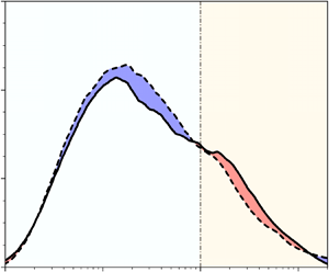
Figure 4. Comparison of the contribution  ${k_x\varPhi _{C_{f2}}}/{C_f}$ of physical length scales to
  $\langle \tau _w \rangle$ between OCF and CCF cases at
  ${\textit {Re}}_\tau =550$ (a) and 1000 (b), where the solid and dashed lines represent OCF and CCF cases, respectively. Red and blue shaded regions indicate the higher and lower value regions in OCF, respectively. Noting that both CCFDNS550 and CCFDNS550VL cases are shown in (a) for demonstrating the potential streamwise domain size effect, and the blue and red shaded regions correspond to the comparison between OCFDNS550 and CCFDNS550VL cases.
Though the curve shapes are generally similar, differences between the OCF and CCF curves can still be observed in figure 4(a). In the wavelength range of  $\lambda _x>O(10h)$ (roughly corresponding to the typical wavelength of VLSMs), the
  ${k_x\varPhi _{C_{f2}}}/{C_f}$ value in OCF is higher than that in CCF, indicating higher contributions of turbulent motions to
  $\langle \tau _w \rangle$ in the corresponding wavelength range in OCF. While in the wavelength range of
  $\lambda _x < O(10h)$, the
  ${k_x\varPhi _{C_{f2}}}/{C_f}$ value in OCF is lower than that in CCF. Almost identical curves observed for CCFDNS550 and CCFDNS550VL cases give a verification that the domain size of
  $8{\rm \pi} h \approx 25h$ is long enough to yield accurate results, based on which the results of OCFDNS550 case based on a domain size of
  $12{\rm \pi} h \approx 38h$ are also expected to be accurate enough. Accordingly, these observed differences of
  ${k_x\varPhi _{C_{f2}}}/{C_f}$ between OCF and CCF can be regarded as physical facts, rather than the limited streamwise domain size induced artefacts.
Figure 4(b) further presents the comparison of  ${k_x\varPhi _{C_{f2}}}/{C_f}$ between OCF and CCF at
  ${\textit {Re}}_\tau =1000$ (experimental OCF1000 and CCF1000 cases). Noting that
  ${k_x\varPhi _{C_{f2}}}/{C_f}$ shown in figure 4(b) is estimated from the data within
  $75\leq y^{+}\leq {\textit {Re}}_\tau$, for both OCF1000 and CCF1000 cases, because the CCF1000 case data are limited within this
  $y$ range. Such an estimation of
  ${k_x\varPhi _{C_{f2}}}/{C_f}$ is sufficient accurate (the total area below the curve equals to 0.95
 $({C_{f2}}/{C_f})$, meaning that 95 % of the real value (
 $C_{f2}/C_f$) has been captured) to allow a reliable comparison of
  ${k_x\varPhi _{C_{f2}}}/{C_f}$ between OCF and CCF. Similar differences observed in both figures 4(a) and 4(b) give further supports that the observed differences of
  ${k_x\varPhi _{C_{f2}}}/{C_f}$ between OCF and CCF, namely higher and lower values in
  $\lambda _x>O(10h)$ and
  $\lambda_x < O(10h)$ range of OCF, are indeed physical.
These observed differences of  ${k_x\varPhi _{C_{f2}}}/{C_f}$ between OCF and CCF can be preliminarily clarified by checking the difference in the spectrum (
 $u$,
$u$,  $v$, and
  $uv$).
The premultiplied  $u$ and
  $v$ spectra, and
  $uv$ cospectra at multiple
  $y$ positions are compared between OCF and CCF at comparable Reynolds numbers in figure 5. The DNS cases at
  ${\textit {Re}}_\tau =550$ (OCFDNS550 and CCFDNS550VL) are first presented in figure 5(a), where the
  $u$ spectra,
  $v$ spectra and
  $uv$ cospectra are shown in columns (ii) to (iv), respectively, with the solid and dashed lines indicating OCF and CCF, respectively. As seen in figure 4, the regions between the curves are coloured for a better demonstration of the differences. To facilitate explanation, the profiles of turbulence intensities and Reynolds shear stress are presented in the leftmost column (i), where the solid and dashed lines again indicate OCF and CCF, respectively, and different statistical quantities are distinguished by colour.

Figure 5. Comparison of the statistical quantities and spectra between OCF and CCF at comparable Reynolds numbers, where column (i) presents the profiles of statistical quantities, and columns (ii) to (iv) show the  $u$ spectra,
  $v$ spectra and
  $uv$ cospectra at typical
  $y$ positions respectively, with the positions marked by horizontal grey dashed arrows in column (i). Comparisons are made at
  ${\textit {Re}}_\tau =550$, 1000, and 1500 in (a), (b), and (c) respectively: (a) OCFDNS550 and CCFDNS550VL; (b) OCF1000 and CCF1000; (c) OCF1500 and CCF1600. In (b,c), since the statistical quantities for CCF1000 and CCF1600 cases are only available at discrete positions, the profiles of CCF DNS cases (CCFDNS1000 and CCFDNS2000) are presented additionally for verifying the accuracy of the experimental CCF cases; while in column (ii) to (iv) where the spectra are presented, the CCF spectra indeed refer to the experimental CCF1000 and CCF1600 cases rather than the DNS cases.
Comparisons of the turbulent quantities (column (i) of figure 5a) again reveal the long documented unique feature of turbulent kinetic energy (TKE) redistribution in the near free surface region of OCF (Komori et al. Reference Komori, Nagaosa, Murakami, Chiba, Ishii and Kuwahara1993; Nezu & Nakagawa Reference Nezu and Nakagawa1993; Zhong et al. Reference Zhong, Li, Chen and Wang2015), i.e. the wall-normal turbulence intensity is weakened while the streamwise one is enhanced. Since the turbulence intensities result from a superposition of various scales of turbulent motions, the differences in turbulence intensities indicate the presence of differences in turbulent motions. To reveal these expected differences, the (co)spectra at typical  $y$ positions (
 $y/h=0.2$, 0.5, 0.8, 0.95, as marked in column (i) of figure 5a) are shown in columns (ii) to (iv) of figure 5(a), where the spectral curves at different
  $y$ locations are shown from bottom to top with appropriate upward offsets on each higher
  $y$ position line. To make the differences of
  $uv$ cospectra between OCF and CCF more readable, the
  $uv$ cospectra at the last two higher
  $y$ positions are multiplied by a constant (as marked in column (iv)).
Let's first focus on the  $u$ spectra (column (ii) of figure 5a). As expected, in the near-wall positions (e.g.
  $y/h=0.2$), the curves of OCF and CCF are roughly the same. While moving away from the wall, the area under the OCF curve becomes greater than that of CCF because of higher streamwise turbulence intensity in OCF. By checking the wavelength, it can be seen that the extra area is mainly contributed from VLSMs. These observed differences of the premultiplied
  $u$ spectra between OCF and CCF are well consistent with the authors’ recent findings (Duan et al. Reference Duan, Chen, Li and Zhong2020a), and both demonstrate that VLSMs in OCF are stronger than those in CCF. Then we could know that in the wavelength range of
  $\lambda _x>O(10h)$ (roughly corresponding to the typical wavelength of VLSMs), the turbulent motions in OCF are stronger than those in CCF.
The  $v$ spectra (column (iii) of 5a), unlike the
  $u$ spectra where the large scale turbulent motions (LSMs and VLSMs) play important roles, indicate that the dominant motions are mainly small scale motions (with the peak energy located at
  $\lambda_x < h$). Near the wall, the curves for OCF and CCF coincide well. While when approaching the free surface, the OCF curve becomes lower than that of CCF (see e.g. the curves at
  $y/h=0.8$ and 0.95); this is reasonable because the wall-normal turbulence intensity in OCF is lower therein. Besides this magnitude difference, another noticeable difference lies in the shift of the peak (which indicates the most dominant motions) towards smaller scales in OCF when approaching the free surface.
The difference of  $uv$ cospectra between OCF and CCF is shown in column (iv) of figure 5(a). It is clear that OCF exceeds CCF in
  $\lambda _x>O(10h)$ range; in the
  $\lambda_x < O(10h)$ range, however, CCF turns to exceed OCF. From the comparisons of
  $u$ and
  $v$ spectra, it can be known that higher and lower
  $uv$ cospectra in the two
  $\lambda _x$ ranges of OCF are mainly contributed by the higher contribution of VLSMs revealed in
  $u$ spectra, and lower contribution of smaller scales revealed in
  $v$ spectra.
One main concern in the comparison of OCFDNS550 and CCFDNS550VL (figure 5a) is the low Reynolds number. To address such concern, similar comparisons were further performed for higher Reynolds number experimental cases, i.e. OCF1000 and CCF1000 (see figure 5b), and OCF1500 and CCF1600 (see figure 5c). In column (i) of figures 5(b) and 5(c) where statistical quantities are presented, we also included the CCF DNS cases (CCFDNS1000 and CCFDNS2000) for comparison and checking the reliability of CCF experimental data, which are only available at several discrete  $y$ positions. While in column (ii) to (iv) where spectra are presented, the CCF spectra indeed refer to experimental cases rather than DNS cases. The raw measured
  $uv$ cospectra need to be rescaled to avoid the magnitude effect of the measured Reynolds shear stress on the comparison. This can be explained as follows: at a given position the Reynolds shear stress in theory
  $(-\langle uv\rangle )_{theory}$ should satisfy the theoretical equation
  $(-\langle uv\rangle )_{theory} +\nu ({\partial U}/{\partial y})=u_\tau ^{2}(1-{y}/{h})$. However, the measured one
  $(-\langle uv\rangle )_{measured}$ is generally not exactly equal to
  $(-\langle uv\rangle )_{theory}$. Given that the raw measured
  $uv$ cospectrum
  $(\varPhi _{uv})_{measured}$ is obtained by
  $(\langle uv\rangle )_{measured}=\int _{0}^{\infty }(\varPhi _{uv})_{measured}\,\mathrm {d}k_x$, the magnitude of
  $(-\langle uv\rangle )_{measured}$ would directly affect the magnitude of
  $(\varPhi _{uv})_{measured}$, and thus prevent reliable comparison of
  $uv$ cospectra if
  $(-\langle uv\rangle )_{measured}$ is not rescaled to equal the theoretical one
  $(-\langle uv\rangle )_{theory}$. Therefore, for both OCF and CCF,
  $uv$ cospectra are rescaled as
  $(\varPhi _{uv})_{measured}$
  ${(-\langle uv\rangle )_{theory}}/{(-\langle uv\rangle )_{measured}}$. It can be seen that similar differences between OCF and CCF observed in figure 5(a) also occur in figures 5(b) and 5(c), demonstrating that increase in Reynolds number exerts no observable influence on such differences.
Beyond the above phenomenal explanations using spectra, we would give some more physical explains. As known to us, in the region close to the outer boundary of OCF and CCF, the velocity gradient is very small and  $\nu ({\partial U}/{\partial y})$ is negligible. Then
  $-\langle uv\rangle$ approximately follows a linear variation
  $-\langle uv\rangle =u_\tau ^{2}(1-{y}/{h})$, and taking a derivative along
  $y$ direction yields
 \begin{equation} \frac{\partial \left\langle uv\right\rangle }{\partial y}=\left\langle u \frac{\partial v}{\partial y}\right\rangle +\left\langle v \frac{\partial u}{\partial y}\right\rangle =\frac{u_\tau^{2}}{h}, \end{equation}
which holds both for OCF and CCF. The only difference between OCF and CCF is the upper boundary, i.e. a free surface presents in OCF, which affects the underlying turbulence by both dynamic and kinematic boundary conditions. The former one requires zero tangential stresses at the free surface and causes the surface layer which is a thin region adjacent to the free surface characterized by fast variations of the horizontal vorticity, while the latter one requires no mass flux at the free surface and produces the blockage layer within which TKE redistribution phenomena are observed. According to a recent DNS study from Bauer (Reference Bauer2015), the blockage layer thickness was demonstrated to scale in outer units ( $\sim$0.3
 $h$).
$h$).
Ideally, if the free surface in OCF is flat without fluctuations, the wall-normal velocity at the free surface is exactly zero and (3.1) can be written as
 \begin{equation} \left.\frac{\partial \left\langle uv\right\rangle }{\partial y}\right|_{y=h} = \left\langle u \frac{\partial v}{\partial y}\right\rangle.\end{equation}
By further invoking the continuity equation, (3.2) can be rewritten as
 \begin{equation} \left.\frac{\partial \left\langle uv\right\rangle }{\partial y}\right|_{y=h} = \left\langle u \frac{\partial v}{\partial y}\right\rangle ={-}\left\langle u \left(\frac{\partial u}{\partial x}+ \frac{\partial w}{\partial z} \right) \right\rangle ={-}\left\langle \frac{1}{2}\frac{\partial u^{2}}{\partial x}\right\rangle- \left\langle u\frac{\partial w}{\partial z}\right\rangle. \end{equation}
 At steady and uniform conditions, the flow is homogenous along  $x$ direction and the mean value of the derivative of any flow quantities in terms of
  $x$ would be zero. Then we could have
 \begin{equation} \left.\frac{\partial \left\langle uv\right\rangle }{\partial y}\right|_{y=h} = \left\langle u \frac{\partial v}{\partial y}\right\rangle ={-}\left\langle u\frac{\partial w}{\partial z}\ \right\rangle = \frac{u_\tau^{2}}{h} >0,\end{equation}
based on which it can be known that in the near free surface region the fluctuating velocity components statistically satisfy the following relations:
 \begin{equation} \left.\begin{array}{ll@{}} \displaystyle \dfrac{\partial v}{\partial y} >0 \quad \mathrm{and}\quad \dfrac{\partial w}{\partial z} <0,\quad \mathrm{when}\ u>0 \\ \displaystyle \dfrac{\partial v}{\partial y} <0 \quad \mathrm{and}\quad \dfrac{\partial w}{\partial z} >0,\quad \mathrm{when}\ u<0 \end{array}\right\}.\end{equation}
 The streamwise rotating motions satisfy (3.5) and can be explained by figure 6(a), where a pair of streamwise rotating motions is presented for demonstration. On the upwelling rotation sides, low momentum fluids are pumped up to the free surface, leading to  $u<0$ (see regions marked in blue). Accordingly,
  $v$ and
  $w$ gradually decrease and increase, respectively, when approaching the free surface, meaning that
  $\partial v/\partial y<0$ and
  $\partial w/\partial z>0$ on upwelling sides. While on the downwelling sides, the high momentum fluids at the free surface are pumped downwards to the wall, leading to
  $u>0$ (see regions marked in red),
  $\partial v/\partial y>0$ and
  $\partial w/\partial z<0$. Analogically, for streamwise rotating motions with opposite rotation directions, the same relationships can be derived. As can be seen, all the flow features of streamwise rotating motions satisfy the derived relations in (3.5).

Figure 6. Schematic demonstration of the turbulent motions in OCFs to explain the possible mechanisms for the observed differences of scale-dependent turbulent contributions to  $\langle \tau _w \rangle$ between OCF and CCF (i.e. higher and lower turbulent contribution in
  $\lambda _x>O(10h)$ and
  ${<}O(10h)$ range in OCF shown in figure 4.).
These streamwise rotation motions can develop into different sizes of streamwise vortices: when the vertical motions are weak and localized in the vicinity of the free-surface, the generated streamwise vortices are small in size and supposed to locally reside in the near free-surface region; while when the vertical motions are strong enough to penetrate the whole water depth (e.g. whole water depth ejections/sweeps), water-depth scaled streamwise vortices can be generated (see figure 6c) and have been well documented in the literature with different terminologies, e.g. super-streamwise vortices, roll cells, etc. (Adrian & Marusic Reference Adrian and Marusic2012; Zhong et al. Reference Zhong, Li, Chen and Wang2015, Reference Zhong, Chen, Wang, Li and Wang2016). Although these streamwise vortices also persist near the outer boundary of CCFs, they are speculated to be less populated and weaker due to the absence of upper boundary restrictions on vertical motions, which can be readily seen from the much higher wall-normal turbulence intensity near the upper boundary of CCFs than that of OCFs (see column (i) of figure 5).
Above analysis focuses on the upper boundary (free surface) related motions. Now we would discuss the lower boundary (solid wall) related motions, specifically the wall-attached ones that are relevant to wall-shear stresses studied herein. The earliest work can date back to Townsend's attached eddy hypothesis (Townsend Reference Townsend1976), where double-cone vortices were adopted as representative wall-attached motions, whose signatures in  $yz$ plane are counter-rotating streamwise vortices (as depicted in figure 6b). With better understandings of turbulent motions, it has been known that the representative wall-attached motions can be refined by hairpin packets (Marusic & Monty Reference Marusic and Monty2019), i.e. the transportation roles of hairpin packets give rise to these counter-rotating streamwise vortices. The wall-attached motions are geometrically self-similar in the log region with their scales proportional to the distance to the wall
  $y$. In
  $yz$ plane, their diameters are roughly equal to
  $y$ (figure 6b). In
  $xy$ plane, Baars, Hutchins & Marusic (Reference Baars, Hutchins and Marusic2017) and Duan et al. (Reference Duan, Zhang, Zhong, Zhu and Li2020b) demonstrated that the streamwise wavelength of wall-attached motions in TBL and OCF follows a linear variation with
  $y$ as
  $\lambda _x=14y$ up to
  $y/h=0.7$ (where
  $\lambda _x=10h$). Beyond
  $y/h=0.7$, the streamwise wavelength increases more dramatically and reaches
  $\lambda _x\sim 20h$ at the free-surface in OCF (Duan et al. Reference Duan, Zhang, Zhong, Zhu and Li2020b) (as schematically shown in figure 6d). Since
  $\lambda _x$ indicates a whole cycle of positive and negative velocity fluctuations, wall-attached motions represented by
  $\lambda _x$ could be depicted as a whole cycle of sweeps and ejections in
  $xy$ plane whose streamwise extend equals
  $\lambda _x$ (see figure 6e).
Finally, based on the above discussions on the free-surface and wall related motions in OCFs, we could have a sound physical explanation on the observed differences of scale-dependent turbulent contributions to  $\langle \tau _w \rangle$ between OCF and CCF (i.e. higher and lower turbulent contribution in
  $\lambda _x>O(10h)$ and
  ${<}O(10h)$ range in OCF, as shown in figure 4): the streamwise wavelength of wall-attached motions in the near free surface blockage layer (
 $y/h>0.7$) reaches a value of
  $\lambda _x>10h$. Such scale of wall-attached motions will interact with the free surface. The essential roles of the free surface in generating/promoting near-surface or whole water depth streamwise vortices would enhance the strength of these wall-attached motions whose spatial signatures are also streamwise vortices. Then these enhanced wall-attached motions with
  $\lambda _x>10h$ would exert a stronger effect on the wall, thus leading to higher turbulent contributions to
  $\langle \tau _w \rangle$ in the
  $\lambda _x>O(10h)$ range of OCF, when compared to CCF. Given the total turbulent contributions are identical between OCF and CCF, higher contributions in the
  $\lambda _x>O(10h)$ range necessitate lower contributions in the
  $\lambda _x < O(10h)$ range.
3.4. Contributions from different scale ranges
For practical purpose, besides the scale-by-scale contributions, it is also desirable to know the contributions in a sense of scale range, i.e. the fractions of  $\langle \tau _w \rangle$ contributed from a specific scale range of turbulent motions.
Figure 7 first shows the cumulative turbulent contribution profile  ${Cum}_{turb}(\lambda _x)$ (corresponding to an integration of the area below the
  ${k_x\varPhi _{C_{f2}}}/{C_f}$ curve), where
  ${Cum}_{turb}(\lambda _x)$ value at a specific wavelength indicates the total turbulent contributions from all scales of turbulent motions smaller than this given wavelength. Compared to
  ${Cum}_{turb}(y)$ shown in figure 1 which is an indication of the cumulative turbulent contribution to
  $\langle \tau _w \rangle$ vs
  $y$,
$y$,  ${Cum}_{turb}(\lambda _x)$ shown in figure 7 indicates the cumulative turbulent contribution to
  $\langle \tau _w \rangle$ vs wavelength
  $\lambda _x$. Again, it should be mentioned here that since only the turbulent contribution portion is considered,
  ${Cum}_{turb}$ will not attain the value 100 % but
  $C_{f2}/C_f$ at the largest wavelength.

Figure 7. Cumulative turbulent contribution of physical length scales to  $\langle \tau _w \rangle$,
  ${Cum}_{turb} (\lambda _x)$, where inner- and outer-scale normalized wavelengths are used in (a) and (b), respectively.
Inner- and outer-scale normalized wavelengths are used in figures 7(a) and 7(b), respectively. As can be seen from figure 7(a), when the curves are represented as a function of inner-scale normalized wavelength  $\lambda _x^{+}$, an obvious Reynolds number dependence of the curves can be observed, where the cumulative contribution value at a given
  $\lambda _x^{+}$ decreases as the Reynolds number increases. When the curves are represented as a function of outer-scale normalized wavelength
  $\lambda _x/h$ (see figure 7b), though a minor Reynolds number dependence can still be observed, the curves at different Reynolds numbers generally agree well with each other.
By specifying appropriate cut-off wavelength ranges in figure 7, the contributions from specified scale range can be obtained. Motivated by the significant roles of VLSMs in contributing to the turbulent kinetic energy and Reynolds shear stress (carrying over 50 % of the kinetic energy and Reynolds shear stress (Guala et al. Reference Guala, Hommema and Adrian2006; Balakumar & Adrian Reference Balakumar and Adrian2007; Duan et al. Reference Duan, Chen, Li and Zhong2020a), we first adopted the most classical dividing wavelength  $\lambda _x=3h$ between LSMs and VLSMs to see the fractions of
  $\langle \tau _w \rangle$ contributed by VLSMs. Such results are presented in figures 8(a) and 8(b), where the results of present OCFs are shown in figure 8(a), and comparisons between OCF and CCF at
  ${\textit {Re}}_\tau =550$ (i.e. OCFDNS550 and CCFDNS550VL) are presented in figure 8(b). For the sake of completeness, the remaining contribution components (the laminar contribution, and contribution from
  $\lambda_x < 3h$) are also included. It can be seen that the VLSMs (with a wavelength
  $\lambda _x>3h$) contribute over 40 %, while the turbulent motions with wavelength
  $\lambda_x < 3h$ contribute about 50 % of
  $\langle \tau _w \rangle$ in OCFs. Compared to CCF, slightly higher and lower contribution values in
  $\lambda _x>3h$ and
  ${<}3h$ range are observed in OCF (see figure 8b), which is expected according to the observations in the previous subsection.

Figure 8. Contributions of different scale ranges of turbulent motions to  $\langle \tau _w \rangle$ by adopting cut-off wavelengths of
  $\lambda _x=3h$ (a,b) and
  $10h$ (c,d). (a,c) Results of present OCF cases at different Reynolds numbers. (b,d) Comparisons between OCF and CCF at
  ${\textit {Re}}_\tau =550$.
Further results are obtained by adopting a larger dividing wavelength of  $\lambda _x=10h$ (approximately corresponding to the dividing wavelength that OCF and CCF exhibit differences in the turbulent contributions to
  $\langle \tau _w \rangle$, see figure 4), and the results are presented in figures 8(c) and 8(d). As can be seen in figure 8(c), the turbulent motions with
  $\lambda _x>10h$ contribute over 20 % of
  $\langle \tau _w\rangle$, while the turbulent motions with
  $\lambda_x < 10h$ make a contribution of about 70 % in the present OCFs. The differences in the contributions from different scale ranges between OCF and CCF are again revealed in figure 8(d).
Finally, it is worth mentioning here that although the application of Taylor's hypothesis in the experimental cases (OCF1000 to OCF2400) would exert some effects on the curve shapes of  ${Cum}_{turb}$ in figure 7 and thus affect the exact contribution values in different scale ranges as shown in figure 8, such effects would not affect the main findings in figure 8 that turbulent motions with
  $\lambda _x>3h$ contribute over 40 % of
  $\langle \tau _w\rangle$, and turbulent motions with
  $\lambda _x>10h$ contribute over 20 % of
  $\langle \tau _w\rangle$. This statement is mainly supported by the OCFDNS550 case combined with the Reynolds number dependence trends, i.e. the contribution values (40 % for
  $\lambda _x>3h$ and 20 % for
  $\lambda _x>10h$) obtained in OCFDNS550 case are the lower bounds given that the contributions of these large scale turbulent motions to
  $\langle \tau _w \rangle$ increase as the Reynolds number increases. Therefore, it is safe to conclude here that the VLSMs with
  $\lambda _x>3h$ contribute over 40 % of
  $\langle \tau _w \rangle$, and turbulent motions with
  $\lambda _x>10h$ contribute over 20 % of
  $\langle \tau _w \rangle$ in OCFs within the Reynolds number range considered here (
 ${\textit {Re}}_\tau$ from a low of 550 to a moderate value of 2400).
4. Conclusions
Contributions of different scales of turbulent motions to the mean wall-shear stress  $\langle \tau _w \rangle$ in OCFs were quantified based on the FIK identity decomposition method combined with a scale decomposition. The OCF datasets considered herein covered both DNS and PIV experimental cases with the friction Reynolds number
  ${\textit {Re}}_\tau$ ranging from a low of 550 to a moderate value of 2400. Comparisons of the results between OCF and CCF were also performed to reveal potential differences between the two flow configurations. The main findings can be summarized as follows.
(1) Both the ‘laminar’ and ‘turbulent’ components of
 $\langle \tau _w \rangle$ in OCFs have been shown to be identical to those in CCFs at identical Reynolds numbers, demonstrating the commonality of the two flow types.
(2) The scale-decomposed ‘turbulent’ contribution shows two dominant contribution modes (corresponding to LSMs and VLSMs) at a streamwise wavelength of
$\lambda _x=1\sim 2h$ and $O(10h)$. As the Reynolds number increases, the contributions from the two modes (LSMs and VLSMs) gradually decrease and increase respectively, indicating the enhanced significance of VLSMs in contributing to $\langle \tau _w \rangle$ at higher Reynolds numbers. Within the Reynolds number range considered, the VLSMs with $\lambda _x>3h$ account for over 40 % of $\langle \tau _w \rangle$ and turbulent motions with $\lambda _x>10h$ account for over 20 % of $\langle \tau _w \rangle$.(3) Comparisons of the scale-decomposed ‘turbulent’ contribution between OCF and CCF have revealed scale-dependent differences. Compared to CCFs, higher and lower contributions in
$\lambda _x>O(10h)$ and $\lambda_x < O(10h)$ wavelength ranges are observed in OCFs. Given that the only difference between the two flows is the outer boundary, i.e. a free surface exists in OCFs, the above differences indicate important free surface effects on the turbulent contributions to $\langle \tau _w \rangle$ in OCFs.


Acknowledgements
We express our sincere gratitude to: Professor D.H. Richter (University of Notre Dame) for sharing the OCF DNS data at  ${\textit {Re}}_\tau =550$; Dr R. Deshpande, Professor J.P. Monty, and I. Marusic (University of Melbourne) for sharing the CCF experimental data at
  ${\textit {Re}}_\tau =1000$; Dr A. Lozano-Durán (Stanford University) and Professor J. Jiménez (Universidad Politécnica Madrid) for sharing the very large domain size CCF DNS data at
  ${\textit {Re}}_\tau =550$; Professor M. Lee and R.D. Moser (The University of Texas at Austin) for making the CCF DNS database publicly available.
Funding
The study was financially supported by the National Natural Science Foundation of China (grant nos 51879138 and 51809268) and the Joint Fund of State Key Lab of Hydroscience and Institute of Internet of Waters Tsinghua-Ningxia Yinchuan (grant no. sklhse-2020-Iow06).
Declaration of interests
The authors report no conflict of interest.
Appendix A. Data accuracy verification
A.1. Statistical quantities
Typical turbulent statistical quantities for present OCF cases are first presented in figure 9 to give a preliminary data accuracy verification. For comparison, the results of comparable CCF cases and theoretical formulas (e.g. log law for mean streamwise velocity, linear distribution of Reynolds shear stress in the outer region, and empirical functions for turbulence intensities proposed by Nezu & Rodi Reference Nezu and Rodi1986) are also included. As seen in figure 9, there exists good agreement in the distribution of all turbulent quantities. The discrepancy in turbulence intensity between OCF and CCF in the nearly free surface region demonstrates the well-documented unique features of turbulent kinetic energy (TKE) redistribution in OCFs, i.e. the free surface dampens the wall-normal turbulence intensity but strengthens the wall-parallel ones.

Figure 9. Wall-normal profiles of inner-scale normalized statistical quantities: (a) mean streamwise velocity; (b) turbulence intensities and Reynolds shear stress (here negative valued Reynolds shear stress is shown for a better demonstration purpose). The black line and symbols are present open channel flow (OCF) cases, and the remaining lines and symbols in color are these of closed channel flows (CCFs) and empirical functions for comparison. For the log law in (a), von Kármán constant  $\kappa =0.412$ and additive constant
  $A=5.29$ are used (Nezu & Nakagawa Reference Nezu and Nakagawa1993). The green lines and expressions in (b) indicate the classical functions for given quantities, among which the functions for the turbulence intensities are from Nezu & Rodi (Reference Nezu and Rodi1986).
A.2. The $uv$ cospectra and uncertainties

Since the  $uv$ cospectrum
  $\varPhi _{uv}$ is most essential to the scale decomposition of the mean wall-shear stress, its estimation method and accuracy should also be discussed herein. For the OCF DNS case (OCFDNS550),
  $\varPhi _{uv}$ at a given
  $y$ position was directly obtained from the spatial velocity data according to (2.2), among which the ensemble average was performed over spanwise positions and snapshots. For the experimental OCF flow cases,
  $\varPhi _{uv}$ was obtained from the temporal velocity data using Welch's overlapped segment averaging method. The segment length was chosen to be long enough to ensure the largest wavelength resolved at all
  $y$ positions is over
  $100h$. A segment overlap percentage of 50 % was adopted, based on which the segment number
  $N_{seg}$ for the five cases (OCF600 to OCF2400) is
  $122\sim 204$. To avoid spectral leakage at the segment edge, a hamming window was applied on each segment before performing the Fourier transform as advocated by Buxton, de Kat & Ganapathisubramani (Reference Buxton, de Kat and Ganapathisubramani2013). Given that the raw spectrum obtained from the raw velocity data would be inherently contaminated by the high-frequency measurement noise, a 9-point Gaussian kernel with a standard deviation of 1.7 was applied to the raw velocity data to reduce noise effects. And a bandwidth moving filter (BMF) (Baars et al. Reference Baars, Hutchins and Marusic2016) of 25 % (meaning that the filtered spectrum at wavenumber
  $k_{xi}$ equals an average of the raw spectrum over a span of
  $k_{xi}\pm 25\,\%$) was further adopted to smooth the spectrum. One of main concerns on the experimental spectra is the use of Taylor's hypothesis for frequency
  $f$ to wavenumber
  $k_x$ transformation:
  $k_x={2{\rm \pi} f}/{U_c}$. As the only parameter in Taylor's hypothesis, the convection velocity
  $U_c$ should depend on the localized motion scales and events (del Álamo & Jiménez Reference del Álamo and Jiménez2009; de Kat & Ganapathisubramani Reference de Kat and Ganapathisubramani2015; Renard & Deck Reference Renard and Deck2015; Fiscaletti, de Kat & Ganapathisubramani Reference Fiscaletti, de Kat and Ganapathisubramani2018) in theory, but complete expression of
  $U_c$ with them is generally inaccessible in applications, given which a scale- and event-independent convection velocity is typically adopted for application purpose. Actually, in most cases where Taylor's hypothesis has been applied (e.g. the widely used single point HWA measurements in abundant studies, including the CCF1000 (Deshpande et al. Reference Deshpande, Monty and Marusic2020) and CCF1600 (Balakumar Reference Balakumar2005; Balakumar & Adrian Reference Balakumar and Adrian2007) experimental cases considered herein), the local mean velocity
  $U$ was the only accessible choice. Abundant studies have demonstrated that
  $U$ is a good surrogate of
  $U_c$ that could give sufficient accurate spectra results, except in the near-wall region (de Kat & Ganapathisubramani Reference de Kat and Ganapathisubramani2015; Squire et al. Reference Squire, Hutchins, Morrill-Winter, Schultz, Klewicki and Marusic2017, to name a few). In this study, for the convenience of comparison between the experimental OCF and CCF cases, we would mainly confine our estimations of the spectra through Taylor's hypothesis using the local mean velocity
  $U$. This would only exert minor effects on the main findings of this study, which has been discussed in § 3.
Figure 10 presents the resultant cospectra at a typical position ( $y/h=0.2$) to give a primary accuracy verification. The results of CCF cases at identical positions are also included for comparison. The high-frequency measurement noise can be readily seen at high wavenumber range of the raw unfiltered spectrum. The filtering procedures adopted herein effectively reduced this high-frequency noise and also the inherent fluctuations of the raw spectrum. A conservative estimation of the smallest scales that can be resolved at this position is
  $\lambda _x=0.16h$ and
  $0.07h$, or equivalently
  $\lambda _x^{+}=100$ and
  $170$, for the lowest and highest
  ${\textit {Re}}_\tau$, respectively. Good agreements observed between experiments and DNS, as well as between OCF and CCF cases, lend supports for the data accuracy and the rationality of processing procedures.

Figure 10. The  $uv$ cospectra
  $\varPhi _{uv}$ at
  $y/h=0.2$. The solid lines are present OCF results, among which the experimental ones are obtained from the Gaussian filtered velocity data followed by 25 % BMF filtering. As references, the raw unfiltered results obtained from the raw velocity data are also presented (as marked by an arrow in the figure). For comparison, the results of CCF cases at identical positions are also included.
Finally, the cospectra uncertainty will be briefly presented. Treating the spectrum estimation from each segment as a random quantity denoted as  $\phi _{uv}$ whose ensemble average is the cospectra
  $\varPhi _{uv}$, the uncertainty of
  $\varPhi _{uv}$ can be quantified according to the general uncertainty quantification method (Sciacchitano & Wieneke Reference Sciacchitano and Wieneke2016) as
  $\delta \varPhi _{uv}={\sigma _{\phi _{uv}}}/{\sqrt {N_{eff}}}$. Here
  $\sigma _{\phi _{uv}}$ is the standard deviation of
  $\phi _{uv}$ and
  $N_{eff}$ is the effective number of independent samples and can be replaced with the segment number
  $N_{seg}$ herein. The uncertainty of DNS cases is generally expected to be negligible. Here we would put our emphasis on the experimental cases, for which
  $\delta \varPhi _{uv}$ is estimated to be mainly at a level of
  $\sim$10 %
  $\varPhi _{uv}$, except in the near free surface region where
  $\varPhi _{uv}$ is tending to zero (because
  $\langle uv \rangle$ is approaching zero therein) and for which reason the uncertainty
  $\delta \varPhi _{uv}$ expressed as a percentage of
  $\varPhi _{uv}$ would be higher.


