


1. Introduction
Fluid flows past multiple structures that are long in a direction perpendicular to the flow, but with a bluff or non-aerodynamic cross-section – such as cylinders – abound in engineering and nature. From the vibration of high-voltage power lines in cross winds (Tsui Reference Tsui1986) and the cooling of nuclear fuel rods (Lee & Choi Reference Lee and Choi2007), to the mass transport through aquatic vegetation (Nepf Reference Nepf2012) and even the sensing capacity of harbour seal vibrissae or whiskers (Hanke et al. Reference Hanke, Witte, Miersch, Brede and Oeffner2010), understanding the vortex formation in such flows is vital to their control, manipulation and exploitation.
The canonical system in this class is the flow past two identical circular cylinders. This problem is defined by two parameters, the Reynolds number  $Re = UD/\nu$ and the normalised distance between the cylinder centres or pitch
  $p = x_c/D$, where
  $U$ is the free-stream velocity,
  $D$ is the diameter of the cylinders,
  $\nu$ is the kinematic viscosity and
  $x_c$ is the distance between the cylinder centres.
For values of pitch  $p \lesssim 3.6$, the separated shear layers from the front cylinder reattach to the rear cylinder, and the two bodies behave as a single, streamlined body with periodic vortex shedding in its wake at a single distinct frequency. However, for longer pitch, the shear layers from the front cylinder roll up into distinct vortices, and periodic vortex shedding similar to that seen from a single isolated cylinder occurs in the gap between the cylinders, and these vortices then impinge on the rear cylinder. As a result of this interaction, a two-row structure of vortex shedding appears behind the second cylinder. This process, and the critical value of pitch
  $p$ at which vortex shedding in the gap occurs, has been shown to be only weakly affected by the Reynolds number over the range
  $200 \leqslant Re < 10^5$ (Zdravkovich Reference Zdravkovich1987; Sumner, Price & Paidoussis Reference Sumner, Price and Paidoussis2000; Hu & Zhou Reference Hu and Zhou2008; Sumner Reference Sumner2010; Zhou & Alam Reference Zhou and Alam2016; Griffith et al. Reference Griffith, Lo Jacono, Sheridan and Leontini2017).
The purpose of this paper is to demonstrate two distinct phenomena related to this two-row structure. The first is that this structure does not share the feedback characteristics of the wake of a single cylinder. In fact, subsequent bodies can be placed anywhere over a large range of lengths, which we quantify below, with essentially no impact on the flow both upstream and downstream. Subsequent bodies are cloaked – their presence is not communicated to the flow or to other bodies in the array and the mean drag on these bodies has a very small value. The second phenomenon, in stark contrast to the first, is that even small disturbances introduced in a region that is close, but not directly adjacent, to the second cylinder trigger a global change in the flow, destroying the two-row structure and completely suppressing the vortex shedding from the first cylinder. Here, subsequent bodies are broadcast – their presence is signalled throughout the flow.
We analyse this behaviour using two techniques. First, we use a local stability analysis to try to understand the broadcasting phenomenon in terms of the transport of perturbations introduced by the presence of the third body. The majority of the two-row structure is reminiscent of two free shear layers that are harmonically forced – such shear layers produce trains of vortical structures at the same frequency as the forcing and are known to be convectively unstable (Browand Reference Browand1966; Brown & Roshko Reference Brown and Roshko1974; Monkewitz & Huerre Reference Monkewitz and Huerre1982; Ho & Huerre Reference Ho and Huerre1984; Huerre & Monkewitz Reference Huerre and Monkewitz1985; Ghoniem & Ng Reference Ghoniem and Ng1987). Our analysis shows that the majority of the mean flow of the two-row structure is marginally convectively unstable, except for a small region that is weakly absolutely unstable close to the second body. While such a simplified analysis cannot be considered predictive, this finding suggests that there should be an upper limit on the downstream distance of the position of a third body that can trigger a global change. As perturbations introduced by the presence of a third body in a convectively unstable region should be swept downstream and not communicated upstream, the onset of convective instability should indicate the end of the potential to trigger a global change in the flow. This coincides with the end of the potential to broadcast the presence of the third body. We confirm the phenomenological prediction of the presence of an upper limit from the local analysis performed on the wake of the two-cylinder system by manually placing subsequent third bodies of varying shape in the wake. The threshold location for the most upstream point of the third body that delineates the positions that trigger the broadcasting or cloaking behaviour coincides closely with the transition point from the absolutely unstable region to the convectively unstable region. However, an upper and lower boundary for the body position that can trigger a global change (i.e. the broadcasting phenomenon) is found using simulation, and the lower boundary is not predicted with the local stability analysis as the absolutely unstable region extends all the way upstream to the rear of the second cylinder.
We therefore introduce an adjoint-based sensitivity analysis to assess the sensitivity of the time-mean wake of the two-cylinder system (Giannetti & Luchini Reference Giannetti and Luchini2007; Luchini & Bottaro Reference Luchini and Bottaro2014; Meliga et al. Reference Meliga, Boujo, Pujals and Gallaire2014). A direct interpretation of the sensitivity field confirms the presence of an upper limit on the body position, but it fails to predict the presence of the lower boundary. However, we present an argument that shows that the third cylinder cannot be treated as a small perturbation of the two-cylinder system, and the nonlinear correction of the mean flow induced by the presence of the third cylinder generates this lower boundary. Further, we show that while linear methods fail to completely predict the transition and saturation process between two global states that occurs during broadcasting, global linear stability analysis of the saturated mean flows does recover the global flow structure and frequency.
2. Methodology
2.1. Direct numerical simulations
The sharp interface immersed boundary method is used to simulate the flows in two dimensions. The body surfaces are modelled by a set of finite elements immersed in an underlying Cartesian grid and the incompressible Navier–Stokes equations govern the motion of fluid:
 \begin{equation} \left. \begin{gathered} \frac{\partial {\boldsymbol{u}}}{\partial \tau} = - ({\boldsymbol{u}}\boldsymbol{\cdot}\boldsymbol{\nabla}){\boldsymbol{u}} - \boldsymbol{\nabla} P + \frac{1}{Re}\nabla ^2 {\boldsymbol{u}} + \boldsymbol{A}_b,\\ \boldsymbol{\nabla}\boldsymbol{\cdot}{\boldsymbol{u}}=0, \end{gathered}\right\} \end{equation}
where  ${\boldsymbol {u}}$ is the velocity field non-dimensionalised by the free-stream velocity
  $U$,
$U$,  $\tau = tU/D$ is time non-dimensionalised by the advective time scale,
  $P$ is the pressure field non-dimensionalised by
  $\rho U^2$ and
  $\boldsymbol {A}_b$ is a generic acceleration term that models the presence of an immersed boundary. A second-order central finite-difference scheme is used to spatially discretise these equations. Temporal integration is performed using a two-way time splitting scheme that results in a Poisson equation being formed that can be solved for the pressure correction.
The flow domain in the simulation extends at least  $15D$ upstream and laterally of the centre of the array, and at least
  $30D$ downstream. Boundary conditions on the fluid domain are an imposed free-stream velocity and zero pressure gradient on the boundaries upstream and transverse of the bodies, and a zero-gradient velocity condition and zero pressure at the outlet or downstream boundary. At the surface of the bodies, a no-slip velocity condition and zero pressure gradient are imposed. The Cartesian grid used on the fluid domain has 64 points across
  $D$ in the vicinity of the bodies, and the bodies are represented by 128 elements. The basic method closely follows that presented in Mittal et al. (Reference Mittal, Dong, Bozkurttas, Najjar, Vargas and von Loebbecke2008) and Seo & Mittal (Reference Seo and Mittal2011). Validation of the code for multiple body flows and further details of the actual implementation used here can be found in Griffith & Leontini (Reference Griffith and Leontini2017) and Griffith et al. (Reference Griffith, Lo Jacono, Sheridan and Leontini2017).
2.2. Local stability analysis
The analysis proceeds by treating the wake as a slowly varying parallel shear flow. A series of streamwise velocity profiles are extracted from the mean flow at a set of downstream distances and the linear stability of each profile is then assessed. The body of work treating cylinder wakes in this way is reviewed in Chomaz (Reference Chomaz2005), and there are many examples of applying this technique to the mean flow in bluff-body wakes – see Hammond & Redekopp (Reference Hammond and Redekopp1997), Pier (Reference Pier2002), Thiria & Weisfreid (Reference Thiria and Weisfreid2007), Khor et al. (Reference Khor, Sheridan, Thompson and Hourigan2008) and Leontini, Thompson & Hourigan (Reference Leontini, Thompson and Hourigan2010). The relevance of the mean flow to the dynamics of vortex wakes has also been explored in a global sense in Barkley (Reference Barkley2006) and Mantič-Lugo, Arratia & Gallaire (Reference Mantič-Lugo, Arratia and Gallaire2014).
Assuming viscosity plays only a secondary role in the instability and can be neglected, the stability problem reduces to solving the Rayleigh equation (Drazin & Reid Reference Drazin and Reid2004) defined as
 \begin{equation} (\boldsymbol{U}_x-c)\left(\frac{\mathrm{d}^2{\phi}}{\mathrm{d}y{^2}}-k^{2}\phi\right)-\frac{\mathrm{d}^{2}{\boldsymbol{U}_x}}{\mathrm{d}{y}^{2}}\phi=0, \end{equation}
where  $\boldsymbol {U}_x$ is the streamwise velocity profile extracted from the mean flow,
  $c$ is the complex wave speed,
  $k$ is the complex wavenumber and
  $\phi$ is the complex amplitude of the infinitesimal perturbation stream function applied to the base flow. A complex frequency can be defined as
  $\omega = kc$. A characteristic complex frequency
  ${\omega _c}$ for each profile can be found, which is the frequency associated with a group velocity of zero – this occurs at pinch points in the complex
  $k$ plane, which coincide with cusp points in the complex
  $\omega$ plane (Huerre & Rossi Reference Huerre and Rossi1998). The imaginary component of
  ${\omega _c}$ dictates whether an instability on a particular velocity profile is absolute or convective. If the imaginary component is positive, disturbances grow in place and oscillate with a frequency given by the real component of
  ${\omega _c}$ – this is a local absolute instability, and it has its own inherent dynamics with a preferred oscillation frequency at the real component of
  ${\omega _c}$. If the imaginary component is negative, disturbances do not grow in place and are instead ‘washed out’ of the flow, potentially growing as they flow downstream – this is a local convective instability, and such a region of flow responds to any external forcing at the frequency of the external forcing. The process of finding
  ${\omega _c}$ (or equivalently the cusp points in the complex frequency plane) is further explained in Kupfer, Bers & Ram (Reference Kupfer, Bers and Ram1987) and in the context of wake flows by Leontini et al. (Reference Leontini, Thompson and Hourigan2010).
We note that such a local, inviscid, linear analysis of the mean flow is unlikely to be quantitatively predictive. However, it can provide insight and a framework for understanding the flow behaviour from a phenomenological perspective.
2.3. Sensitivity analysis
Sensitivity, or structural stability, analysis is a method for determining which spatial regions of a flow are most sensitive to disturbance, or structural perturbation. Such a structural perturbation may be the introduction of some external forcing, or simply the introduction of another object in the flow. These sensitive regions are identified by assessing the behaviour of perturbations to the base flow state.
Evolution equations for perturbations are formed by decomposing the flow solution into base and perturbation components, substituting this into the equations of motion (2.1), subtracting base flow terms and linearising the result to arrive at
 \begin{equation} \left. \begin{gathered} \frac{\partial {\boldsymbol{u}^{{\prime}}}}{\partial \tau} = - \left[({\boldsymbol{U}}\boldsymbol{\cdot}\boldsymbol{\nabla}){\boldsymbol{u}^{{\prime}}} + ({\boldsymbol{u}^{{\prime}}}\boldsymbol{\cdot}\boldsymbol{\nabla}){\boldsymbol{U}}\right] - \boldsymbol{\nabla} {p^{\prime}} + \frac{1}{Re}\nabla^2 {\boldsymbol{u}^{{\prime}}} + \boldsymbol{A}^{\prime}_{b},\\ \boldsymbol{\nabla}\boldsymbol{\cdot}{\boldsymbol{u}^{{\prime}}}=0, \end{gathered}\right\} \end{equation}
where  ${\boldsymbol {U}}$ is the base flow velocity field,
  ${\boldsymbol {u}^{{\prime }}}$ and
  ${p^{\prime }}$ are the perturbation velocity and pressure fields, respectively, and
  $\boldsymbol {A}^{\prime }_{b}$ is the perturbation acceleration term introduced to account for the immersed bodies. Note the
  ${\boldsymbol {U}}$ is the base flow of which the sensitivity is being assessed.
Since (2.3) represents a linear operator it can be cast as
 \begin{equation} {\boldsymbol{u}^{{\prime}}}(t+T) = {\boldsymbol{\mathsf{L}}}{\boldsymbol{u}^{{\prime}}}(t). \end{equation}
Traditional linear stability analysis proceeds by solving for the eigenvectors and associated eigenvalues of  ${\boldsymbol{\mathsf{L}}}$ such that
 \begin{equation} {\boldsymbol{\mathsf{L}}}{\boldsymbol{u}^{{\prime}}}(t) = \mu{\boldsymbol{u}^{{\prime}}}(t). \end{equation}
If any eigenvector, or mode, of  ${\boldsymbol{\mathsf{L}}}$ has an associated eigenvalue or multiplier such that
  $|\mu | > 1$, then that mode is predicted to grow and the base flow
  ${\boldsymbol {U}}$ is predicted to be unstable. These modes are referred to as direct or forward modes, as they describe the evolution of a perturbation forward in time.
The aim of the sensitivity analysis is to determine which areas of the flow should be perturbed structurally such that the magnitude of the multiplier associated with the leading eigenvector is reduced the most – i.e. the areas where the direct mode and its growth rate are most sensitive to a local perturbation. It has been well established that this occurs in regions where the product of the local magnitude of the direct mode and the local magnitude of the adjoint mode is largest (Giannetti & Luchini Reference Giannetti and Luchini2007; Marquet et al. Reference Marquet, Lombardi, Chomaz, Sipp and Jacquin2009; Luchini & Bottaro Reference Luchini and Bottaro2014). The adjoint equations associated with the linearised Navier–Stokes equations presented in (2.3) can be written as (Barkley, Blackburn & Sherwin Reference Barkley, Blackburn and Sherwin2008)
 \begin{equation} \left. \begin{gathered} \frac{\partial {\boldsymbol{u}^{{+}}}}{\partial \tau} = - ({\boldsymbol{U}}\boldsymbol{\cdot}\boldsymbol{\nabla}){\boldsymbol{u}^{{+}}} + ( \boldsymbol{\nabla}{\boldsymbol{U}})^\textrm{T}\boldsymbol{\cdot}{\boldsymbol{u}^{{+}}} - \boldsymbol{\nabla} {p^{+}} + \frac{1}{Re}\nabla ^2 {\boldsymbol{u}^{{+}}} + \boldsymbol{A}^{+}_{b},\\ \boldsymbol{\nabla}\boldsymbol{\cdot}{\boldsymbol{u}^{{+}}}=0, \end{gathered}\right\} \end{equation}
where  ${\boldsymbol {u}^{{+}}}$ is the adjoint perturbation velocity field,
  ${p^{+}}$ is the adjoint perturbation pressure field and
  $\boldsymbol {A}^{+}_{b}$ is the adjoint acceleration associated with the immersed bodies.
The adjoint equations have a sense of integrating ‘backwards’ in time, and so the equations for the adjoint can therefore be cast as
 \begin{equation} {\boldsymbol{u}^{{+}}}(t-T) = {{\boldsymbol{\mathsf{L}}}^{+}}{\boldsymbol{u}^{{+}}}(t). \end{equation}
Similar to direct equations described in (2.4), the eigenvectors and associated eigenvalues of  ${{\boldsymbol{\mathsf{L}}}^{+}}$ can be found. There will be one eigenvector of the adjoint operator
  ${{\boldsymbol{\mathsf{L}}}^{+}}$ – an adjoint mode – associated with each eigenvector of the direct operator
  ${\boldsymbol{\mathsf{L}}}$ – a direct mode. The eigenvalues of the associated adjoint and direct modes are the same.
Once the direct and adjoint modes have been resolved, the sensitivity field  $\lambda$ can be calculated by multiplying the local amplitude of the direct and adjoint modes as
 \begin{equation} \lambda(x,y) = ||{\boldsymbol{u}^{{\prime}}}_m(x,y)|| ||{\boldsymbol{u}^{{+}}}_m(x,y)||, \end{equation}
where  ${\boldsymbol {u}^{{\prime }}}_m$ and
  ${\boldsymbol {u}^{{+}}}_m$ are the direct and adjoint perturbation velocity fields associated with the given mode and the double magnitude signifies the magnitude of a vector of complex quantities. Note that (2.8) is correct up to a constant – however, the absolute magnitude of the field is not important. The important feature to identify is the area of the flow where
  $\lambda$ is large as this is where the flow is sensitive to disturbance.
Here the focus is on identifying the regions of the flow that, when perturbed, can suppress the vortex shedding in the gap between the first two cylinders. We consider the problem in the framework of a global mode growing on the mean flow; therefore, the base flow  ${\boldsymbol {U}}$ considered is the time-mean flow. We interpret suppression of the global mode growing on this mean as the likely suppression of vortex shedding in the gap, and search for regions of the flow where the placement of another object – the third cylinder – may lead to this suppression, hence the calculation of the sensitivity field of the leading global mode on the mean flow.
Here, we have solved (2.3) for the direct modes and (2.6) for the adjoint modes using the same spatial discretisation and time-stepping scheme as applied for solving the Navier–Stokes equations for the base flow described in § 2.1. The action of the linear operators  ${\boldsymbol{\mathsf{L}}}$ and
  ${{\boldsymbol{\mathsf{L}}}^{+}}$ is applied by simply integrating the equations forward (or effectively backwards for the adjoint equations) in time. The leading eigenmodes and eigenvalues of both operators have been found using Arnoldi iteration. For both the direct and adjoint equations, we have applied Dirichlet boundary conditions (
 ${\boldsymbol {u}^{{\prime }}} = {\boldsymbol {u}^{{+}}} = 0$) at all the external boundaries, effectively imposing that the perturbation decays at long distances from any body. Similarly a no-slip condition (
 ${\boldsymbol {u}^{{\prime }}} = {\boldsymbol {u}^{{+}}} = 0$) was applied at the body surfaces. For the pressure, a Neumann boundary condition setting the normal gradient to zero (
 $\partial {p^{\prime }} / \partial \boldsymbol {n} = \partial {p^{+}} / \partial \boldsymbol {n} = 0$) was applied at both the domain and body boundaries.
2.4. Validation
The base Navier–Stokes solver has been validated numerous times, including in studies of flows past pairs of cylinders in close proximity (Griffith et al. Reference Griffith, Lo Jacono, Sheridan and Leontini2017). Similarly, the code employed to perform the local stability analysis on extracted mean-flow profiles has also previously been employed on mean wake flow profiles (Leontini et al. Reference Leontini, Thompson and Hourigan2010). Therefore, the validation of these two components is not repeated here.
The sensitivity analysis consists of three components, which are:
(i) the calculation of the direct mode by timestepping (2.3), and then solving for eigenvectors and associated eigenvalues of (2.5) using Arnoldi iteration;
(ii) the calculation of the adjoint mode by timestepping (2.6) backwards in time, and then solving for eigenvectors and associated eigenvalues of (2.7) using Arnoldi iteration; and
(iii) the multiplication of the amplitude of the direct and adjoint modes to form the sensitivity field according to (2.8).
We validate this process against the data from Giannetti & Luchini (Reference Giannetti and Luchini2007) for the sensitivity field growing on the steady flow past a single cylinder at  $Re = 50$. Figure 1 shows contours of the magnitude of the direct and adjoint leading modes, as well as the final sensitivity field. The comparison of all of these fields with the data of Giannetti & Luchini (Reference Giannetti and Luchini2007) is excellent, with the location and relative intensity of the sensitive regions (where the sensitivity field is high) being faithfully reproduced.

Figure 1. Validation of the calculation of the sensitivity field of the leading global mode on the steady flow past a cylinder at  $Re = 50$. Contours of (a) direct mode magnitude, (b) adjoint mode magnitude and (c) the sensitivity field
  $\lambda$. Dark/light colours represent low/high values. The comparison with the result of the same calculation in Giannetti & Luchini (Reference Giannetti and Luchini2007) is excellent.
We highlight that no explicit link is made between the direct and adjoint modes – each is calculated from separate eigenvalue problems as defined in (2.4) and (2.7). The eigenvalue of the adjoint mode should match that of the corresponding direct mode. Table 1 shows data related to the eigenvalues extracted for the leading modes for the direct and adjoint problems via Arnoldi iteration. The table shows a very close match between the eigenvalues which differ by at most  $3.5\,\%$ in the imaginary component, and
  $1.8\,\%$ in magnitude. The leading modes are close to marginally stable as would be expected for the steady flow past a cylinder at
  $Re = 50$, which is known to become unstable around
  $Re = 47$ (Dušek, Le Gal & Fraunié Reference Dušek, Le Gal and Fraunié1994). The frequency associated with the oscillatory modes also closely matches that calculated by Giannetti & Luchini (Reference Giannetti and Luchini2007). The match of the sensitivity field structure, and the calculated eigenvalues, with previously published data and the self-consistency with the match between eigenvalues of the direct and adjoint problems provide some confidence that the code used is reliable.
Table 1. Eigenvalue data for the validation calculation of the sensitivity field for the global mode in the steady flow past a cylinder at  $Re = 50$. The multiplier
  $\mu _{T=1}$ is the ratio of the mode from one sample to the next where samples are separated by a period
  $T = 1$, generated by evolving the governing equations for the direct/adjoint mode forwards/backwards in time by an increment
  $T$. The frequency
  $f$ is that associated with the oscillatory mode and
  $f_{GL}$ is the frequency measured by Giannetti & Luchini (Reference Giannetti and Luchini2007).

2.5. Problem set-up
The three different configurations investigated in this study are shown in figure 2. The cylinders and plate are equal in size and length ( $D$) and immersed in a free stream. All the simulations are performed for flows with constant
  $Re=200$. The centre-to-centre distances between the bodies in the array,
  $p$ and
  ${p_2}$, are systematically varied.

Figure 2. Schematic description of the three parts of the present study.
3. Results and discussion
3.1. Characterisation of the flows past the two-cylinder configuration
The base case to be considered is the two-cylinder system. Figure 3 shows examples of the flow generated for this system as the pitch  $p$ is varied. Instantaneous and time-mean images of the flow are visualised using contours of vorticity.

Figure 3. (a) Instantaneous flow and (b) mean flow of the two-cylinder system for  $p=1.5, 3.0, 4.0$ and
  $5.0$. Red/blue contours mark positive/negative vorticity in the range
  $\varOmega D/U = \pm 1$. Solid lines on the mean flow for
  $p = 5$ mark separating streamlines.
It is clear that the presence of the second cylinder in the wake of the first has a strong influence on the overall flow. At short  $p$, the inherent wake dynamics and vortex shedding from the front cylinder are completely suppressed. At longer
  $p$, vortex shedding occurs but the frequency of this shedding is weakly impacted. In both these situations, there is a feedback mechanism that communicates the presence of the second cylinder and the associated flow modification back to the first cylinder. The flow at a given distance downstream is also a strong function of the position of the second cylinder – for longer
  $p$ (i.e.
  $p \geqslant 4.6$), where vortices shed from the first cylinder impinge on the second cylinder, a two-row vortex structure is formed downstream as shown for the example at
  $p=5.0$ in figure 3 and observed in previous studies (Carmo, Meneghini & Sherwin Reference Carmo, Meneghini and Sherwin2010; Wang et al. Reference Wang, Tian, Jia, Lu and Yin2010). This flow is distinct from the classic Bénard–von Kármán vortex street in the wake of a single cylinder.
This two-row structure persists for up to  $8D$ downstream of the second cylinder where secondary instabilities begin to appear, which coincides with the end of an elongated recirculation region in the mean flow.
There is a transition state that occurs over a small range of  $p$ that precludes the appearance of this two-row structure. From the onset of vortex shedding in the gap between the cylinders at
  $p\simeq 3.8$, until the onset of the two-row structure at
  $p=4.6$, a single row of vortex shedding with higher frequency can be observed in the wake of the second cylinder as shown for
  $p=4.0$ in figure 3.
Also marked on figure 3 for the longer-pitch cases is the mean recirculation length  ${L_{{R}}}$, defined as the end of the mean-flow recirculation region, indicated in the figure by the separating streamlines. Comparing the mean and instantaneous images, it can be seen that this length coincides with the point of the breakdown of the two-row structure, as evidenced by the beginning of some waviness of the zero-vorticity (white) layer separating the positive and negative vortices on either side of the wake.
3.2. Local stability analysis of the two-cylinder wake
To further investigate this convective structure, we have performed a local stability analysis of the mean flow. Figure 4 shows the result of the local stability analysis for the case of the two-cylinder system with  $p = 5.0$. The imaginary component is always close to zero, and is only slightly positive in a small region within
  $1.65D$ of the body. For distances further downstream, the imaginary component is always slightly negative. This indicates a small region that is locally absolutely unstable – here dubbed
  ${L_{{A}}}$, for the length of the absolutely unstable region – followed by a large region that is convectively unstable extending at least to
  ${L_{{R}}}$ (the flow becomes absolutely unstable again to a mode with lower frequency and longer wavelength further downstream). Note the presence of this small region that is absolutely unstable does not guarantee any influence on the global dynamics – it is a necessary but not sufficient condition for the emergence of a global instability (Chomaz Reference Chomaz2005). We propose that the nonlinear saturation process in the wake of the second body can be understood in, or decomposed into, two stages: the presence of the second body in the Kármán vortex street of the first body causes a mean flow that is generally convectively unstable, and this convectively unstable mean flow then responds at the frequency of the forcing provided by the vortex shedding from the upstream cylinder, resulting in the two-row structure. The mean-flow structure and therefore the characteristic frequency
  ${\omega _c}$ are almost unchanged in the wake up to the breakdown of the two-row structure, or
  ${L_{{R}}}$.

Figure 4. Calculated real ( $\bullet$) and imaginary (
 $\blacktriangle$) frequencies from local instability analysis for the two-cylinder system with
  $p=5.0$ as a function of the distance from the centre of the second cylinder (
 $d$). The value
  ${L_{{A}}}$ marks the distance below which the flow is absolutely unstable.
Absolute instabilities have the potential to act as a feedback mechanism. Disturbances introduced by placing a body in regions that are absolutely unstable can be amplified and fed upstream and downstream. Absolute instabilities are the only modes that grow exponentially upstream, and are therefore much more likely to provide a strong feedback mechanism than convective instabilities. Therefore, any broadcasting region is unlikely to occur in a convectively unstable region.
3.3. Introduction of a third body to the row
Figure 5 clearly demonstrates these broadcasting and cloaking phenomena and their correspondence to the absolutely and convectively unstable regions, showing results from a series of simulations with a third body placed in the two-row structure wake. The distance between the first two cylinders is kept constant at  $p = 5.0$; however, the distance between the second and third body
  ${p_2}$ is varied independently. The left-hand column shows flows where the third body is a circular cylinder identical to the others; in the right-hand column the third body is a small flat plate of length
  $D$ and thickness
  $0.022D$, with rounded semicircular ends. The first image at the top of both columns shows the two-cylinder case and the subsequent images show
  ${p_2}$ becoming gradually shorter. All the images are captured at an instant where the lift force on the second cylinder is maximum, and hence at the same phase of the vortex shedding cycle on this cylinder.

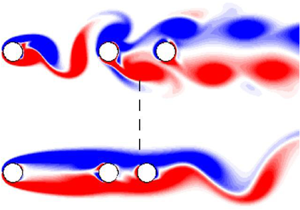
Figure 5. Instantaneous flow visualisations for three-body systems. The first two bodies are cylinders separated by  $p=5.0$ while a third body (cylinder or plate) is placed different distances
  ${p_2}$ from the second cylinder. All images are at maximum lift on the second cylinder. Dashed lines mark the end of the absolutely unstable region
  ${L_{{A}}}$ in the two-cylinder set-up.
The results are striking. For values of  ${p_2} - D/2 > {L_{{A}}}$ (we consider the most upstream point of the body as the first point to cause perturbation in the flow), the presence of the third body in either geometry has essentially no impact on the flow structure. The convectively unstable shear layers simply pass over the third body. No disturbance is felt upstream as expected for a convectively unstable flow. Further, as the flow on the wake centreline is close to stationary, the presence of the third body that forces the flow velocity to exactly zero at its surface does not introduce any significant disturbance downstream. Comparing images down each column as
  ${p_2}$ is reduced shows that the position of the first three vortex pairs in the wake is unaffected by the introduction of the third body, and comparing across rows shows the structure is also insensitive to the shape of the third body.
Moving the third body to a distance  ${p_2} - D/2< {L_{{A}}}$ from the second body (but not too close) has a profound impact on the flow as shown in the very bottom images of figure 5 where
  ${p_2} = 2.0$. This places the most upstream point of the body
  $1.5D$ from the centre of the second body, or inside the absolutely unstable region. The vortex shedding from the first cylinder is completely suppressed, and with the loss of the impinging vortices on the second cylinder the two-row structure is also destroyed. The flow transits to a new global state with a lower-frequency vortex shedding in the wake of the array as evidenced by the longer-wavelength vortex shedding apparent in the bottom images of figure 5.
The results shown in figure 5 demonstrate the cloaking and broadcasting phenomena. They show that these phenomena occur in a way that is independent of the details of the third-body geometry, but is strongly dependent on the third-body position. This strong dependence on position is consistent with the existence of absolutely and convectively unstable regions of the mean flow, and the boundary between these regions providing a threshold for the position of the third body to be broadcast (trigger a global flow change) or to be cloaked (have almost zero global impact).
To check the accuracy of the presented data and sensitivity to the location of the third cylinder, we performed simulations at smaller increments of  ${p_2}$ in the range of
  ${p_2} - D/2 \approx {L_{{A}}}$. Flow visualisations for these cases are illustrated in figure 6.

Figure 6. Instantaneous flow visualisations for three-body systems in the broadcasting, transition and cloaking states for  $p=5.0$ and
  ${p_2} =2.0$,
  $2.1$ and
  $2.2$, respectively. All images are shown at an instant of maximum lift on the second cylinder.
These images show that in a very small range of positions, where the most upstream point of the third body is around  $1.65$ from the centre of the second cylinder, the broadcasting phenomenon shifts to a cloaking phenomenon through a small transition region. We note that the appearance of this transition flow, which consists of a single row of vortices shed into the eventual wake (figure 6,
  ${p_2} =2.1$), is similar to that of the transition state of the two-cylinder system (figure 3,
  $p =4.0$) before the appearance of the two-row structure. In the three-cylinder case, there is a vortex formation behind the most upstream cylinder, a short region of the two-row structure behind the second body, followed by a single-row vortex formation with a lower frequency.
Figure 7 shows the mean drag coefficient  $\overline {C_D}$ on the third cylinder in different positions behind the second cylinder
  ${p_2}$ with consistent
  $p=5.0$. When
  ${L_{{R}}} > {p_2} -D/2> {L_{{A}}}$ the mean drag decreases to values very close to zero. The transition from a broadcasting to cloaking state is concurrent with a sudden drop in the drag. Beyond the
  ${L_{{R}}}$ region and the end of the two-row structure,
  $C_D$ increases again.

Figure 7. A plot of  $\overline {C_D}$ as a function of
  ${p_2}$ for a three-cylinder system with consistent
  $p=5.0$ and different
  ${p_2}$. Vertical solid lines mark locations of
  ${L_{{A}}}$ calculated from the local stability analysis and of
  ${L_{{R}}}$ calculated from the mean-flow streamlines.
The results presented for  $p=5.0$ can be generalised to a range of
  $p$. Figure 8 plots both
  ${L_{{A}}}$ and
  ${L_{{R}}}$ as a function of the pitch
  $p$, where both lengths are relative to the centre of the second cylinder, for the range where the two-row structure is observed (
 $p \geqslant 4.6$) from the two-cylinder system. This plot therefore provides a prediction of the range of the broadcasting and cloaking regions from the local stability analysis – the broadcasting region can occupy the wake of the second cylinder up to
  ${L_{{A}}}$, and the cloaking region occupies the wake for the second cylinder from
  ${L_{{A}}}$ up to at least
  ${L_{{R}}}$.

Figure 8. Mean recirculation length  ${L_{{R}}}$ (
 $\bullet$) and the length of the locally absolutely unstable region
  ${L_{{A}}}$ (
 $\triangle$) for two-cylinder system as a function of
  $p$ using the local stability analysis. The
  ${L_{{A}}}$ data evaluated by simulation are presented with
  $\times$ and
  $+$ for upper and lower boundaries, respectively. The dashed lines connecting these data are cubics of best fit in the form of
  $L_{A_{max}} = -0.694p^3 + 11.071p^2 - 58.829p+ 105.826$ and
  $L_{A_{min}} = 2.083p^3 - 36.25p^2 + 210.666p - 407.45$.
Also shown in figure 8 are the values of the threshold between the broadcasting and cloaking regions found simply by running simulations with a third body placed at a varying distance downstream. The body position plotted is the distance from the centre of the second cylinder to the most upstream point of the third cylinder as it is theorised that this is the first point to perturb the absolutely unstable region. The method for finding this threshold is illustrated for the example case at  $p=5.0$ above in figures 5 and 6. These direct measurements using three bodies follow closely the values from the local stability analysis using two bodies for
  $p \leqslant 5.8$. For
  $p > 5.8$ the distance between the first two cylinders is so large that any feedback mechanism between the absolutely unstable region and the upstream cylinder is broken, and the presence of the third body in
  ${L_{{A}}}$ ceases to cause a global change of the flow. The two-row structure persists, with the closely spaced second and third cylinders essentially behaving as a single elongated body.
We note here that the local stability analysis is simplified and the quantitative match between the position of the absolute–convective boundary and the location of the third body which triggers the broadcasting phenomenon may be coincidental. We also note that the phenomenon of a lower bound on the third body position is not predicted at all, and discussion of this point is provided in § 3.4.
3.4. Establishment of a lower bound for the body position that can trigger the global change
A phenomenon that is not predicted by the local stability analysis is the appearance of a lower boundary on the downstream distance of the third body to trigger the global change in state and broadcasting. However, the direct measurements show this very clearly. Figure 9 shows a series of instantaneous flow visualisations for increasing  ${p_2}$ for a constant
  $p=5.2$. For very short
  ${p_2}$ (the first value shown is
  ${p_2} = 1.2$, which gives a gap between the second and third cylinders of
  $0.2D$) there is clear vortex shedding in the first gap, and the wake of the array is clearly in the two-row convective structure. However, slightly increasing to
  ${p_2} = 1.3$ sees the vortex shedding in the first gap cease as the global change in state is triggered and the wake transits to a modified Kármán wake with reduced frequency. There is therefore a lower boundary for the appearance of the global instability around
  ${p_2} = 1.3$ for
  $p = 5.2$. This global state remains until
  ${p_2} = 2.2$, when the most upstream point of the third cylinder leaves the predicted absolutely unstable region and the flow moves back to the convectively unstable wake structure, in line with the prediction from the two-cylinder system.

Figure 9. Instantaneous flow visualisation of the flow before, across and after the broadcasting region for  $p=5.2$ and varying
  ${p_2}=1.2$, 1.3, 1.7, 2.1,
  $2.2$ and
  $2.3$. All the visualisations are presented at the instant of the maximum lift on the second body.
The lower boundary is a reasonably ‘hard’ transition, with the vortex shedding in the first gap remaining periodic when the third cylinder position is below the lower boundary, and an almost steady flow occurs once the third cylinder moves beyond the lower boundary. The time histories of  $C_L$ and
  $C_D$ for
  $p=5.2$ and
  $p_2=1.2$,
  $1.3$,
  $1.4$ and
  $1.5$ are presented in figure 10. When
  $p_2=1.2$ – below the lower boundary –
  $C_L$ and
  $C_D$ are periodic. However, increasing to
  $p_2=1.3$ sees a marked drop in the magnitude of fluctuation of the lift and drag coefficients. There is some modulation in the amplitude of
  $C_L$ and a variation in
  $C_D$ that occurs over a very long period which rapidly reduces further in magnitude as
  $p_2$ is increased further beyond the lower boundary.

Figure 10. The time histories of (a,c,e,g)  $C_D$ and (b,d,f,h)
  $C_L$ on the first cylinder for three-cylinder system with
  $p_1=5.2$ and (a,b)
  $p_2=1.2$, (c,d)
  $p_2=1.3$, (e,f)
  $p_2=1.4$ and (g,h)
  $p_2=1.5$. Note the drop in the mean drag and lift fluctuation between
  $p_2 = 1.2$ and
  $p_2 = 1.3$ as the lower bound is crossed – the range on the plots has been adjusted to show any variation beyond the lower bound.
The lower boundary is an increasing function of  $p$. Figure 11 shows a series of flow images for
  $p = 5.8$. Here, with
  ${p_2} = 1.9$, the flow is in the convectively unstable structure; a slight increase to
  ${p_2} = 2.0$ sees the appearance of the new global state which suppresses the vortex shedding in the first gap; and a further slight increase to
  ${p_2} = 2.1$ sees the reappearance of the convectively unstable structure.

Figure 11. Instantaneous flow visualisation of the flow before, across and after the broadcasting region for  $p=5.8$ and varying
  ${p_2}=1.9$,
  $2.0$ and
  $2.1$. All the visualisations are presented at the instant of the maximum lift on the second body.
This lower boundary is presented for  $p \geqslant 5.2$ in figure 8. Despite the almost constant upper boundary, the lower bound markedly increases such that broadcasting happens only for a very short range of
  ${p_2}$ when
  $p=5.8$, and the feedback mechanism, and therefore the broadcasting, disappears for
  $p\geqslant 6.0$. A perturbation in the region between the lower and upper bounds leads to the broadcasting phenomenon.
3.5. Characterisation of the new global state
The transition to a new global state and the broadcasting phenomenon causes the flow to settle to a structure with no vortex shedding in either the first or second gap, and a low-frequency Kármán wake behind the third cylinder. This change in structure is also clearly detected in the scalar measurements of the flow. Contour plots of mean drag coefficient  $\overline {C_D}$, maximum lift coefficient
  $C_{L_{max}}$ and primary frequency
  $f$ with varying
  $p$ and
  ${p_2}$ for each cylinder are presented in figures 12, 13 and 14, respectively. The acquired lines for the upper and lower boundaries of the broadcasting region from figure 8 are also plotted on the contours. These boundaries clearly coincide with the sudden change in value of the contours of all the cylinders which is evidence of a change in structure of the flow and the forces.

Figure 12. The contours of mean drag coefficient  $\overline {C_D}$ as a function of
  $p$ and
  ${p_2}$ for the first cylinder (left), second cylinder (centre) and third cylinder (right). All the contours are produced using a common colour map. The dashed lines are the upper and lower boundaries obtained from figure 8.

Figure 13. The contours of maximum lift coefficient  $C_{L_{{max}}}$ as a function of
  $p$ and
  ${p_2}$ for the first cylinder (left), second cylinder (centre) and third cylinder (right). All the contours are produced using a common colour map. The dashed lines are the upper and lower boundaries obtained from figure 8.

Figure 14. The contours of primary frequency  $f$ as a function of
  $p$ and
  ${p_2}$ for the first cylinder (left), second cylinder (centre) and third cylinder (right). All the contours are produced using a common colour map. The dashed lines are the upper and lower boundaries obtained from figure 8.
Figure 12 shows that out of the broadcasting region,  $\overline {C_D}$ decreases from the first to the third cylinder. However, in the broadcasting region there is a decrease in the value of
  $\overline {C_D}$ from the first to the second cylinder (in fact, at times the mean drag on the second cylinder is negative, resulting in a slight thrust) while it increases again on the third cylinder. Inside the broadcasting region the first and second cylinder have a lower value of
  $\overline {C_D}$ than the third cylinder.
In contrast, all the cylinders experience a decrease in  $C_{L_{max}}$ in the broadcasting region as shown in figure 13; however, this decrease is less significant for the third cylinder. This is as expected for the observed flow structure – the lack of any vortex shedding in the cylinder gaps means the fluctuating lift should be small on the upstream cylinders, and the reduced wake width of the modified Kármán wake should also coincide with a reduced lift force. Outside of the broadcasting region when the flow settles to the two-row convective structure, the second cylinder has the higher
  $C_{L_{max}}$ in comparison to the first and third cylinders. Again, this fits with the flow structure – the second cylinder is exposed to impinging vortices being shed from the first cylinder, and the fluctuating wake.
The frequency contours in figure 14 show that all the cylinders have essentially similar values of primary frequency either in the cloaking or broadcasting regions. In the cloaking region, the frequency is set by the vortex shedding in the first gap, and vortices at this frequency are simply convected past the second and third cylinders. In the broadcasting region, a new global state is triggered and all the three cylinders behave as almost a single more streamlined body and therefore share a common frequency. This common frequency is less than the frequency of vortex shedding from a single cylinder or in the cloaking region.
4. Sensitivity analysis of two-cylinder system
The sensitivity analysis outlined in § 2.3 is conducted on the mean flow of the two-cylinder system with different values of  $p=4.8$,
  $5.2$,
  $5.6$ and
  $6.0$ in an effort to explain the presence of the lower limit for the third cylinder position to control the global mode. The mean flows for these values of
  $p$, and the sensitivity fields for the leading global mode on these mean fields, are presented in figure 15. These values are chosen as they span three scenarios:
(i) For
 $p = 4.8$, there is only an upper limit. Placing the third cylinder closer than this always suppresses vortex shedding in the first gap.
(ii) For
$p = 5.2$ and $5.6$, there is an upper and lower limit. Placing the third cylinder between these limits suppresses vortex shedding, but placing the third cylinder closer than the lower limit sees vortex shedding reinstated.(iii) For
$p = 6.0$, there are no limits, and a third cylinder can be placed anywhere without any impact on the vortex shedding in the first gap.


Figure 15. Left: vorticity contours of the mean flow where red/blue contours mark positive/negative vorticity overlaid with separating streamlines. Right: contours of the sensitivity field for the leading global mode on this mean, where dark/light colours mark low/high values. Four cases for the two-cylinder system are shown with (a)  $p=4.8$, (b)
  $p=5.2$, (c)
  $p=5.6$ and (d)
  $p=6.0$. The dashed circles represent the location where the most upstream point of the circle coincides with the location of the lower boundary and the solid circles have their most upstream point coinciding with the location of the upper boundary as shown in figure 8.
The first point to note from figure 15 is that the sensitivity field in the gap looks almost similar in all the cases – the change in the position of the second cylinder has little impact on the flow structure and therefore little impact on the mean and global mode. However, the structure of the sensitivity field behind the second cylinder varies for different  $p$.
$p$.
Two main features are identified with increasing  $p$. First, the location of the most sensitive region is initially located in two bands symmetric about the wake centreline that slant from the most transverse points of the cylinder towards a point on the centreline around
  $2D$ downstream. These bands seem to track the location of the separating streamline. For
  $p = 4.8$, the most sensitive location is located around
  $1D$ downstream of the centre of the second cylinder, and around
  $0.6D$ transverse from the wake centreline. Increasing
  $p$ sees the most sensitive region move upstream and towards the centreline, so that at
  $p=5.6$ the most sensitive region is almost at the cylinder surface directly transverse of the cylinder centre. Increasing further to
  $p=6.0$ sees the most sensitive region move from these separating-streamline bands into the core of the mean recirculation region.
The second feature is the development of a secondary sensitive region in the mean shear layers that grows in relative intensity with increasing  $p$. However, these regions never contain the most sensitive points in the flow.
This shift in the location of the most sensitive region perhaps explains why no cylinder position can suppress or control the global mode when  $p\geqslant 6$; once the sensitive regions move inside the mean recirculation region, any perturbation that triggers them has no mechanism to propagate to other regions of the flow as it is trapped inside the separating streamline. However, for lower
  $p$ where the sensitive regions are on or just outside the separating streamline, perturbations introduced on this streamline can be transported to the sensitive region, amplified and transported back, forming a feedback loop that can lead to large growth and provide a physical mechanism to control the global mode and therefore broadcast the location of the third cylinder. This is consistent with the observed behaviour – the upper boundary of the third cylinder position that controls the global mode is almost constant at around
  $p_2 \simeq 2$, and the images in figure 15 show this coincides with a position where the most upstream point of the third cylinder comes into contact with a region of increased sensitivity aligned with the mean separating streamline. The sensitivity analysis supports the phenomenological argument for an upper limit on the third cylinder position from the local stability analysis presented in § 2.2.
What is still not present is a clear indication of why the intermediate values of  $p=5.2$ and
  $p=5.6$ present a lower limit for the location of a third cylinder that can suppress the global mode leading to the vortex shedding in the gap. There is some indication of the sensitivity field displaying a local maximum on the wake centreline which could coincide with the sensitivity (and therefore control) first rising, then falling again as the third cylinder is moved closer to the second. However, this local maximum is present in all the sensitivity fields whether or not a lower limit is identified, and so this condition does not seem sufficient to explain the presence of the lower limit.
A more nuanced explanation may be that the current analysis is linear, and performed on the mean flow which itself is a function of the complete nonlinear flow. The third cylinder is certainly not a small perturbation, and will therefore induce nonlinear effects and therefore a mean-flow correction. So, simply placing the third cylinder in regions where the two-cylinder mean flow is sensitive may not control the global mode, but instead remove the regions of sensitivity by modifying the mean flow in a way that these sensitive regions disappear.
We note here that another avenue of analysis may be via the sensitivity framework of Marquet, Sipp & Jacquin (Reference Marquet, Sipp and Jacquin2008), which more directly assesses the impact of the introduction of a steady body force, such as that introduced by the drag on the third cylinder. However, the application of that framework to the current problem is not obvious, as here we assess the mean flow, not a steady flow. The definition of the perturbing body force in the mean is not straightforward, and we leave this analysis to future work.
To further investigate this, the mean flow and sensitivity field for the three-cylinder system with  $p_1=5.2$ and two critical locations for
  $p_2=1.2$ and
  $1.3$, before and after the lower boundary defined on figure 8, are studied and presented in figure 16.

Figure 16. The mean flow (top) and sensitivity field (bottom) for three-cylinder system with  $p_1=5.2$ and (a)
  $p_2=1.2$ and (b)
  $p_2=1.3$.
As shown in figure 9, this minor change in location of the third cylinder has a marked impact on the flow with periodic vortex shedding occurring in the first gap when  $p_2 = 1.2$, and an almost steady flow in this first gap when
  $p_2 = 1.3$. This global change is also reflected in the mean-flow structure, and the subsequent sensitivity field which grows on this mean.
The mean-flow structure in the first gap for  $p_2 = 1.2$ when vortex shedding occurs is very similar to that of the two-cylinder problem presented in figure 15(b), and accordingly the sensitivity field in this first gap is also similar. However, the presence of the third cylinder modifies the mean field such that the sensitive regions of the flow behind the second cylinder – which for the two-cylinder flow tracked the separating streamline down to the wake centreline – track the separating streamlines which enclose a region between the second and third cylinders. The effective streamlining of the two rearmost bodies acting as an elongated body breaks the feedback.
For the case where  $p_2 = 1.3$, the most sensitive region is clearly behind the third body; however, there is also a highly sensitive region that forms between the second and third bodies and extends upstream along the separating streamlines. This is a consequence of the strong modification of the mean flow via the suppression of the vortex shedding in the first gap.
The observations presented in figure 16 provide some indication that the impact of the third cylinder is not just to introduce a disturbance in areas which are sensitive, but potentially to modify the mean flow such that these sensitive regions disappear. This occurs when the third cylinder is very close to the second, forming an effective longer streamlined second body. Of course this conclusion comes with the caveat that the analysis performed is linear and the impact of the presence of the third cylinder has already modified the mean flow via a nonlinear correction.
5. Linear stability of the mean flows of the two- and three-cylinder systems
The discussion of the sensitivity results presented in § 4 suggests that a linear analysis of the mean is not sufficient to completely explain the transition between the cloaking and broadcasting states. However, once each state is saturated, a linear analysis of the mean does recover the essential dynamics of the flow as explained below.
The forward modes for the two-cylinder system with  $p=5.2$, three-cylinder system with
  $p=5.2$ and second gap distances
  $p_2=1.2$ and
  $p_2=1.3$ are presented in figure 17. The frequency
  $f$ from simulations and the forward (or global) mode are presented for each case.

Figure 17. The vorticity of the real component of the global mode, frequency measured from the simulations and the frequency of the leading forward (global) mode for (a) the two-cylinder system with  $p=5.2$, (b) the three-cylinder system with
  $p=5.2$ and
  $p_2=1.2$ and (c) the three-cylinder system with
  $p=5.2$ and
  $p_2=1.3$.
The first two images compare the two- and three-cylinder cases where there is vortex shedding in the first gap (the third cylinder is cloaked). In both cases, the mode structure in the first gap is similar, reflecting the fact that the vortex shedding structure is similar. Because this vortex shedding sets the global frequency, the measured frequency in both cases is almost the same, and in both cases the frequency of the global mode closely matches the measured frequency.
The third image shows a three-cylinder case where there is no vortex shedding in the first gap (the third cylinder is broadcast). There is a distinct change in the structure of the mode in the gap, with an area of almost no growth directly behind the first cylinder, with the growth focused in the centre of the wake of the third cylinder. The measured frequency is lower than in the two-cylinder and cloaked cases, and again the frequency of the global mode closely matches the measured frequency.
These results suggest that once the mean is saturated, the flow in all cases is well described in terms of the mean and a single mode, even if the saturation process for the transition between the two modes is not explained by a linear model.
6. Conclusions
This study shows that a tandem two-cylinder system generates a two-row shear layer structure once the pitch is long enough to allow vortices to form and to impinge on the second cylinder.
These shear layers simply convect the forcing imposed by the vortex shedding from the first cylinder, maintaining its frequency and spatiotemporal symmetry. This flow structure persists in larger arrays of tandem bodies – bodies of varying size, shape and separation distance can be included in the wake at a moderate distance downstream with little impact on the general flow. The presence of the third body is effectively cloaked.
However, placing a third body close to the rear of the second cylinder can have a notable effect, completely suppressing the vortex shedding from the first cylinder and destroying the two-row structure, globally broadcasting the presence of the third body. Most notably, this behaviour is very sensitive to the position of the third body, with both an upper and a lower limit on the downstream distance of the third body which will trigger this broadcasting behaviour. The global change in the flow state is clearly identified in the forces on all three bodies.
A phenomenological explanation for the presence of the upper limit in this position is provided from a local stability analysis of the mean flow which identifies the two-row structure as convectively unstable, except for a small region directly adjacent to the rear of the second cylinder which is weakly absolutely unstable. Placing a third body in this absolutely unstable region (at distances less than around  $1.5D$ from the centre of the second cylinder) has the potential to trigger a global instability and therefore the change to a new global state. This finding is supported by a global sensitivity analysis. However, the existence of a lower limit (i.e. bodies placed very close to the second cylinder do not trigger a change) indicates that the disturbance of this absolutely unstable region is not sufficient to explain the broadcasting phenomenon which appears to be nonlinear.
Acknowledgements
N.H. acknowledges the support of Swinburne University of Technology via a Swinburne University Postgraduate Research Award (SUPRA). J.S.L. acknowledges the financial support of the Australian Research Council (ARC) via Discovery Project DP150103177, and the support of the National Computational Infrastructure, which is supported by the Australian government.
Declaration of interests
The authors report no conflict of interest.


