2.1. Wind tunnel and flow cases

Experiments were performed in the TFT boundary-layer wind tunnel already described in detail in Mohammed-Taifour et al. (Reference Mohammed-Taifour, Schwaab, Pioton and Weiss2015) and Mohammed-Taifour & Weiss (Reference Mohammed-Taifour and Weiss2016). Briefly, the low-speed wind tunnel is of blow-down type, with a test section 3 m in length and 0.6 m in width, as illustrated in figure 1. In the first half of the test section, a ZPG boundary layer develops on the upper surface and separates because of the APG imposed by the diverging test-section floor. The boundary layer subsequently reattaches due to the FPG that occurs when the floor converges again. The use of a bleed slot ensures that the boundary layer on the lower surface stays attached on the contoured part of the test-section floor. This slot connects directly to the atmosphere, while the interior of the test section is maintained at a slightly elevated pressure by a mesh positioned at the exit.

Figure 1. (a) Average wall-pressure coefficient $c_p$ measured on the test-section centreline ($z=0$ m) along the streamwise axis. (b) Profile sketch of the test section. The black solid line corresponds to the Large TSB of Mohammed-Taifour & Weiss (Reference Mohammed-Taifour and Weiss2016), the red dashed line is the new Medium TSB and the blue dash-dotted line is the new Small TSB.

As shown in figure 1, the diverging test-section floor generates a strong adverse pressure gradient starting at about $x \simeq 1.4$ m, where $x=0$ marks the entrance of the test section. The original geometry of the test-section floor creates the pressure distribution depicted with black squares, as already investigated by Mohammed-Taifour & Weiss (Reference Mohammed-Taifour and Weiss2016). In the present work, a set of two foam blocks are inserted in the aft part of the contoured test-section floor so that the APG stays the same but two new zones of FPG are created more upstream of the original geometry, thereby generating two new separation bubbles of smaller sizes. The contour depicted with the blue dashed line in the lower part of figure 1 creates a $c_p$ distribution for the ‘Small TSB’, while the one with the red dash-dot line creates a pressure distribution for the ‘Medium TSB’. The original $c_p$ distribution of Mohammed-Taifour & Weiss (Reference Mohammed-Taifour and Weiss2016) results in a ‘Large TSB’. Note that $c_p(x) = 2(p(x)-{p_{ref}})/\rho U_{ref}^2$, where ${p_{ref}}$ and ${U_{ref}}$ refer to the static pressure and velocity at the entrance of the test section, respectively (details regarding the instrumentation used in the wind tunnel are given in § 2.2). For all experiments, the reference velocity is ${U_{ref}}=25\ \textrm {m}\ \textrm {s}^{-1}$ and the atmospheric air density is $\rho \simeq 1.2\ \textrm {kg}\ \textrm {m}^{-3}$. Also, at $x_{in}=1.1$ m the incoming boundary-layer thickness is $(\delta _{99})_{in}=28$ mm and the momentum thickness is $\theta _{in}=3.0$ mm, which implies a Reynolds number $Re_{\theta _{in}} \simeq 5000$, as in Mohammed-Taifour & Weiss (Reference Mohammed-Taifour and Weiss2016).

The pressure distributions generated experimentally in the TFT Boundary-Layer Wind Tunnel are compared to those obtained by other researchers in figure 2, with relevant data also listed in table 1. The available database consists of the experimental results of Perry & Fairlie (Reference Perry and Fairlie1975) and Patrick (Reference Patrick1987), as well as the CFD results of Na & Moin (Reference Na and Moin1998a), Abe (Reference Abe2017), Coleman et al. (Reference Coleman, Rumsey and Spalart2018) (noted CRS) and Wu & Piomelli (Reference Wu and Piomelli2018). In order to provide a meaningful comparison, a common datum is required to position the different pressure distributions. Following Coleman et al.'s (Reference Coleman, Rumsey and Spalart2018) suggestion, the streamwise position $x_{V_{top}=0}$ where the transpiration profile changes sign from suction to blowing was chosen as a common reference since it can easily be obtained from all published data, except for the experiment of Perry & Fairlie (Reference Perry and Fairlie1975), where the calculated transpiration profile of Cheng et al. (Reference Cheng, Pullin and Samtaney2015) was used instead. For the present data and those of Patrick (Reference Patrick1987), $x_{V_{top}=0}$ was defined by using the vertical velocity measured furthest away from the test surface as a proxy for the transpiration profile. The streamwise position was furthermore normalized by the momentum thickness $\theta _0$ that the ZPG boundary layer would reach at $x_{V_{top}=0}$ in the absence of any pressure gradient. This value was calculated from the published data by integrating the von Kármán integral equation $\textrm {d}\theta / \textrm {d}x = c_f/2$ from its value $\theta _{in}$ at a specified ZPG position in the original publication to its value $\theta _0$ at $x_{V_{top}=0}$ (for the present experiments the reference streamwise position is $x_{in}=1.1$ m). The classical ZPG power law $c_f/2 = 0.0128Re_{\theta }^{-0.25}$, from Schlichting (Reference Schlichting1968, p. 600), was used in the integration. The Reynolds numbers $Re_{\theta _{in}}$ at each reference position and the corresponding $Re_{\theta _0}$ at each $x_{V_{top}=0}$ are listed in table 1, where it can be seen that, depending on the choice of reference position in the original article, $Re_{\theta _0}$ can be as much as twice $Re_{\theta _{in}}$.

Figure 2. Streamwise distributions of wall-pressure coefficient.

Table 1. Definition of the main pressure-induced TSB features: data with ($^*$) are from the present study; CRS stands for Coleman et al. (Reference Coleman, Rumsey and Spalart2018); $\theta _{in}$ and $\theta _0$ are the momentum thicknesses at the reference position and $x_{V_{top}=0}$, respectively; $V_{top}$ is the transpiration profile imposed in numerical simulations and $H_{V_{top}}$ its height above the wall; $L_b$ is the distance between transitory detachment (TD) and transitory reattachment (TR); $L_p$ is the distance between the maximum APG and FPG; $H_b$ is the maximum distance between the mean dividing streamline and the wall; $w$ is the width of the test section for experimental data and the spanwise extent of numerical domains; finally, [APG] and [FPG] are defined as $\theta _0\cdot [{\textrm {d}C_p}/{\textrm {d}x}]_{max}\times 10^{-3}$ and $\theta _0\cdot [{\textrm {d}C_p}/{\textrm {d}x}]_{min}\times 10^{-3}$, respectively.

Several noteworthy features can be observed in figure 2. First, most of the $c_p$ distributions show the classical bell-shaped form expected from a suction-and-blowing transpiration profile. Notable exceptions are those obtained in the present work, which do not go back down to $c_p=0$ after reattachment. This is due to the geometry of the wind-tunnel test section, which has the same height upstream and downstream of the pressure-gradient zone. Bringing $c_p$ down to zero would require a smaller height in the aft part to compensate for the mass flow removed by the bleed slot (approximately 10 % of the incoming mass flow, corresponding to $c_p \simeq 0.2$). The same can be said from the pressure distribution of Patrick (Reference Patrick1987), who used a similar experimental set-up. The third exception is the pressure distribution from Perry & Fairlie (Reference Perry and Fairlie1975), which features a mild APG starting much earlier than the others, and a very strong FPG to close the bubble.

The Patrick (Reference Patrick1987) pressure distribution also stands out because of its clear apex in the downstream half of the bell-shaped curve, which is interpreted in his original report as the result of the impingement and partial stagnation of the reattaching flow. A similar feature, albeit at a more modest scale, can be seen in most other cases. Table 1 lists the wall-normal aspect ratios of the separation bubbles, defined as the height $H_b$ of the recirculation zone divided by its length $L_b$, where $H_b$ is the maximum distance between the wall and the mean dividing streamline, whereas $L_b$ is the distance between transitory detachment and reattachment. Comparing this parameter with the $c_p$ curves of figure 2 reveals that the peak in the pressure distribution is more pronounced for larger wall-normal aspect ratios. This is consistent with the Patrick (Reference Patrick1987) explanation of impingement being responsible for the pressure peak, though the large Reynolds number in his case might also play a significant role.

Generally speaking, except for Perry & Fairlie (Reference Perry and Fairlie1975), most $c_p$ distributions appear to cluster between the Coleman et al. (Reference Coleman, Rumsey and Spalart2018) cases A and C. The pressure distributions from Na & Moin (Reference Na and Moin1998a), Abe (Reference Abe2017) (case LB) and Wu & Piomelli (Reference Wu and Piomelli2018) are very close, mostly because the latter authors designed their simulations to reproduce Na and Moin's results. The Coleman et al. (Reference Coleman, Rumsey and Spalart2018) case A has comparable pressure gradients but imposed on a shorter distance. In contrast, their case C imposes smaller gradients but over a larger distance. The Patrick (Reference Patrick1987) distribution appears shorter, although it can be seen as an artefact caused by the larger Reynolds number that results in a larger $\theta _0$. Finally, the pressure distributions generated in the TFT Boundary-Layer Wind Tunnel appear to have APGs reasonably close to Na & Moin (Reference Na and Moin1998a) and others, whereas our FPGs are closer to the Coleman et al. (Reference Coleman, Rumsey and Spalart2018) case C (see also the maximum APG and FPG listed in table 1 for each case).

To provide further insight into the different flow cases, the normalized vertical velocity $V/{U_{ref}}$ measured at the edge of our experimental field of view ($y/\theta _0 \simeq 17$) is plotted in figure 3 as a function of the normalized streamwise distance. Only the velocity data from Na & Moin (Reference Na and Moin1998a), Coleman et al. (Reference Coleman, Rumsey and Spalart2018) and Patrick (Reference Patrick1987) were available for comparison at $y/\theta _0 \simeq 17$. The main interesting feature of figure 3 is that, in contrast to the present data, all available flow cases are approximately symmetrical, with the same amplitudes for suction and blowing. However, the data obtained in the TFT wind tunnel exhibit a larger amplitude in the suction part ($V>0$) than in the blowing part ($V<0$), which is consistent with the fact that the FPG is smaller than the APG (see table 1 and figure 2). Furthermore, the suction velocity in our Large TSB appears to be fairly close to that of Na & Moin (Reference Na and Moin1998a), but significantly smaller than in the Patrick (Reference Patrick1987) flow. On the other hand, the blowing velocity of our Medium TSB is very close to the Coleman et al. (Reference Coleman, Rumsey and Spalart2018) case C. This compilation of velocity data is fully consistent with the pressure distributions of figure 2.

Figure 3. Streamwise distributions of vertical velocity at $y/\theta _0 \simeq 17$. The data from Na & Moin (Reference Na and Moin1998a) were interpolated from their figure 19.

Based on a comparison of the normalized separation lengths $L_b/\theta _0$ and aspect ratios $H_b/L_b$ listed in table 1, and based on the pressure and velocity data from figures 2 and 3, we conclude that our Large TSB is probably geometrically closest to the Na & Moin (Reference Na and Moin1998a) flow, despite a significant difference in Reynolds number. Similarly, our Medium TSB is probably the closest to the Coleman et al. (Reference Coleman, Rumsey and Spalart2018) case C, with a factor of approximately 2 in Reynolds number and a notable difference in pressure distribution. Of course, two TSB flows would only be identical if the Reynolds numbers and pressure distributions were identical, or equivalently if the Reynolds numbers were identical and the same transpiration profiles were imposed at the same wall-normal distance.

2.2. Instrumentation

The experimental techniques used in the present work were essentially the same as in Weiss et al. (Reference Weiss, Mohammed-Taifour and Schwaab2015) and Mohammed-Taifour & Weiss (Reference Mohammed-Taifour and Weiss2016) and will only be described briefly. The average wall pressure was measured using two Scanivalve DSA3217 pressure scanners and the wall-pressure fluctuations with several Meggitt 8507C-1 piezoresistive pressure transducers. The estimated uncertainty of the measured values is ${\pm } 0.7\,\%$ and ${\pm } 5\,\%$ for the mean and fluctuating pressure, respectively (Weiss et al. Reference Weiss, Mohammed-Taifour and Schwaab2015). Necessary corrections of the fluctuating pressure data to remove the low-frequency facility noise caused by small mass-flow fluctuations from the flow mover were made by applying the noise-correction method of Weiss et al. (Reference Weiss, Mohammed-Taifour and Schwaab2015), which consists in removing the part of the signal that is coherent with the noise measured near the entrance of the test section. The forward-flow fraction $\gamma$, defined as the percentage of time that the near-wall flow goes in the main, positive streamwise direction, was measured with the MEMS calorimetric shear-stress sensor introduced by Weiss et al. (Reference Weiss, Schwaab, Boucetta, Giani, Guigue, Combette and Charlot2017). The uncertainty in $\gamma$ was estimated at ${\pm }2\,\%$ based on a comparison with the classical thermal-tuft probe of Schwaab & Weiss (Reference Schwaab and Weiss2015). All single-point unsteady signals were digitized with a 24-bit National Instruments NI-PXIe-4492 data acquisition card at a sampling rate of 2 kHz and low-pass filtered with the embedded anti-aliasing filter. Power spectral densities were computed using Welch's modified periodogram algorithm with 50 % overlap and a Hamming window (Bendat & Piersol Reference Bendat and Piersol2010).

The wall-pressure fluctuations were obtained by connecting the piezoresistive pressure transducers to pressure taps installed on the test surface with 15 mm long flexible tubing. This set-up resulted in an organ-pipe resonance frequency of approximately 2 kHz for the tube-and-pressure-tap system. Using the boundary-layer displacement thickness $\delta ^*=3.80$ mm measured at $x_{in}=1.1$ m (ZPG) and the Nyquist frequency $f=1$ kHz of the pressure signals, the maximum normalized frequency that can be resolved is $\omega \delta ^*/{U_{ref}} = 0.95$, with $\omega =2{\rm \pi} f$. This value is lower than for dedicated acoustic measurements using pinholes (Simpson et al. Reference Simpson, Ghodbane and McGrath1987; Bull Reference Bull1996). Thus, our pressure data are mainly concentrated within the energetic low- and medium-frequency range observed under the turbulent separation bubbles and does not resolve the high-frequency fluctuations present under the attached incoming boundary layer (see also the discussion pertaining to figures 10 and 15).

Planar flow velocity measurements were achieved using a high-speed, planar, two-component (2D-2C), PIV system that consists of a Litron LDY304 Nd:YLF laser, light-sheet optics and two Phantom V9.1 CMOS cameras mounted side by side. Both cameras were equipped with a 50 mm, f#2 Micro Nikkor lens to obtain a total field of view of approximately 0.20 m in the streamwise direction and 0.075 m in the wall-normal direction. The pair of cameras was moved in the streamwise direction to cover the complete length of all the separation bubbles (see figure 1). Respectively three, four and six stations were required for the Small, Medium and Large TSBs. In the case of the Large TSB, a total of five separate sequences of 3580 images were recorded at a sampling frequency of 900 Hz, thus resulting in a total dataset spanning 20 s (Mohammed-Taifour & Weiss Reference Mohammed-Taifour and Weiss2016). For the Small and Medium TSBs, in order to optimize the data storage requirements, three separate sequences of 3580 images were recorded at a reduced sampling frequency of 400 Hz for a total measuring time of 27 s. It was verified that the change of sampling frequency from 900 Hz to 400 Hz had no detrimental impact in capturing the flow statistics. The images were processed by the LaVision DaVis software (version 8.2) using a multi-pass correlation technique with 75 % overlap. The vector spacing in the object plane is 0.55 mm, which corresponds to approximately 2 % of the boundary-layer thickness at $x_{in}=1.1$ m ($\delta _{99}=28$ mm) and 13 % of $\theta _0$ ($\theta _0 \simeq 4.1$ mm).

In Mohammed-Taifour & Weiss (Reference Mohammed-Taifour and Weiss2016) the PIV data were validated by a favourable comparison with hot-wire results, both in the incoming ZPG boundary layer and in the large separation bubble. Rather than reproducing similar results, we show in figure 4 a comparison between the turbulence statistics $\bar {U}/{U_{ref}}$, $\overline {u'u'}/U_{ref}^2$, $\overline {v'v'}/U_{ref}^2$ and $-\overline {u'v'}/U_{ref}^2$ measured in our Medium TSB with the DNS results of the Coleman et al. (Reference Coleman, Rumsey and Spalart2018) case C. For both databases the $x$ axis was normalized by the distance $L_p$ between the maximum APG and the maximum FPG (also listed in table 1). Clearly, the results are rather close to one another, which is expected given the similarities in the bubble dimensions from table 1. While this favourable comparison gives confidence in the PIV data, it also shows the reduced spatial resolution and convergence of the PIV results compared to the DNS, which is a consequence of the limited resolution of the CMOS cameras, the required stitching between different fields of view and the limited integration time resulting from the finite camera memory. In order to estimate realistic uncertainty bounds for the PIV data, a detailed convergence study was performed on all measured turbulence statistics on a large number of grid points spanning the complete field of view. Specifically, the difference between the maximum and minimum value of the convergence curves over the last 30 % of the total measurement time was used as an estimate of the random uncertainty. Furthermore, the small step occurring at the boundary between two adjacent fields was quantified and used as an estimate of the systematic uncertainty. The total uncertainties estimated by this procedure are ${\pm }0.2\ \textrm {m}\ \textrm {s}^{-1}$ for the mean streamwise velocity, ${\pm }0.3\ \textrm {m}\ \textrm {s}^{-1}$ for the mean wall-normal velocity, ${\pm } 0.2\ \textrm {m}^2\ \textrm {s}^{-2}$ for the streamwise stresses, ${\pm }0.1\ \textrm {m}^2\ \textrm {s}^{-2}$ for the wall-normal stresses and ${\pm } 0.1\ \textrm {m}^{2}\ \textrm {s}^{-2}$ for the shear stresses. This translates into relative uncertainties of approximately 1 % for the mean velocities (based on the inlet velocity $U_{ref} = 25\ \textrm {m}\ \textrm {s}^{-1}$), and 4 %, 5 % and 10 % for the streamwise, wall-normal and shear stresses, respectively (based on the median stresses for the Medium TSB). These uncertainty estimates are typical of current high-speed PIV systems, e.g. Ma, Gibeau & Ghaemi (Reference Ma, Gibeau and Ghaemi2020). Nevertheless, the proximity of the test surface or unavoidable reflections from the test-section walls may locally generate larger errors.

Figure 4. Medium TSB (left) compared with the Coleman et al. (Reference Coleman, Rumsey and Spalart2018) case C (right). Black squares hide invalid PIV data in some near-wall regions.

3.1. General flow topology

Oil-film visualizations on the test surface for the three separation bubbles are shown in figure 5. The oil film was a mixture of titanium dioxide, paraffin oil and some oleic acid that was applied on the surface before turning on the wind tunnel. The images show the complete span of the test section (0.6 m) and a streamwise distance of 1 m that approximately corresponds to the region of imposed pressure variations for the Large TSB (compare with the axis system defined in figure 1). The non-dimensional spanwise axis $z^*=z/z_0$, with $z_0=0.30$ m corresponding to the half-span of the test section, is also introduced. Iso-$\gamma$ lines of constant forward-flow fraction are superimposed on the images. These lines were obtained by interpolating the values of the forward-flow fraction $\gamma$ measured with the calorimetric shear-stress sensor on a raster of $10\ \textrm {cm}\times 10\ \textrm {cm}$ on the test surface.

Figure 5. Oil flow visualizations of the three separation bubbles. (a) Large TSB. (b) Medium TSB. (c) Small TSB. Black lines: forward-flow fraction $\gamma$.

The general topology of the surface streamlines appears to be reasonably similar for all separation bubbles. In all cases, the flow is symmetric with regard to the centreline. The limiting streamlines are essentially straight in a narrow slice which spans a third of the test-section width for the Medium and Large TSBs (i.e. $\left \lvert z ^*\right \rvert <1/3$) and approximately half its width for the Small TSB ($\left \lvert z ^*\right \rvert <1/2$). Outside of this central range, strong three-dimensional effects caused by the complex flow near the corners of the test section are evident, although flow visualizations on the sidewalls did not indicate any mean separation from the sidewall boundary layers (Mohammed-Taifour & Weiss Reference Mohammed-Taifour and Weiss2016). The iso-$\gamma$ lines are consistent with the oil-film images and, although slightly curved, do not show any strong asymmetry in the near-wall flow. Surprisingly, although the ratio between mean separation length and test-section span is smaller for the Medium TSB than for the Large TSB, the size of the region affected by the corner flows is relatively similar. This indicates that, proportionally to the TSB length, the three-dimensional effects are more pronounced for the Medium TSB.

The symmetry of the shear-stress lines on the test surface necessarily precludes any significant mean out-of-plane velocity component on the test-section centreplane, as those wall streamlines are exceedingly sensitive to minute transverse pressure gradients. In that respect, the flow near the centreline can be described as quasi two-dimensional in the mean. Nevertheless, it should be emphasized that the average flow near the centreline is not necessarily the same as the flow that would be obtained if the test-section width was infinite. In a geometry-induced TSB created with a fence and splitter plate, Ciampoli & Hancock (Reference Ciampoli and Hancock2006) found that residual effects of the tunnel sidewalls are seen in the mean wall shear stress near the tunnel centreline up to a test-section width to bubble length ratio of approximately 7. This is much larger than any experiment performed so far on pressure-induced TSBs (see table 1, where $w/L_p$ is typically of the order of one). Hence, our mean TSBs are necessarily affected by the presence of the sidewalls, even near the centreline.

Because three-dimensional flow structures can only be crudely hypothesised from two-dimensional oil-film visualizations, a qualitative RANS simulation of the Medium TSB was performed using a commercial CFD software (ANSYS CFX-17.2) in order to better understand the three-dimensional nature of the average flow. The complete wind-tunnel test section was discretized with a standard hexahedral mesh composed of 20 million cells that was refined near the walls to achieve a first node value of $y^+ < 1$. The model boundaries consisted of the test-section inlet and exit, the two side walls, the ceiling and floor walls, and the boundary-layer bleed. The test-section length was extended near its entrance to match the experimental boundary-layer thickness at $x_{in} = 1.1$ m and the inlet boundary condition was set at an average velocity of $U_{ref}=25\ \textrm {m}\ \textrm {s}^{-1}$ and a turbulence level of 0.05 %, as measured experimentally (Mohammed-Taifour et al. Reference Mohammed-Taifour, Schwaab, Pioton and Weiss2015). Both the boundary-layer bleed and the test-section exit outlet conditions were set at zero gradient, and the imposed pressures were chosen by trial and error in order to reproduce as closely as possible the experimental $c_p$ distribution of figure 1. Grid convergence was deemed satisfactory based on a comparison of results obtained on three grid sizes composed of 9 (coarse), 20 (medium) and 44 (fine) million cells. Several turbulence models were tested and the BaSeLine Explicit Algebraic Reynolds Stress Model (BSL-EARSM) described in Menter, Garbaruk & Egorov (Reference Menter, Garbaruk and Egorov2012) was finally selected because it best reproduced the wall streamlines visualized experimentally (Mohammed-Taifour, Dufresne & Weiss Reference Mohammed-Taifour, Dufresne and Weiss2019).

The results of the simulation should only be interpreted qualitatively because it is well known that RANS methods are not capable of accurately reproducing many quantitative aspects of turbulent separated flows (Coleman et al. Reference Coleman, Rumsey and Spalart2018). Nevertheless, the three-dimensional structure of the simulated average flow presented in figure 6 shows several noteworthy features that help interpret the experimental wall streamlines: First, the simulated shear-stress lines on the top surface suitably reproduce the oil-film visualization of figure 5, thereby bringing credibility to the RANS results. Second, the distinction between a central zone with approximately straight shear-stress lines and two symmetrical zones with strong three-dimensional effects for $\left \lvert z \right \rvert > 0.1$ m, already apparent on the oil film, is also evident in figure 6. Finally, the RANS results clearly show that the three-dimensional nature of the wall streamlines on the top surface is not caused by separation from the sidewall boundary layers (as also verified experimentally), but rather by the signature of large-scale, longitudinal corner vortices that create a spanwise velocity component oriented towards the centreline close to the test surface. The generation of these corner vortices can be interpreted by classical secondary-flow arguments (Bradshaw Reference Bradshaw1987): the curvature of the streamlines in the potential flow imposes a lateral pressure gradient on the sidewall boundary layers (i.e. in the $y$-direction). In the upstream half of the separated region, the cross-flow profiles are directed towards positive $y$, away from the test surface. On the other hand, in the downstream half of the TSB, the cross-flow profiles are oriented towards the test surface. This translates into an upward motion of the lateral boundary layers, which flow around the corners towards the centreline of the test surface. Moving downstream, this flow pattern rolls up into two large longitudinal corner vortices. In many ways this phenomenon is reminiscent of the streamwise vortices observed in constant width wind-tunnel contractions (Mokhtari & Bradshaw Reference Mokhtari and Bradshaw1983; Bouriga et al. Reference Bouriga, Taher, Morency and Weiss2015). In the remainder of this section we will consider experimental data obtained on the test-section centreline only, where quasi-two-dimensional conditions can be observed. However, because of the three-dimensional character of the average flows discussed above, we will return to this point in § 3.4.

Figure 6. RANS simulation results showing the average flow structure in the Medium TSB. Black lines on top: wall streamlines on the left-hand side of the test surface. Coloured cuts: contours of the average spanwise velocity $\overline {W}$. Black lines on the bottom: representative streamlines showing the effects of the corner flow.

Looking back at figure 5, it can be observed that the forward-flow fraction has a constant value of $\gamma \simeq 100$ % upstream of the field of view. The threshold $\gamma =99$ %, corresponding to the position of incipient detachment (ID) according to the terminology of Simpson (Reference Simpson1989), is reached at $x \simeq 1.55$ m for all flow cases. Intermittent transitory detachment (ITD, $\gamma =80$ %) occurs at $x \simeq 1.65$ m for the Medium and Large TSBs, but not for the Small TSB, where the minimum value of $\gamma$ on the centreline lies just over this threshold (81 %, see also figure 7). For the Medium and Large TSBs, the value $\gamma =50$ % that corresponds to the average detachment line (or transitory detachment, TD) is reached at $x \simeq 1.75$ m on the test-section centreline. This threshold in not reached in the case of the Small TSB. Thus, the Small TSB does not feature any region of mean back flow in a large portion of the test section and the flow can be considered to be attached in the mean. Moving downstream, the point of mean reattachment ($\gamma =50$ %) is reached at $x = 1.90$ m for the Medium TSB and $x = 2.15$ m for the Large TSB. Finally, the positions where $\gamma =99$ % in the reattachment region, which can be dubbed ‘complete reattachment’ (CR), are reached further downstream ($x = 1.87$, $x = 2.07$, and $x = 2.27$ m for the Small, Medium and Large TSBs on the test-section centreline, respectively). Based on these measurements, the average separation length $L_b$, defined as the distance between mean detachment and mean reattachment on the test-section centreline is $L_b=0.11$ m for the Medium TSB and $L_b=0.40$ m for the Large TSB.

Figure 7. Distribution of pressure coefficient $c_p$ (a, b) and forward-flow fraction $\gamma$ (c,d). (a, c) Physical streamwise axis $x$; (b, d) streamwise distance scaled by $L_p$. The origin of $x/L_p$ is located at the streamwise position of maximum APG.

At this stage it is worth discussing the choice of length scale that should be used to compare the pressure and velocity distributions from different flow cases. The length $L_b$ is inappropriate because it is undefined when there is no region of mean back flow, as in the case of the Small TSB. Instead of $L_b$, Le Floc'h et al. (Reference Le Floc'h, Mohammed-Taifour and Weiss2017) suggested a length $L_{99}$ defined as the distance between the positions of incipient detachment and complete reattachment, where $\gamma =99\,\%$. While more generally applicable, this definition requires the knowledge of the streamwise distribution of forward-flow fraction, which is not always available in existing references. For this reason we prefer to use a length $L_p$ similar to that introduced by Abe (Reference Abe2017) and defined as the distance between the positions of maximum APG and maximum FPG that are readily available in the published literature. The distributions of pressure coefficient $c_p$ and forward-flow fraction $\gamma$ on the test-section centreline are plotted as function of the physical streamwise distance $x$ and the normalized distance $x/L_p$ in figure 7. The advantage of the latter representation is that it reasonably collapses the distributions of $c_p$ and $\gamma$, which allows a comparison of different separation bubbles on the same axis system. Therefore, in the remainder of the article, comparison between different flow cases will be done using $x/L_p$.

Finally, a contour plot of the average longitudinal velocity fields, measured by PIV on the test-section centreline, is shown in figure 8. The difference in size between the three flow cases is obvious, with the Large TSB featuring an extensive region of mean back flow over a streamwise length of $x/L_p \simeq 0.5$, and the Medium TSB over a much smaller region $x/L_p \simeq 0.15$. These values of the separation length are consistent with those obtained with the calorimetric shear-stress sensor and plotted in figure 7. Note that the vertical extent of the back-flow region is approximately 26 mm for the Large TSB and 2.5 mm for the Medium TSB, resulting in vertical aspect ratios $H_b/L_b$ of 0.12 and 0.06, respectively, as documented in table 1.

Figure 8. Average streamwise velocity contours for the three TSBs along the $x/L_p$ axis. Velocity vectors are superimposed. White solid lines are the isolines $\bar {U}=0\ \textrm {m}\ \textrm {s}^{-1}$, white dash lines are the mean dividing streamlines $\psi =0$. Black lines are the isolines $\bar {U}=5\ \textrm {m}\ \textrm {s}^{-1}$. The black squares, crosses and triangles denote ID or CR ($\gamma =99$ %), intermittent transitory detachment or reattachment ($\gamma =80$ %) and transitory detachment or reattachment ($\gamma =50$ %), respectively.

3.2. Pressure statistics

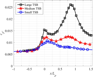
A streamwise plot of the fluctuating pressure coefficient ${c_{p^{\prime }}}=2p_{rms}/\rho U_{ref}^2$, defined as the standard deviation of the fluctuating wall pressure normalized by the incoming dynamic pressure, is shown in figure 9 as a function of $x/L_p$. For the three flows the distribution is bi-modal, with a first maximum at $x/L_p \simeq 0$ and a second at $x/L_p \simeq 0.75$, though for the Small TSB this second maximum is almost non-existent. The pressure fluctuations clearly increase with the size of the TSB, especially near the second maximum at $x/L_p \simeq 0.75$. Coincidentally, for the Medium TSB both maxima have essentially the same value, whereas the second maximum is clearly larger than the first for the Large TSB, and respectively smaller for the Small TSB. A bi-modal distribution of ${c_{p^{\prime }}}$ was also observed in the DNS of Na & Moin (Reference Na and Moin1998b) and Abe (Reference Abe2017). The latter author investigated the influence of the TSB size on the wall-pressure fluctuations at $Re_{\theta }=300$ and showed that consistently with the present results, fluctuations increase with the bubble size, particularly in the region of the second maximum. The large TSB in Abe (Reference Abe2017) has both maxima at approximately ${c_{p^{\prime }}}=0.20$, compared to ${c_{p^{\prime }}} \simeq 0.12$ for our Medium TSB. At $Re_{\theta }=900$ the second maximum for the large TSB in Abe (Reference Abe2017) remains at ${c_{p^{\prime }}} \simeq 0.20$ whereas the first decreases to ${c_{p^{\prime }}} \simeq 0.13$, thereby implying a significant Reynolds number effect. The first maximum in Na & Moin (Reference Na and Moin1998b) is at ${c_{p^{\prime }}} \simeq 0.13$ and their second maximum at ${c_{p^{\prime }}} \simeq 0.18$, which corresponds to a distribution between our Medium and Large TSBs.

Figure 9. Fluctuating wall-pressure coefficient ${c_{p^{\prime }}}$ measured on the test-section centreline for the three TSBs.

The wall-pressure fluctuations are investigated in the frequency domain in figure 10. The plot on the top of the figure shows the power spectral density (PSD) calculated at $x/L_p =0$ and $x/L_p = 0.75$, i.e. the locations of the two maxima of figure 9, for the three separation bubbles. For reference, the PSD of pressure fluctuations in the incoming ZPG turbulent boundary layer is also provided. At $x/L_p = 0$, the PSD levels of the three TSBs are essentially the same for frequencies above 10 Hz. For $f<10$ Hz, however, the amount of energy in the signals is larger for a larger bubble, consistently with the ${c_{p^{\prime }}}$ distributions of figure 9. This shows that differences in the level of pressure fluctuations at $x/L_p \simeq 0$ are caused by low-frequency unsteady phenomena. Note also that the PSD levels in the three TSBs are higher than those of the incoming boundary layer in the complete frequency range that was investigated, which implies that even without the low-frequency contribution, a peak in ${c_{p^{\prime }}}$ would be observed near $x/L_p = 0$. At $x/L_p = 0.75$, the shape of the PSDs is different. There is still an increase in energy with TSB size at low frequency ($f<10$ Hz), however, the major difference occurs for frequencies between 10 Hz and 300 Hz, with the Large TSB again showing a stronger increase in energy compared to the others. For frequencies above 300 Hz the PSD levels decrease, even to values lower than in the ZPG boundary layer. These observations imply that the energy of the pressure fluctuations is essentially shifted from a broadband character in the incoming attached boundary layer to low ($f<10$ Hz) and medium ($10<f<300$ Hz) frequencies under the separation bubbles, with the lower frequencies increasing earlier than the medium frequencies when moving in the streamwise direction.

Figure 10. (a) Power spectral density of wall-pressure fluctuations at $x/L_p \simeq 0$ (solid lines) and $x/L_p \simeq 0.75$ (dash-dot lines). Black: Large TSB; red: Medium TSB; blue: Small TSB. Grey dashed line is the PSD measured in the incoming boundary layer upstream of separation ($x=1.05$ m). (b) Pre-multiplied PSD normalized by the signal's variance, same colour coding as above.

Figure 10(b) shows the same data but plotted as the PSD pre-multiplied by the frequency and normalized by each signal's variance ($f \times PSD(f) / \sigma ^2_{p'}$). This representation is useful because it shows the distribution of energy as the area under each curve in a semi-logarithmic plot since $\int _0^{\infty } PSD(f)\,\textrm {d}f = \int _0^{\infty } f \times PSD(f) \,\textrm {d}\ln (f)$. In this plot the low- and medium-frequency ranges are particularly obvious. At $x/L_p = 0$ the energy is concentrated in the low-frequency ($f<10$ Hz) as well as the high-frequency ($f>100$ Hz) range, with almost nothing in between. For the Large TSB there is almost the same amount of energy in the low-frequency as in the high-frequency range but for the Small and Medium TSBs, the high-frequency part is dominant. It is noteworthy that at $x/L_p = 0$, the pre-multiplied PSDs are cut-off by the anti-aliasing filter of the data acquisition card at $f\simeq 1$ kHz. This implies that the wall-pressure fluctuation levels are likely to be underestimated in the upstream part of our TSBs due to the limited temporal resolution of the pressure taps. Indeed, the review of Bull (Reference Bull1996) indicates an expected level of ${c_{p^{\prime }}}=0.009$ in our turbulent ZPG boundary layer at $Re_\theta = 5000$ (see his figure1 with $u_{\tau } = 1\ \textrm {m}\ \textrm {s}^{-1}$ and $\delta =28$ mm), which is larger than ${c_{p^{\prime }}}=0.006$ obtained in the present experiment. This underestimation of ${c_{p^{\prime }}}$, however, would only be limited to the incoming ZPG boundary layer and the very upstream part of our TSBs where the forward-flow fraction remains close to 100 % (see figure 7) and where the high-frequency pressure fluctuations are still significant (the effect of this limitation in our experimental technique will be further discussed in relationship with figure 15). In contrast to the spectra obtained a $x/L_p = 0$, those calculated at $x/L_p = 0.75$ show that almost all the energy of the fluctuating pressure is concentrated in a medium-frequency range, between $f \simeq 10$ Hz and $f \simeq 300$ Hz. The characteristic frequencies of these fluctuations, defined as the centre of the medium-frequency peak in the semi-logarithmic pre-multiplied representation, is approximately 25, 30 and 80 Hz for the Large, Medium and Small TSBs, respectively. The pre-multiplied PSDs further show than the frequency resolution of the measurements is more than adequate at these streamwise positions.

We now turn our attention to the mechanisms causing the low- and medium-frequency pressure fluctuations, beginning with the latter. In the case of the Large TSB, Mohammed-Taifour & Weiss (Reference Mohammed-Taifour and Weiss2016) showed that the pressure fluctuations near the second maximum of the ${c_{p^{\prime }}}$ distribution in figure 9 are caused by the convection of large-scale, roller-type structures originating in the shear layer via a Kelvin–Helmholtz instability and subsequently shed downstream of the bubble. This medium-frequency unsteadiness was therefore called the ‘shedding mode’ of the TSB. To illustrate the convective nature of this unsteady mode, two-point cross-correlation contours of the wall-pressure and velocity fluctuations measured on the test-section centreline are presented in figure 11 for the case of the Medium TSB. The image on the top of the figure was obtained using a reference pressure transducer at a fixed position of $x_{ref}/L_p=0.69$ (which corresponds to $x_{ref}=2.05$ m), and a second pressure transducer covering the range $0.1<x/L_p<1.3$. On the bottom image, velocity cross-correlations were extracted from the PIV data along the centre of the shear layer defined by the loci of maximum $u'^2$, with again a reference position at $x_{ref}=2.05$ m. The streamwise extent of the cross-correlation plots is smaller for the velocity data because of the limited PIV field of view.

Figure 11. Contour of wall-pressure (a) and streamwise velocity (b) two-point cross-correlation along the test-section centreline (Medium TSB). The reference position is at $x_{ref} = 2.05$ m. The black dashed line is the slope corresponding to a convection velocity $U_c/U_{ref}=0.33$ (Na & Moin Reference Na and Moin1998b).

Both the pressure and velocity cross-correlation contours show a clear ridge indicating disturbances with a convective nature. The average slope of this ridge is a measure of the convection velocity of the large-scale structures, which is seen to be very close to the value of $U_c/U_{ref}=0.33$ suggested by Na & Moin (Reference Na and Moin1998b) and plotted as a dashed line in figure 11. The same analysis was performed on data from all three TSBs and essentially shows very similar results, including an almost constant value of the convection velocity. This is the case even for the Small TSB which does not feature any region of mean back flow. Thus, the occurrence of a convective shedding mode does not require the flow to reach an average separated state, but merely the presence of inflectional velocity profiles from the APG. This is consistent with the idea of coherent structures generated by Kelvin–Helmholtz instabilities in a manner similar to what is observed in turbulent mixing layers, as argued in Winant & Browand (Reference Winant and Browand1974). Nevertheless, a larger separation bubble clearly produces shedding with a larger pressure signature, as evidenced by figure 9. This is attributed to larger coherent structures when the shear layer separates further away from the wall.

In contrast to the convective medium-frequency shedding mode, the low-frequency unsteadiness in the Large TSB was shown to be linked to a large-scale contraction and expansion, dubbed ‘breathing’, of the whole separation bubble (Weiss et al. Reference Weiss, Mohammed-Taifour and Schwaab2015). In particular, this breathing motion was well illustrated by the first proper orthogonal decomposition (POD) mode of the fluctuating velocity field (Mohammed-Taifour & Weiss Reference Mohammed-Taifour and Weiss2016). The relevance of the first POD mode for studies of large-scale unsteadiness in TSBs was recently confirmed by Fang & Tachie (Reference Fang and Tachie2019), who demonstrated that its time coefficient $a^1(t)$ is well synchronized with the time history of the total reverse-flow area $A_{xy}(t) = \iint _{x,y} -\textrm {sign}(U(t)) \,\textrm {d}x\,\textrm {d}y$. The latter indicator has been used by Pearson, Goulart & Ganapathisubramani (Reference Pearson, Goulart and Ganapathisubramani2013) and Wu et al. (Reference Wu, Meneveau and Mittal2020) as a simple parameter that measures the large-scale unsteadiness in separation bubbles. $A_{xy}$ is most relevant for TSBs that feature large regions of instantaneous back flow at all time. This is the case in our Medium and Large TSBs, but not in our Small TSB. Therefore, in order to provide a more widely applicable indicator of large-scale unsteadiness, we introduce the quantity $B_{xy}(t) = \iint _{x,y} ({U_{ref}}-U(t)) \,\textrm {d}x\,\textrm {d}y$, which essentially measures the instantaneous size of the decelerated flow region even in the absence of back flow. The time trace of $B_{xy}(t)$ is compared to the time coefficient $a^1(t)$ of the first POD mode of the longitudinal velocity field in figure 12. While these particular data were measured on the centreline plane of our Medium TSB, similar results were obtained for all three separation bubbles. The synchronization between the two signals is remarkable, which further consolidates the first POD mode as a relevant indicator of the breathing motion.

Figure 12. Time history of the first POD mode $a^1(t)$ and the decelerated-flow indicator $B_{xy}(t)$ on the test-section centreline, Medium TSB.

A snapshot POD analysis was performed on all three TSBs by using the PIV field of view closest to the centre of each bubble. The POD spectra showing the repartition of the longitudinal turbulent kinetic energy across the modes are shown in figure 13 for two sets of velocity data: the original (unfiltered) longitudinal velocity and the velocity digitally high-pass filtered at $f>10$ Hz. Looking at the original velocity data first, it can be seen that the first POD mode is significantly more energetic than the second, with a difference of approximately 5 %, 10 % and 15 % between first and second POD modes for the Small, Medium and Large TSB, respectively. Since the first POD mode is representative of the breathing motion, this shows that the low-frequency breathing is more pronounced for a larger TSB, which is consistent with the Fourier analysis of figure 10 where the low-frequency pressure signature is clearly larger for a larger separation bubble. This analysis is confirmed by looking at the POD spectra obtained from the velocity fields high-pass filtered above 10 Hz: in this case there is only a few percentage points of difference between the first and second POD modes, irrespective of the size of the TSB. This confirms that for $f<10$ Hz, the flow behaves somewhat differently than at higher frequencies.

Figure 13. POD spectrum of longitudinal velocity fluctuations in the three TSBs (snapshot POD calculated from a field of view central to each separation bubble). Black stars: POD calculated on original velocity data. Red squares: POD calculated on data high-pass filtered at 10 Hz.

The first three POD modes of the longitudinal velocity field in the Medium TSB are shown in figure 14, again for the original velocity field and the high-pass filtered field ($f>10$ Hz). Note that similar results were obtained for all three separation bubbles. In the case of the original velocity, the first mode appears to be of uniform sign, and represents a contraction and expansion of the complete TSB since, when multiplied by its time coefficient $a^1(t)$, it exhibits a structure that effectively enlarges or shrinks the separation bubble (Mohammed-Taifour & Weiss Reference Mohammed-Taifour and Weiss2016; Fang & Tachie Reference Fang and Tachie2019). In contrast, the subsequent modes show a change of sign, which is indicative of the convection of turbulent structures in the flow (Rajaee, Karlsson & Sirovich Reference Rajaee, Karlsson and Sirovich1994; Weiss Reference Weiss2019). When only frequencies above 10 Hz are considered in the POD analysis, the uniform character of the first mode disappears and the convective nature of the fluctuations appears already in the first mode. Again, this is fully consistent with the spectral analysis of the pressure data presented in figure 10 and confirms the presence of a low-frequency breathing mode for frequencies below 10 Hz, the intensity of which increases with the size of the TSB. This effect of TSB size is consistent with the recent DNS of Wu et al. (Reference Wu, Meneveau and Mittal2020), who observed a much larger variation of the reverse-flow area $A_{xy}(t)$ for a large TSB generated with a suction-only boundary condition than for a smaller TSB obtained using suction and blowing.

Figure 14. First, second and third POD modes of longitudinal velocity in the Medium TSB (arbitrary scale). (a) POD calculated on original velocity data. (b) POD calculated on data high-pass filtered at 10 Hz.

Based on these new results, it would be of interest to plot the streamwise distribution of the fluctuating pressure coefficient for frequencies above 10 Hz only, as this would remove the pressure signature of the low-frequency breathing motion. This is done in figure 15, where the most interesting result is remarkably that the three curves now see their first maximum collapse on each other and exhibit approximately the same amplitude of ${c_{p^{\prime }}} \simeq 0.01$ at $x/L_p = 0.1$. This streamwise position corresponds to the end of the strong adverse pressure-gradient zone and the beginning of the flow detachment from the wall, with approximately 10 % of reverse flow (figure 7). It also corresponds very well to the position of the first maximum of ${c_{p^{\prime }}}$ observed in the direct simulations of Na & Moin (Reference Na and Moin1998b) and Abe (Reference Abe2017). From the spectral plots of figure 10 it is obvious that at $x/L_p \simeq 0.1$, the pressure fluctuations are mostly confined to the low- and high-frequency parts of the spectrum. Removing the low-frequency breathing then implies that only the high-frequency turbulent motions are now taken into account. The rise in ${c_{p^{\prime }}}$ up to $x/L_p = 0.1$ is then interpreted as the effect of the adverse pressure gradient on the turbulent structures responsible for pressure fluctuations in the attached boundary layer, while the decrease of ${c_{p^{\prime }}}$ beyond $x/L_p = 0.1$ corresponds to the lifting of those structures away from the test surface in the early stages of detachment. This is consistent with the wall-normal profiles of pressure fluctuations shown by Na & Moin (Reference Na and Moin1998b), as seen in their figure 13, where the position of maximum pressure fluctuations is shown to move away from the wall at the very end of the pressure ramp. Furthermore, given that the APG imposed on the incoming turbulent boundary layer is essentially the same for all of our three TSBs (figure 1), it would be expected that the turbulent fluctuations react to the APG in approximately the same way upstream of the mean detachment. This is indeed confirmed by the filtered ${c_{p^{\prime }}}$ distributions of figure 15.

Figure 15. Fluctuating wall-pressure coefficient ${c_{p^{\prime }}}$ measured on the test-section centreline for the three TSBs. Black: Large TSB, red: Medium TSB, blue: Small TSB. Dashed lines are unfiltered values from figure 9 while solid lines are high-pass filtered above 10 Hz. Solid green line are high-pass filtered data from flush-mounted pressure transducer ($f_s=16$ kHz), Large TSB.

A noteworthy feature that was previously mentioned in connection with figures 9 and 10 is the limited sampling frequency ($f_s=2$ kHz) of the fluctuating wall-pressure measurements caused by the use of regular pressure taps instead of a frequency-calibrated pinhole. It was argued that the effect of this limited bandwidth would only be felt in the ZPG region and the most upstream part of the pressure-gradient zone. To investigate this in more details, dedicated measurements were performed in the Large TSB using a flush-mounted pressure transducer at a higher sampling frequency of $f_s=16$ kHz. The results from figure 15 (green solid line) show that taking into account a larger frequency band increases ${c_{p^{\prime }}}$ up to 0.010 in the ZPG region, which is very close to the value of 0.009 expected from the review of Bull (Reference Bull1996). The ${c_{p^{\prime }}}$ level then slightly increases at $x/L_p \simeq 0.1$ and decreases afterwards, following the values obtained at a lower sampling frequency. This confirms that the wall-pressure measurement set-up is indeed adequate within the separation bubbles and demonstrates that the observation of a well-defined local maximum of ${c_{p^{\prime }}}$ depends in fact on the selection of a specific frequency band.

In summary, the results presented in this section confirm the presence of a low-frequency unsteadiness whose amplitude appears to depend on the size of the TSB, with the largest pressure signature observed for the largest TSB. For the latter, Mohammed-Taifour & Weiss (Reference Mohammed-Taifour and Weiss2016) demonstrated that this unsteady character of pressure-induced separation bubbles was inherently linked to a contraction and expansion motion of the entire recirculation region. Removing this low-frequency contribution collapses the first maximum of the fluctuating pressure coefficient to a single value for all three separation bubbles. Interestingly, the ${c_{p^{\prime }}}$ distributions remain bi-modal after removal of the low-frequency contribution, which is consistent with the DNS results of Na & Moin (Reference Na and Moin1998b) and Abe (Reference Abe2017), who did not resolve the low-frequency fluctuations. This shows that the first maximum of ${c_{p^{\prime }}}$ is in fact the result of two separate phenomena: on the one hand, the signature of the low-frequency breathing motion, mostly apparent at the position of maximum adverse pressure gradient, and on the other hand the increase in high-frequency pressure fluctuations caused by the turbulent structures submitted to an APG and their subsequent lift-off from the wall. This reconciles the DNS results of Na & Moin (Reference Na and Moin1998b) and Abe (Reference Abe2017) with the conclusions of Weiss et al. (Reference Weiss, Mohammed-Taifour and Schwaab2015) and Mohammed-Taifour & Weiss (Reference Mohammed-Taifour and Weiss2016) obtained from observations of the Large TSB only.

3.3. Velocity statistics and scaling of pressure fluctuations

In this section we investigate the velocity statistics obtained by PIV on the test-section centreline and the scaling of wall-pressure fluctuations with the Reynolds shear stresses and wall-normal stresses, as suggested by the previous works of Simpson et al. (Reference Simpson, Ghodbane and McGrath1987), Na & Moin (Reference Na and Moin1998b), Ji & Wang (Reference Ji and Wang2012) and Abe (Reference Abe2017).

Contour plots of the normalized turbulent streamwise $\overline {u'u'}/U_{ref}^2$, wall-normal $\overline {v'v'}/U_{ref}^2$ and shear $-\overline {u'v'}/U_{ref}^2$ stresses, are shown in figure 16. Note that the colour bars were adjusted to make the Small and Medium TSBs stand out more easily on the figure since the large bubble exhibits much higher values for all three Reynolds stresses. Therefore, the dark red areas in the third column are fully saturated. Nevertheless, the contours are consistent between the three separation bubbles and the amplitude of each turbulent stress generally increases with the size of the bubble. The loci of maximum stresses also tend to move away from the test surface as the TSB size grows. In the streamwise direction, $\overline {u'u'}/U_{ref}^2$ starts increasing slightly upstream of $x/L_p=0$ and reaches its maximum near $x/L_p=0.2$ (see also figure 17), which is consistent with the contours shown in Na & Moin (Reference Na and Moin1998a) and those of Coleman et al. (Reference Coleman, Rumsey and Spalart2018); see figure 4 for a direct comparison between their case C and our Medium TSB. The wall-normal and shear stresses behave differently and increase from $x/L_p\simeq 0$ until the end of the PIV field of view. These contours are again close to those of Coleman et al. (Reference Coleman, Rumsey and Spalart2018), e.g. figure 4, but differ somewhat from those of Na & Moin (Reference Na and Moin1998a) and Abe (Reference Abe2017), who observed a decrease of $\overline {v'v'}/U_{ref}^2$ and $-\overline {u'v'}/U_{ref}^2$ near the middle of their TSBs. This bi-modal distribution of the turbulent stresses is not observed in our data, except perhaps in the case of the Large TSB, where the Reynolds shear stress is seen to decrease slightly at $x/L_p \simeq 0.2$ compared to more upstream and downstream positions (see also figure 17). This aspect will be discussed further below.

Figure 16. Contour plot of (a) $\overline {u'u'}/U_{ref}^2$, (b) $\overline {v'v'}/U_{ref}^2$ and (c) $-\overline {u'v'}/U_{ref}^2$ for the three TSBs. The black dash-dot lines are the loci of the maximum stresses. Black rectangles near the wall are caused by limitations in optical access. The black squares, crosses and triangles denote ID or CR ($\gamma =99$ %), intermittent transitory detachment or reattachment ($\gamma =80$ %) and transitory detachment or reattachment ($\gamma =50$ %), respectively.

Figure 17. Maxima of (a) $\overline {u'u'}/U_{ref}^2$, (b) $\overline {v'v'}/U_{ref}^2$ and (c) $-\overline {u'v'}/U_{ref}^2$ for the three TSBs. Solid lines: original (unfiltered) data; dashed-dotted lines: data (high-pass) filtered at 10 Hz; black dotted lines are expected ZPG values from Fernholz & Finley (Reference Fernholz and Finley1996), for reference.

The maxima of the three normalized turbulent stresses are plotted as a function of the streamwise position in figure 17. Given the relevance of the low-frequency contribution $f<10~Hz$ in the pressure fluctuations, the high-pass-filtered stresses are presented as well. It can be seen that removing the low-frequency contribution has the largest effect on the streamwise stresses, particularly near the middle of the TSB. The effects of filtering on the wall-normal and shear stresses are less significant and confined to the downstream part of the separation bubbles, where the stresses are themselves larger. For all stresses the largest difference between filtered and non-filtered data is seen on the Large TSB, which is consistent with the high-pass filtering of the pressure fluctuations (see figures 9 and 15). Note that high-pass filtering the velocity data enables a better comparison with existing DNS data, which, by current design, excludes low-frequency fluctuations. For example, the lowest Strouhal number resolved in the DNS of Abe (Reference Abe2017) is $St=f L_b / U_{ref} \simeq 0.13$, which corresponds to a dimensional frequency of approximately 8 Hz in our Large TSB. Regardless of the bandwidth taken into account, figure 17 shows a strong increase of $-\overline {u'v'}_{max}/U_{ref}^2$ and $\overline {v'v'}_{max}/U_{ref}^2$ in the reattachment region of the Large TSB, which is coincident with the large values of ${c_{p^{\prime }}}$ in this region (figure 9). This indicates that the strong pressure signature of the shedding mode in the Large TSB is directly related to larger turbulent stresses, in agreement with the experimental results of Simpson et al. (Reference Simpson, Ghodbane and McGrath1987) and the DNS of Na & Moin (Reference Na and Moin1998b).

Also included in figure 17 are the values of the maximum turbulent stresses expected in a canonical ZPG turbulent boundary layer at $Re_\theta =5000$, obtained from the review of Fernholz & Finley (Reference Fernholz and Finley1996). It can be seen that at the most upstream positions, our measured values are generally lower than the expected ZPG levels, with an underestimation of approximately 50 % for $\overline {u'u'}/U_{ref}^2$, 15 % for $\overline {v'v'}/U_{ref}^2$ and 20 % for $-\overline {u'v'}/U_{ref}^2$. This can be explained by the fact that at this Reynolds number, the wall-normal position of maximum stress is expected at 0.22, 5.4 and 2.9 mm for $\overline {u'u'}/U_{ref}^2$, $\overline {v'v'}/U_{ref}^2$ and $-\overline {u'v'}/U_{ref}^2$, respectively (Fernholz & Finley Reference Fernholz and Finley1996). Given our spatial resolution of 0.55 mm and the inherent limitations of PIV measurements very near the wall, this difference is not surprising. Nevertheless, this underestimation should only be significant in the most upstream part of the TSBs (see the favourable comparison between hot-wire and PIV measurements of $\overline {u'u'}/U_{ref}^2$ in Mohammed-Taifour & Weiss (Reference Mohammed-Taifour and Weiss2016) for the case of the Large TSB).

In analysing figure 17, it is of interest to compare with the results of Abe (Reference Abe2017), who also investigated the effect of varying the TSB size on the streamwise distributions of $-\overline {u'v'}_{max}/U_{ref}^2$ and $\overline {v'v'}_{max}/U_{ref}^2$. This was done by varying the maximum transpiration velocity $[V_{top}/U_{ref}]_{max}$ at a constant Reynolds number $Re_{\theta }=300$. Consistently with our data, both $-\overline {u'v'}_{max}/U_{ref}^2$ and $\overline {v'v'}_{max}/U_{ref}^2$ were shown to increase with the size of the bubble near the reattachment. The increase was more moderate closer to the detachment, however, and $-\overline {u'v'}_{max}/U_{ref}^2$ even decreased near the middle of the TSB when the bubble got larger. This was attributed, according to Abe, to a negative TKE production rate near the top of the bubble that arises because of the rapid switch between positive and negative vertical transpiration velocity. As $[V_{top}/U_{ref}]_{max}$ is increased to generate a larger TSB, the production term becomes more negative and $-\overline {u'v'}_{max}/U_{ref}^2$ decreases (Abe Reference Abe2017). This argument is consistent with the small decrease of $-\overline {u'v'}_{max}/U_{ref}^2$ that is observed near $x/L_p=0.2$ for our Large TSB only.

Further comparisons between our experimental data (Medium and Large TSB) and the distributions of $-\overline {u'v'}_{max}/U_{ref}^2$ and $\overline {v'v'}_{max}/U_{ref}^2$ from other sources are presented in figure18. Starting with $-\overline {u'v'}_{max}/U_{ref}^2$, it can be seen that our Medium TSB and the Coleman et al. (Reference Coleman, Rumsey and Spalart2018) case C stand out by showing a monotonic increase with $x/L_p$. All other distributions, including CRS case A, show a clear minimum between $x/L_p = 0.3$ and $x/L_p=0.7$. As already discussed above, this minimum is attributed to the larger value of $[V_{top}/U_{ref}]_{max}$ for large separation bubbles, which leads to smaller TKE production rate when $[V_{top}/U_{ref}](x)$ crosses zero and hence to a decrease of $-\overline {u'v'}/U_{ref}^2$ below the top of the bubble (Abe Reference Abe2017; Coleman et al. Reference Coleman, Rumsey and Spalart2018). For our Large TSB the value of $[V_{top}/U_{ref}]_{max}$ is large enough to show a small dip in $-\overline {u'v'}_{max}/U_{ref}^2$ near $x/L_p=0.2$, in a manner very similar to the Patrick (Reference Patrick1987) data. The values of $-\overline {u'v'}_{max}/U_{ref}^2$ obtained by Na & Moin (Reference Na and Moin1998a), Abe (Reference Abe2017) (cases SB2 and LB) and Coleman et al. (Reference Coleman, Rumsey and Spalart2018) (case A) for $x/L_p<0.5$ are relatively large compared to our data, to the Coleman et al. (Reference Coleman, Rumsey and Spalart2018) case C and to Patrick (Reference Patrick1987). This is attributed to a lower Reynolds number for those former cases. Indeed, the results of Abe (Reference Abe2017) clearly indicate a decrease of $-\overline {u'v'}_{max}/U_{ref}^2$ (and to a lesser extent $\overline {v'v'}_{max}/U_{ref}^2$) when the Reynolds number increases, which is consistent with figure 18. The combined effects of a larger $[V_{top}/U_{ref}]_{max}$ and a larger Reynolds number, which have opposite effects on the value of $-\overline {u'v'}_{max}/U_{ref}^2$ for $x/L_p<0.5$, may also explain why the Patrick (Reference Patrick1987) data are very close to our Large TSB. Moving on to the downstream half of the bubbles ($x/L_p>0.5$) indicates that $-(\overline {u'v'})_{max}$ essentially increases with the size of the TSBs and, consistently with the values of $H_b/L_b$ shown in table 1, the Patrick (Reference Patrick1987) data show the largest value of $-\overline {u'v'}_{max}/U_{ref}^2$ near reattachment.

Figure 18. Maxima of $-\overline {u'v'}/U_{ref}^2$ (a) and $\overline {v'v'}/U_{ref}^2$ (b) for current and existing TSB data. Current data high-pass filtered at 10 Hz.

The distributions of $\overline {v'v'}_{max}/U_{ref}^2$ (bottom of figure 18) are generally consistent with those of $-\overline {u'v'}_{max}/U_{ref}^2$ in as much as a larger TSB generates a larger stress in the downstream half of the bubble. The results of Abe (Reference Abe2017) (cases SB2 and LB) and Coleman et al. (Reference Coleman, Rumsey and Spalart2018) (case A) show a bi-modal distribution with a minimum of $\overline {v'v'}_{max}/U_{ref}^2$ near $x/L_p=0.5-0.6$, while the others show a monotonic increase with a plateau near $x/L_p=0.3$ (note that Na & Moin (Reference Na and Moin1998a) did not publish their distribution of $\overline {v'v'}_{max}/U_{ref}^2$). This difference is attributed to the combined effect of Reynolds number and TSB size, where a larger Reynolds number tends to bring the first peak down, and a larger TSB the second peak up. Note that for a large bubble, the streamwise increase of $\overline {v'v'}/U_{ref}^2$ tends to start more upstream than $-\overline {u'v'}/U_{ref}^2$ (see figure 16), which explains the large value of $\overline {v'v'}_{max}/U_{ref}^2$ downstream of $x/L_p=0.2$ for the Patrick (Reference Patrick1987) fairly large TSB.

The scaling of the wall-pressure fluctuations with the maximum Reynolds shear stresses ${-\rho \overline {u'v'}_{max}}$ and the wall-normal stresses ${\rho \overline {v'v'}_{max}}$ is presented in figure 19. The high-pass filtered results are used for our data, which collapses the values of $p_{w\ {rms}}$ near $x/L_p=0$ by removing the effect of the low-frequency breathing motion. As already mentioned above, this enables a more rigorous comparison with existing DNS data. Also, the expected ZPG levels obtained using the wall-pressure data collected by Bull (Reference Bull1996) and the turbulence data reviewed by Fernholz & Finley (Reference Fernholz and Finley1996) are included in the figure. The measured distributions of $p_{w\ {rms}}/{-\rho \overline {u'v'}_{max}}$ and $p_{w\ {rms}}/{\rho \overline {v'v'}_{max}}$ are seen to converge towards these levels, which gives confidence in the results despite the experimental limitations observed in the most upstream part of the TSBs.

Figure 19. Scaling of wall-pressure fluctuations with ${-\rho \overline {u'v'}_{max}}$ (a) and ${\rho \overline {v'v'}_{max}}$ (b). Current data high-pass filtered at 10 Hz. Error bars were computed by propagating the uncertainties quantified in § 2.2.

In a separating turbulent boundary layer, Simpson et al. (Reference Simpson, Ghodbane and McGrath1987) experimentally found that $p_{w\ {rms}}/{-\rho \overline {u'v'}_{max}}$ increases up to a value of approximately 4 near the detachment and decreases afterwards. This is consistent with the behaviour obtained in the present experiment, though our Large TSB shows a larger maximum value of $p_{w\ {rms}}/-\rho \overline {u'v'}_{max} = 5$ near $x/L_p=0.2$. The Na & Moin (Reference Na and Moin1998b) and Abe (Reference Abe2017) data show essentially the same trend, but with slightly lower values. Generally speaking, both scalings succeed very well in collapsing the large differences in ${c_{p^{\prime }}}$ observed near reattachment for the three TSBs (figure 15), though the scaling with ${\rho \overline {v'v'}_{max}}$ is perhaps better over a longer distance. Nevertheless, neither scaling law is fully satisfactory over the full length of the separation bubbles since the value of $p_{w\ {rms}}/{-\rho \overline {u'v'}_{max}}$ and $p_{w\ {rms}}/{\rho \overline {v'v'}_{max}}$ is not constant over $x$. This indicates that the mechanisms leading to wall-pressure fluctuations are not identical near the detachment and near the reattachment, which is consistent with the spectral analysis of figure 10 showing a separation of scales into low-frequency breathing, medium-frequency shedding and high-frequency turbulent fluctuations. Note also that using unfiltered data would reduce the quality of both scalings by increasing the discrepancies between the three TSBs at $x/L_p \simeq 0$ (Le Floc'h et al. Reference Le Floc'h, Mohammed-Taifour, Dufresne and Weiss2019). This indicates that the low-frequency breathing motion does not appear to be directly related to turbulent stresses.

3.4. Three-dimensional effects

In this last section we take a look at the pressure fluctuations and their scaling across the span of the wind tunnel, as the discussion in § 3.1 revealed the presence of secondary flows affecting a large portion of the test section.

The spanwise variation of the fluctuating pressure coefficient ${c_{p^{\prime }}}$ is presented in figure 20 for the three separation bubbles. Apart from small imperfections, all curves are essentially symmetric with respect to the test-section centreline, but show significant variations of amplitude across the span. The spanwise effects appear to be stronger near reattachment ($x/L_p=1$) than near detachment ($x/L_p = 0$), which is consistent with the global character of the average flows: as illustrated by the RANS results of figure 6, the corner vortices generated by secondary flows on the sidewalls slowly increase in size as the flow develops downstream of the mean separation, which implies a larger spanwise ‘contamination’ as the flow proceeds towards the exit of the test section (Le Floc'h et al. Reference Le Floc'h, Mohammed-Taifour, Dufresne and Weiss2018). Furthermore, the three-dimensional effects appear to be strongest for the Medium TSB since at $x/L_p \simeq 1$, ${c_{p^{\prime }}}$ is only approximately constant in a narrow region near the test-section centreline ($\left \lvert z ^*\right \rvert <1/6$). For the Small and Large TSBs, the quasi-two-dimensional extent of the flow is somewhat larger, with pressure fluctuations that are essentially constant over a third of the span ($\left \lvert z ^*\right \rvert <1/3$). Interestingly, the spanwise extent of the quasi-two-dimensional regions revealed by the pressure fluctuations is slightly smaller than that observed in the oil-film visualizations of figure 5. Defining the width $w_{2D}$ as the approximate extent of the quasi-two-dimensional flow observed from figure 20, the values of $w_{2D}/L_p$ are 0.43, 0.16 and 0.24 for the Small, Medium and Large TSBs, respectively. As can be seen in table 1, this is smaller than the spanwise extent of most existing numerical simulations.

Figure 20. Normalized fluctuating pressure coefficient measured across the test section's span.

In order to investigate three-dimensional effects in more details, further PIV measurements were performed in the Medium TSB. The field of view was limited to $0.2<x/L_p<0.6$ but the cameras were translated in the spanwise direction in order to image the separation bubble at 5 positions across the span of the test section. Measurements were only taken on one side of the test section, given the appropriate symmetry of the oil-film visualizations in figure 5 and of the pressure fluctuations in figure 20. The height of the local recirculation regions, identified by the mean dividing streamline $\psi =0$ calculated at each spanwise position, is shown in figure 21. It can be seen that the separation bubble is strongly distorted across the span, with a larger bubble height near the sidewall than near the centreline. This distortion is caused by the corner vortices discussed in § 3.1. Near the sidewalls, the larger recirculation region increases the wall-pressure and the corresponding velocity fluctuations in a manner consistent with the increase of fluctuations with TSB size, as described in §§ 3.2 and 3.3.

Figure 21. Mean dividing streamline ($\psi =0$) for different spanwise positions, Medium TSB.

Nevertheless, the scaling of wall-pressure fluctuations proposed above appears to hold in the spanwise direction. Figure 22 shows the spanwise variation of ${c_{p^{\prime }}}$, $-\overline {u'v'}_{max}/U_{ref}^2$ and $\overline {v'v'}_{max}/U_{ref}^2$ at $x/L_p =0.45$. Both turbulent stresses display a similar trend as the pressure fluctuations, which leads to a nearly constant value of $p_{w\ {rms}}/{-\rho \overline {u'v'}_{max}}$ and $p_{w\ {rms}}/{\rho \overline {v'v'}_{max}}$ across the span. We conclude that although corner effects strongly distort the average flow, the unsteady character of the TSBs and the scaling of the pressure fluctuations remain relatively unaffected. While the spanwise PIV measurements were only performed on the Medium TSB, where three-dimensional effects are the strongest, it is reasonable to expect a similar behaviour for the small and large separation bubbles as well. Therefore, although the separation bubbles generated in our wind tunnel are necessarily unique in as much as they depend on the test-section geometry, the flow physics investigated in this work appears to be of general nature.

Figure 22. (a) Spanwise distributions of ${c_{p^{\prime }}}$, $-\overline {u'v'}_{max}/U_{ref}^2$ and $\overline {v'v'}_{max}/U_{ref}^2$. (b) Spanwise distributions of $p_{w\ {rms}}/{-\rho \overline {u'v'}_{max}}$ and $p_{w\ {rms}}/{\rho \overline {v'v'}_{max}}$. Medium TSB at $x/L_p =0.45$.