2.0 TIME-CONTINUOUS NON-LINEAR AND LINEAR STATE-SPACE SYSTEMS

In this work, the unsteady Euler or RANS equations are solved using a standard Jameson cell-centred finite-volume scheme code^{(Reference Jameson, Schmidt and Turkel11,Reference Kroll and Jain12)} that is modified to be time accurate and allows moving meshes^{(Reference Gaitonde13-Reference Arnone, Liou and Povinelli15)}. After spatial discretisation, the CFD equations for the motion about a non-linear baseline Euler or RANS solution can be written^{(Reference Griffiths10)} in non-linear state space form as:

(1) $$\begin{eqnarray} \frac{{\rm d}\mathbf {x}\left(t\right)}{{\rm d}t} & = & \mathbf {f}\left(t,\mathbf {x}\left(t\right),\mathbf {u}\left(t\right)\right),\nonumber \\ \mathbf {y}\left(t\right) & = & \mathbf {h}\left(t,\mathbf {x}\left(t\right),\mathbf {u}\left(t\right)\right), \end{eqnarray}$$

where (u) is the input vector, (x) is the state vector and (y) is the output vector, containing quantities of interest such as changes to force coefficients or surface pressures. For example, for an aerofoil undergoing linearised perturbations in pitch (Δα), heave (Δh) and flap (Δδ) motions; where the outputs of interest are the changes to the integrated coefficients of lift (ΔC_l ), drag (ΔC_d ), pitching moment (ΔC_m ) and flap hinge moment (ΔC_h ) compared to the initial mean values obtained from the steady non-linear CFD solver, then

(2) $$\begin{equation} \begin{array}{r@{\quad}l@{\quad}l}\mathbf {u}&=&\left[\Delta \alpha ,\Delta \dot{\alpha },\Delta h,\Delta \dot{h}, \Delta \delta ,\Delta \dot{\delta } \right]^T,\\[5pt] \quad \mathbf {y}&=&\left[\Delta C_{l},\Delta C_{d}, \Delta C_{m},\Delta C_{h}\right]^T. \end{array} \end{equation}$$

It should be noted here that the use of moving meshes with ERA is straightforward since the mesh positions x _g and mesh speeds $\mathbf {\dot{x}}_g$ that arise in the differential equations are functions of the inputs:

(3) $$\begin{equation} {\mathbf x}_g = \mathbf{f}_g \left(\mathbf {u}\left(t\right)\right), \end{equation}$$\\

(4) $$\begin{equation} {\dot{\mathbf x}}_g = \mathbf {g}_g \left(\mathbf {u}\left(t\right)\right) \end{equation}$$

Hence, the mesh positions and speeds do not appear explicitly in the function f in Equation (1) as they can be written in terms of u.

If the dynamic behaviour of the non-linear Euler or Navier-Stokes system in Equation (1) about the non-linear mean or steady flow solution is approximately linear, then the non-linear system can be approximated by a linear time-continuous state-space system given by:

(5) $$\begin{eqnarray} \frac{{\rm d}\mathbf {x}\left(t\right)}{{\rm d}t} & = & \mathbf {A}\mathbf {x}\left(t\right)+\mathbf {B}\mathbf {u}\left(t\right),\nonumber \\ \mathbf {y}\left(t\right) & = & \mathbf {C}\mathbf {x}\left(t\right)+\mathbf {D}\mathbf {u}\left(t\right), \end{eqnarray}$$

where the system matrices A, B, C and D are independent of time^{(Reference Gaitonde and Jones16)}. The linear responses of the unsteady CFD form the basis for the ERA approach. The linear responses are found either directly by linearising the CFD code^{(Reference Gaitonde and Jones17)} so the system is truly linear (though it may not be written in the form of Equation (5)) or as the linear part of a non-linear response, which requires two non-linear unsteady simulations to be calculated^{(Reference Silva5,Reference Gaitonde and Jones16)} .

3.0 DISCRETE LINEAR STATE-SPACE SYSTEM

The CFD code used in this work is actually implemented in the discrete time domain and hence MOR is implemented to obtain a discrete-time ROM. In order to obtain the terms needed by the ERA algorithm to build a discrete ROM directly from the output responses without further manipulation^{(Reference Wales, Gaitonde and Jones18)}, a first-order implicit finite difference scheme is used for the time derivative in Equation (5) to give the discrete linear system^{(Reference Gaitonde and Jones16)}:

(6) $$\begin{eqnarray} \mathbf {x}_{k} & = & \tilde{\mathbf {A}}\mathbf {x}_{k-1}+\tilde{\mathbf {B}}\mathbf {u}_{k},\nonumber \\ \mathbf {y}_{k}^{m} & = & \tilde{\mathbf {C}}\mathbf {x}_{k}, \end{eqnarray}$$

where the subscript k denotes the value of a quantity at time level k△t, and the discrete system output has been modified to y ^m _k = y _k -D u _k , since D in the output equation is known and small for most problems of interest. The discrete system time-step dependent matrices are as follows

$$\begin{eqnarray*} \tilde{\mathbf {A}} & = & \left(\mathbf {I}-\Delta t\mathbf {A}\right)^{-1},\nonumber \\ \tilde{\mathbf {B}} & = & \left(\mathbf {I}-\Delta t\mathbf {A}\right)^{-1}\mathbf {B}\Delta t,\nonumber \\ \mathbf {\tilde{C}} & = & \mathbf {C}\hspace{2.84526pt}\nonumber \end{eqnarray*}$$

It should be noted that the corresponding continuous system output is then modified to be y ^m (t) = y(t)-Du(t). Further, it is important to emphasise that the first-order discretisation should be seen as a low-pass filter, as it highly damps high-frequency terms allowing the easier identification of the usually more important low-frequency terms in the discrete ROM. It should be noted that the discrete ROM is for a fixed time step; this is acceptable for many applications. However, if for example the ROM is to be used within a continuation algorithm^{(Reference Jones, Roberts and Gaitonde19)}, then the time step must be able to vary. The discrete ROM is mapped back to the continuous space by inverting the transformation above. The continuous time ROM produced from the discrete ROM can be put into discrete form with a different time step and using any finite difference approximation; hence, the resulting ROM is not fixed as first order in time.

4.0 EXPLANATION OF ROLE OF PULSE RESPONSES WITHIN ERA

A discrete reduced-order system is obtained from Equation (6) using the ERA method^{(Reference Juang and Pappa3,Reference Kung4)} . ERA requires terms of the form

(7) $$\begin{equation} {\bf \tilde{H}}_{k}=\tilde{{\bf C}}\tilde{{\bf A}}^{k}\tilde{{\bf B}}, \end{equation}$$

to be identified for k ⩾ 0. These terms are equal to the Markov parameters ${\bf \tilde{H}}_{k}$ of Equation (6). The matrices ${\bf \tilde{H}}_{k}$ can be directly constructed as each column is the output response to a unit sample pulse input on one of the system inputs separately^{(Reference Gaitonde and Jones16,Reference Aplevich20)} . Once these terms are known, the l × s block generalised Hankel matrix can written as:

(8) $$\begin{equation} {\bf \tilde{H}}_{ls}(k)=\left[\begin{array}{c@{\quad}c@{\quad}c@{\quad}c@{\quad}c}\bf \tilde{H}_{k} & {\bf \tilde{H}}_{k+1} & {\bf \tilde{H}}_{k+2} & ... & {\bf \tilde{H}}_{k+s-1}\\[5pt] {\bf \tilde{H}}_{k+1} & {\bf \tilde{H}}_{k+2} & {\bf \tilde{H}}_{k+3} & . .. & {\bf \tilde{H}}_{k+s}\\[5pt] . & . & . & & .\\[5pt] . & . & . & & .\\[5pt] . & . & . & & .\\[5pt] {\bf \tilde{H}}_{k+l-1} & {\bf \tilde{H}}_{k+l} & {\bf \tilde{H}}_{k+l+1} & ... & {\bf \tilde{H}}_{k+s+l-2} \end{array}\right]. \end{equation}$$

If it is assumed that the system has p outputs and m inputs, then the Markov parameters will each have a size p × m, hence, the size of the Hankel matrix is lp × sm. The parameters $\mathit {l}$ and $\mathit {s}$ must be chosen to ensure that enough terms are retained in the truncated responses. The partitioned Ssingular Value Decomposition (SVD) for the Hankel matrix with k = 0 is given by

(9) $$\begin{equation} {\bf \tilde{H}}_{ls}(0)={\bf U\mathbf {\Sigma }V}^{T}, \end{equation}$$

where Σ is an sm × sm diagonal matrix of singular values which are either positive or zero, with the singular values arranged in size order. The ERA process then determines the rank of the reduced-order model of the system based on the number of elements of ${\bf {\bf \Sigma }}$ which are larger than some desired accuracy or by including only the r largest singular values in ${\bf {\bf \Sigma }}$ , where r is prescribed. Then, matrix ${\bf \tilde{H}}_{ls}(0)$ is partitioned and approximated^{(Reference Griffiths10)} as

(10) $$\begin{equation} {\bf \tilde{H}}_{ls}(0)\approx {\bf U_{\mathit {r}}\mathbf {\Sigma _{\mathit {r}}}V_{\mathit {r}}}^{T}, \end{equation}$$

where unnecessary columns and rows of the matrices U, Σ, V have been deleted to reduce their size. The reduced matrix from U is ${\bf U_{\mathit {r}}}:lp\times r$ , the reduced matrix from Σ is ${\bf \Sigma _{\mathit {r}}}:r\times r$ and the reduced matrix from V is ${\bf V_{\mathit {r}}}:sm\times r$ .

Then, following Ref. 3, it can be shown that one possible realisation of this reduced system is

(11) $$\begin{eqnarray} \begin{array}{l}\tilde{{\bf A}}_{r}={\bf \Sigma _{\mathit {r}}}^{-1/2}{\bf U_{\mathit {r}}}^{T}\tilde{H}_{rs}(1){\bf V_{\mathit {r}}\Sigma _{\mathit {r}}}^{-1/2},\\[5pt] \tilde{{\bf B}}_{r}={\bf \Sigma _{\mathit {r}}}^{1/2}{\bf V_{\mathit {r}}}^{T}{\bf E}_{m},\\[5pt] \tilde{{\bf C}}_{r}={\bf E}_{p}^{T}{\bf U_{\mathit {r}}\Sigma _{\mathit {r}}}^{1/2}, \end{array} \end{eqnarray}$$

where E _p = [I _p , 0 _p , 0 _p , . . ., 0 _p ] has size p × lp and E ^T _m = [I _m , 0 _m , 0 _m , . . ., 0 _m ] has size m × sm. This realisation [ $\tilde{{\bf A}}_{r},\tilde{{\bf B}}_{r},\tilde{{\bf C}}_{r}$ ] is not unique, because any non-singular matrix T can be used to obtain another valid realisation [ ${\bf T}\tilde{{\bf A}}_{r}{\bf T}^{-1},{\bf T}\tilde{{\bf B}}_{r},\tilde{{\bf C}}_{r}{\bf T}^{-1}$ ].

The ERA method is implemented to obtain a discrete-time ROM of the CFD code, which is limited to the order of accuracy of the time-stepping scheme used in obtaining pulse responses and also to a fixed real-time step. Consequently, the discrete ROM cannot be accurately applied to problems involving structural models with discrete non-linearities (for example, control surface freeplay) as the aerodynamic model could not capture the ‘switching’ points between discrete regions^{(Reference Conner, Virgin and Dowell21)}. This problem can lead to non-physical limit cycle behaviour arising in the solution^{(Reference Lin and Cheng22)}. A time continuous ROM [A _r , B _r , C _r ] does not have this restriction, since it can be solved for any time step size. The consistent method to obtain a continuous-time ROM is to invert the transformation used to obtain the discrete system matrices from the continuous system matrices^{(Reference Gaitonde and Jones23)}.

Further, it should be noted that the basic ERA scheme applied to short pulse response histories does not guarantee the stability of the resulting discrete-time ROM. A skilled user is usually able to specify a size of Hankel matrix and reduced model size to find a discretely stable scheme. There is a further stability issue in respect of continuous-time models obtained via the inverse of the first-order implicit finite difference scheme, which means that not all stable discrete-time ROMs map to stable continuous-time ROMs. Recent work by Wales et al^{(Reference Wales, Gaitonde and Jones18)} means that these stability issues can be overcome using an automated restarting approach.

5.0 PULSE INPUT SIZING

The sizing of the input pulses is a major consideration when using the ERA method for ROM generation. In most implementations, this has been based on user experience gained via an expensive process of trial and error. Whilst inputting a discrete unit sample pulse on an input channel of a CFD code would directly output a column of the Markov parameter needed for ROM construction, this can, for some input channels, lead to poorly converged solutions and in some cases solution breakdown. However, since the dynamic response of the system is approximated as linear (see Equations (3) and (4)), a smaller input pulse can be used and the output response scaled to give the response to a unit pulse, and hence, a column of the Markov parameter.

If the pulse size chosen is too large, then during the solution process at each real-time step, the Euler and RANS equations may encounter non-physical solutions (before convergence is achieved). One area where this issue often arises is where there are supersonic velocities away from the aerofoil, which can lead to zero or negative pressures that prevent convergence and limiters fail to prevent this issue retarding convergence^{(Reference Griffiths10)}. If the pulse size chosen is too small, then the response may quickly approach the order of accuracy of the CFD scheme (maximum user-specified residual) due to the exponential decay of the response.

The method for pulse sizing described here is based on piston theory (a tool more frequently used for supersonic and hypersonic aeroelastics) and is applicable to flows around subsonic and transonic aerofoils. The closed form of the piston theory equations yields a robust method of selecting a sample pulse size for ROM generation that overcomes the difficulties outlined above. This approach has minimal implementation costs and does not require any modification of the core CFD code.

5.1 Numerical procedure

An a priori estimate of the response of the unsteady CFD about a baseline steady solution can be found using the baseline pressure and velocity together with 1D piston theory, which considers a point on a moving surface as being analogous to a piston moving through a one-dimensional (1D) channel^{(Reference Ashley and Zartarian25-Reference Van Dyke27)}. Then, using Bernoulli’s equation and isentropic relations, it can be shown that the pressure on the face of a 1D piston at the cell adjacent to the boundary is:

(12) $$\begin{equation} \frac{p_{2}}{p_{1}}=\left(1+\frac{\left(\gamma -1\right)}{2}\frac{v_{2}}{a_{1}}\right)^{\frac{2\gamma }{\left(\gamma -1\right)}}, \end{equation}$$

where subscripts 1 and 2 refer to a quantity before and after the perturbation, respectively. p is the local static pressure, a is the local speed of sound, γ is the adiabatic index (assumed here to be 1.4) and v is the wall normal surface fluid velocity due to the perturbation. The wall normal surface fluid velocity v ₂ can be described in terms of the surface normals as:

(13) $$\begin{eqnarray} v_{2} & = & \Delta \mathbf {\mathbf {V}}\cdot \mathbf {\hat{\bf n}}_{2}+\mathbf {V}\cdot (\mathbf {\hat{\bf n}}_{2}-\mathbf {\hat{\bf n}}_{1}), \end{eqnarray}$$

where $\mathbf {\hat{n}}$ is a unit normal vector on the body surface. V is the unperturbed surface fluid velocity vector and ΔV is the change in the surface fluid velocity vector due to the aerofoil motion, which, in this case, equals the prescribed surface velocity. Note that this formulation follows the approach of Zhang et al^{(Reference Zhang, Ye, Zhang and Liu28)} who apply piston theory around the local pressure at each cell adjacent to the boundary, rather than the freestream conditions.

5.2 Extension to viscous flows

The extension of the piston theory approach to the RANS equations is complicated by the fact that the no-slip boundary condition for a non-porous wall means that V = 0 and, hence, piston theory, shown as Equation (12), cannot be directly applied. Instead, the velocity V _P at the wall of an equivalent inviscid, irrotational flow is approximated by assuming that a surface bounding streamline exists and that the pressure distribution is that of the viscous flow wall boundary. Then, using simple Bernoulli’s equation (but allowing density to change) gives:

$$\begin{eqnarray*} \left|\mathbf {V}_{P}\right| & = & \sqrt{\frac{2\left(p_{\infty }-p_{B}\right)}{\rho _{B}}+\frac{\rho _{\infty }}{\rho _{B}}\left(\mathbf {V}_{\infty }\right)^{2}}, \end{eqnarray*}$$

where p_B , ρ _B are the prescribed pressures and densities at the boundary of the viscous wall and p _∞, ρ_∞ are the freestream pressures and densities. The velocity vector V _P becomes:

$$\begin{eqnarray*} \mathbf {V}_{P} & = & \hat{\bf SL}\cdot \left|\mathbf {V}_{P}\right|, \end{eqnarray*}$$

where $\hat{\bf SL}$ is the unit direction vector of the equivalent surface bound streamline.

5.3 Time step size

One-dimensional piston theory has been shown to give good results for periodic pitching, so long as any of the Conditions (14)–(16) below are true^{(Reference Ashley and Zartarian25,Reference Landahl, Mollo-Christensen and Ashley29)} .

(14) $$\begin{equation} M^{2} \gg 1, \end{equation}$$\\

(15) $$\begin{equation} \kappa M^{2} \gg 1, \end{equation}$$\\

(16) $$\begin{equation} \kappa ^{2}M^{2} \gg 1, \end{equation}$$

where M is the freestream Mach number and κ = ω · c/U _∞ is a non-dimensional reduced frequency. Here ω is the circular frequency, c is the chord and U _∞ is the freestream speed. Within the context of the subsonic high-frequency oscillation, Condition (16) becomes:

(17) $$\begin{equation} \left(\frac{\omega \cdot c\cdot M}{U_{\infty }}\right)^{2} \gg 1. \end{equation}$$

For the pulse response, however, there is no circular frequency condition. For the pulse estimations used here, the circular frequency ω is replaced with $\frac{1}{\Delta t}$ . Consequently, the piston approximation for pulse sizing is expected to give best results when

(18) $$\begin{equation} \left(\frac{c\cdot M}{U_{\infty }\cdot \Delta t}\right)^{2}\gg 1 \end{equation}$$

In this research, it has been found that this condition is adequate and that while piston theory is traditionally only valid at very high Mach numbers or very high frequencies, for subsonic pulse responses, the time step which satisfies Condition (18) may be significantly larger than the time step required to resolve the high frequencies required to satisfy Condition (16).

5.4 Results of input sizing tests

5.4.1 2D Euler results

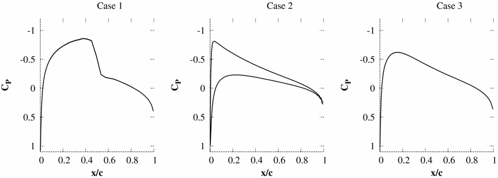
The accuracy of the pressure predicted by piston theory on the first time step directly after a pulse is tested by comparing to non-linear Euler simulations for three test cases. Only results from the first time step are considered as the instantaneous response produced by a sample pulse input at this time has been found to be the key factor in ensuring: that solutions do not encounter non-physical behaviour which prevents convergence and that the pulse is large enough to ensure a response beyond the accuracy specified for the CFD code. The test cases all use the NACA0012 aerofoil with a 25% flap, which can undergo heave and pitch (about quarter chord) motions. The mesh used has 139 × 15 cells (Fig. 1) and the flow solver is an implicit cell-centred finite volume dual-time Euler scheme based on the standard Jameson scheme. The mean flow solutions for the inviscid test cases are shown in Fig. 2.

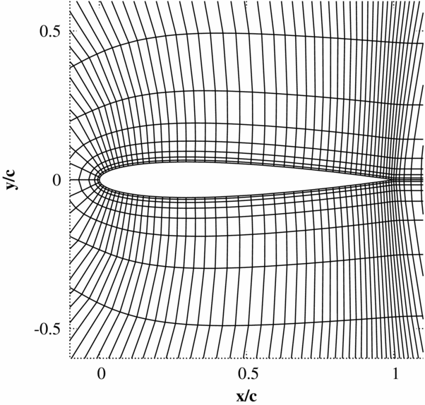
Figure 1. Finite volume Euler mesh used for all 2D Euler pulse-sizing test cases (139x15 cells, 99 cells over the aerofoil).

Figure 2. Non-linear mean flow solutions.

The velocity expansion of Equation (13) can be expressed for the pulse inputs as:

(19) $$\begin{eqnarray} \begin{array}{l@{\quad}l@{\quad}l}v_{2} & = & \left\lbrace \begin{array}{l@{\quad}l}\mathbf {V}\cdot (\mathbf {\hat{\bf n}}_{2}-\mathbf {\hat{\bf n}}_{1}) & \;\;\bar{\Delta }\alpha \; {\rm Pitch\, pulse,}\\[5pt] \left(\mathbf {a}-\mathbf {a}_{x}\right)\dot{\mathbf {\alpha }}\cdot \mathbf {\hat{\bf n}}_{2} & \;\;\bar{\Delta }\dot{\alpha }\;{\rm Pitch\, rate\, pulse},\\[5pt] 0 & \;\;\bar{\Delta }h\;{\rm Heave\, pulse},\\[5pt] \dot{\mathbf {h}}\cdot \mathbf {\hat{\bf n}}_{2} & \;\;\bar{\Delta }\dot{h}\;{\rm Heave\, rate\, pulse},\\[5pt] \mathbf {V}\cdot (\mathbf {\hat{\bf n}}_{2}-\mathbf {\hat{\bf n}}_{1}) & \;\;\bar{\Delta }\delta \;{\rm Flap\, pulse},\\[5pt] \left(\mathbf {b}-\mathbf {b}_{x}\right)\dot{\mathbf {\delta }}\cdot \mathbf {\hat{\bf n}}_{2} & \;\;\bar{\Delta }\dot{\delta }\;{\rm Flap\, rate\, pulse}\hspace{2.84526pt} \end{array} \right. \end{array} \end{eqnarray}$$

The component of normal velocity in the expansion for heave displacement is predicted to be zero as the normals do not change. The results in the following sections will show that the non-linear response to a pure heave displacement, although non-zero, remains very small.

Tables 1 and 2 give an overview of the steady flow conditions and pulse sizes used in the test cases. In Table 1, a baseline set of pulse input sizes is defined as scale = 1. These pulse size values are then scaled by a factor scale = 5 ⁿ to allow a simple rescaling of the results to check for linearity.

Table 1 Pulse Inputs

Table 2 Test Cases

The unsteady pulse responses (Figs 3–8) are shown as a change in pressure and integral force from the non-linear mean solution

(20) $$\begin{equation} \bar{\Delta }p = p_{2}-p_{1}, \end{equation}$$\\

(21) $$\begin{equation} \bar{\Delta }C_{F} = \left[C_{F}\right]_{2}-\left[C_{F}\right]_{1}, \end{equation}$$

where p is the non-dimensional static pressure and C_F is the respective integral force coefficient (F = L, M, H for lift, pitching moment and hinge moment). Again, subscripts 1 and 2 represent the values before and after the first time step when the pulse is applied. The pressure change results are shown for the four different pulse sizes (from Table 1), with the values rescaled using scale to demonstrate the approximate linearity of the response.

Figure 3. Test case 1 - Scaled pressure response $\bar{\Delta }P,$ from Equation (20) using the viscous wall condition. Responses are shown for (a) α; (b) $\dot{\alpha }$ ; (c) h; (d) $\dot{h}$ ; (e) δ; (f) $\dot{\delta }$ . The pulse magnitudes are given in Table 1.

Figure 4. Test case 1 - Integral response (C_l , C_m , C_h ). Each row corresponds to the pulse of a row in Table 1 and the points on each plot correspond to the four scales in Table 1.

Figure 5. Test case 2 - Scaled pressure response $\bar{\Delta }P,$ from Equation (20) using the viscous wall condition. Responses are shown for (a) α; (b) $\dot{\alpha }$ ; (c) h; (d) $\dot{h}$ ; (e) δ; (f) $\dot{\delta }$ . The pulse magnitudes are given in Table 1.

Figure 6. Test case 2 - Integral response (C_l , C_m , C_h ). Each row corresponds to the pulse of a row in Table 1 and the points on each plot correspond to the four scales in Table 1.

Figure 7. Test case 3 - Scaled pressure response $\bar{\Delta }P,$ from Equation (20) using the viscous wall condition. Responses are shown for (a) α; (b) $\dot{\alpha }$ ; (c) h; (d) $\dot{h}$ ; (e) δ; (f) $\dot{\delta }$ . The pulse magnitudes are given in Table 1.

Figure 8. Test case 3 - Integral response (C_l , C_m , C_h ). Each row corresponds to the pulse of a row in Table 1 and the points on each plot correspond to the four scales in Table 1.

In interpreting the results, the key measures are:

1. 1. The maximum pressure change predicted by piston theory for unit input should be of the same order of magnitude as the maximum pressure change from CFD scaled for unit pulse input. It should be noted that precise accuracy is not required as piston theory is only being used to select a pulse size.

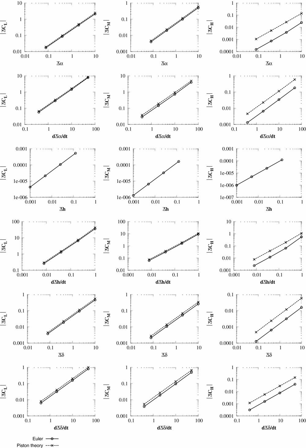
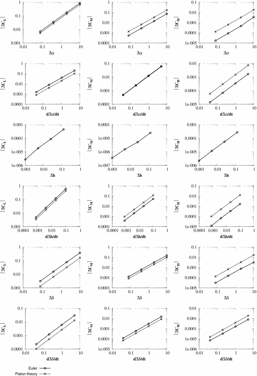
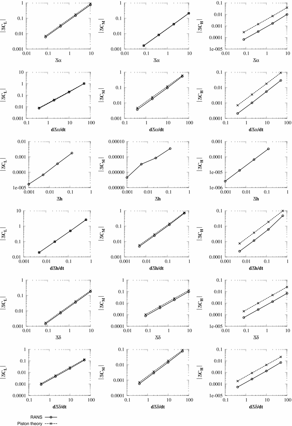
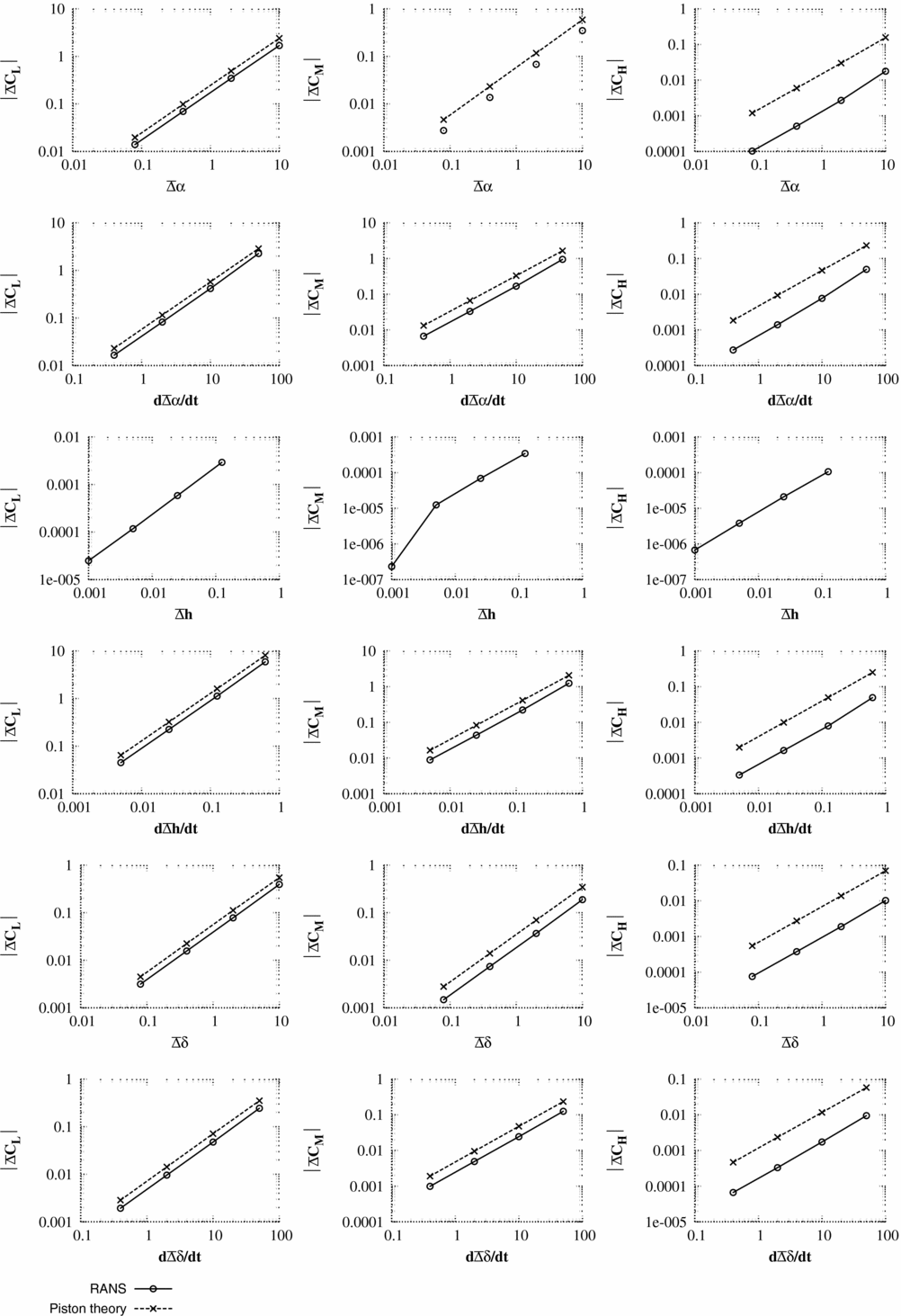
2. 2. The change in integral force coefficients predicted by piston theory should also have a similar order of magnitude to the CFD values for the same size of input. Again, precise accuracy is not required.

This is discussed further in Section 6.

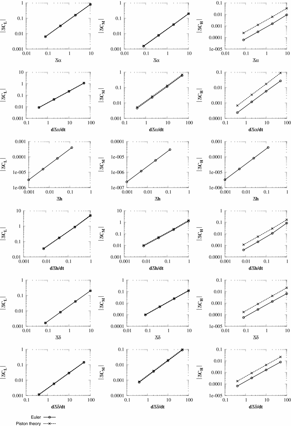
For test case 1, κ² M ² = 16 which is much greater than 1; for test case 2, κ² M ² is close to the limiting value of 1; and for test case 3, the criteria for κ² M ² is violated. For test cases 1 and 2, the initial integral values for lift and pitching moment are accurately predicted by the piston theory. As can be seen from the pressure responses, the piston theory cannot capture the merging of the trailing-edge pressure with the wake and, hence, hinge moment coefficients are less accurately predicted. Test case 3 is run at an unrealistically high time step which would not normally be encountered for aeroelastic simulations. However, even here (case 3), the correct order of magnitude of the integral forces and the maximum/minimum surface pressures is captured by piston theory. The largest pulse size (scale = 125) is selected to be unfavourably large. Many of the responses for the large pulse inputs are seen to be non-linear. For test case 3, the responses to pitch (α) and heave rate ( $\dot{h}$ ) include the influence of shock waves which were not present in the steady flow. In general, these large pulse inputs struggled with convergence and were accompanied by very large changes in the integral force values.

5.4.2 2D viscous results

As for the Euler simulations of the previous section, the pressure and the integrated forces for the first time step directly after the pulse is compared with the piston theory. The test cases used are as described for the Euler simulations with the addition that the Reynolds number for all cases is 1 × 10⁷. The mesh and steady flow solution are shown in Figs 9 and 10 for the RANS solver.

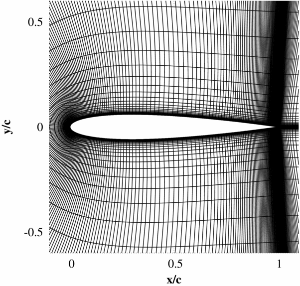
Figure 9. Finite volume Navier-Stokes mesh used for all 2D Navier-Stokes pulse sizing test cases (401x50 cells, 301 cells over the aerofoil).

Figure 10. Non-linear mean flow solutions.

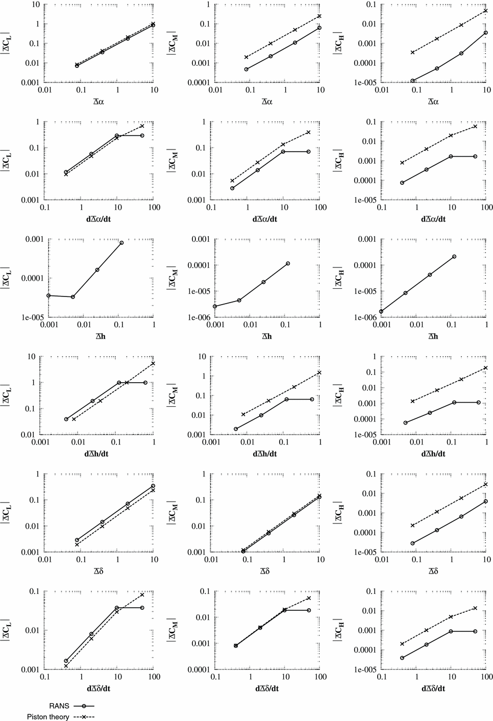
The results for the RANS/piston comparisons are shown in Figs 11–16. Unlike the Euler comparisons, where the pressure distribution was still well-predicted for Case 2, the piston theory only produces accurate pressure distributions for case 1 where Condition (18) is valid. However, the accuracy of the integrated coefficients is still excellent, even for the hinge moment if it is remembered that only an order of magnitude analysis is required.

Figure 11. Test case 1 - Scaled pressure response $\bar{\Delta }P,$ from Equation (20) using the viscous wall condition. Responses are shown for (a) α; (b) $\dot{\alpha }$ ; (c) h; (d) $\dot{h}$ ; (e) δ; (f) $\dot{\delta }$ . The pulse magnitudes are given in Table 1.

Figure 12. Test case 1 - Integral response (C_l , C_m , C_h ). Each row corresponds to the pulse of a row in Table 1 and the points on each plot correspond to the four scales in Table 1.

Figure 13. Test case 2 - Scaled pressure response $\bar{\Delta }P,$ from Equation (20) using the viscous wall condition. Responses are shown for (a) α; (b) $\dot{\alpha }$ ; (c) h; (d) $\dot{h}$ ; (e) δ; (f) $\dot{\delta }$ . The pulse magnitudes are given in Table 1.

Figure 14. Test case 2 - Integral response (C_l , C_m , C_h ). Each row corresponds to the pulse of a row in Table 1 and the points on each plot correspond to the four scales in Table 1.

Figure 15. Test case 3 - Scaled pressure response $\bar{\Delta }P,$ from Equation (20) using the viscous wall condition. Responses are shown for (a) α; (b) $\dot{\alpha }$ ; (c) h; (d) $\dot{h}$ ; (e) δ; (f) $\dot{\delta }$ . The pulse magnitudes are given in Table 1.

Figure 16. Test case 3 - Integral response (C_l , C_m , C_h ). Each row corresponds to the pulse of a row in Table 1 and the points on each plot correspond to the four scales in Table 1.

6.0 PRACTICAL APPLICATION

When running CFD codes to obtain the pulse responses needed for ERA ROM generation, piston theory is applied to size the pulses to avoid convergence issues. The following work flow process is applied:

1. 1. Generate non-linear mean flow solution

2. 2. Apply local 1D piston theory using Equation (12) to find the change in force coefficients from the mean values for a unit pulse input.

   1. (a) The required pulse size to achieve a prescribed integral force change $\triangle \overline{C}_{F}$ is achieved by scaling the linear integral force change from the piston theory. The resulting scaling factor defines the pulse input magnitude for the CFD solver.

   2. (b) Check that Equation (12) does not predict very low or negative surface pressures for the rescaled pulse size.

3. 3. Check the mesh integrity when deformed for pulse input of the size determined in step 2.

4. 4. Apply the pulse input to the CFD solver.

5. 5. Check the final response is as expected and fully captured within the accuracy of the converged solution.

It should be noted that the prescribed integral force change $\triangle \overline{C}_{F}$ depends heavily on the precision of the output and the control the user has over it. One of the main advantages of using an ERA based ROM is that little or no change to the CFD code is required; however, this means that the accuracy constraints of the output files of the code may be fixed and varies from code to code. Further, if the output forces are not the change from mean values, but absolute values, then the accuracy is also impacted by the relative ratio of the change in force coefficients to the mean force coefficient values. Thus, absolute guidelines are not possible as it will depend on the specific application.

8.0 DATA ACCESS

The data used in the figures presented in this paper are available at DOI: 10.5523/bris.mjzvu4runkof1eb3sy8sd28j8