


INTRODUCTION
The conversion of terrestrial radiocarbon (14C) ages into sidereal time requires appropriate calibration curves derived from absolutely dated archives that accurately reflect past atmospheric 14C levels. Tree rings form the gold standard if obtained from well-replicated and dendrochronologically securely dated trees (Reimer et al. Reference Reimer, Bard, Bayliss, Beck, Blackwell, Bronk Ramsey, Brown, Buck, Edwards, Friedrich, Grootes, Guilderson, Haflidason, Hajdas, Hatté, Heaton, Hogg, Hughen, Kaiser, Kromer, Manning, Reimer, Richards, Scott, Southon, Turney and van der Plicht2013a). Other archives, although forming an essential and highly valuable contribution to the current calibration curves, require various assumptions, potentially diminishing their reliability. For example, plant macrofossils contained within lake deposits (e.g. Lake Suigetsu) may experience variable residence times before incorporation into sediments, while also being susceptible to contamination because of their relatively small sample size (Bronk Ramsey et al. Reference Bronk Ramsey, Staff, Bryant, Brock, Kitagawa, van der Plicht, Schlolaut, Marshall, Brauer, Lamb and Payne2012); atmospheric 14C concentrations derived from speleothems require us to make modeling assumptions about the dead carbon fraction (Southon et al. Reference Southon, Noronha, Cheng, Edwards and Wang2012); and the accuracy of reservoir-corrected surface marine 14C dates can be compromised by variable marine reservoir ages (Reimer et al. Reference Reimer, Bard, Bayliss, Beck, Blackwell, Bronk Ramsey, Buck, Cheng, Edwards, Friedrich, Grootes, Guilderson, Haflidason, Hajdas, Hatté, Heaton, Hoffmann, Hogg, Hughen, Kaiser, Kromer, Manning, Niu, Reimer, Richards, Scott, Southon, Staff, Turney and van der Plicht2013b).
Four main factors, discussed more fully below, influence the ability of tree-ring data to provide accurate 14C calibration: differences in atmospheric 14C levels within the global atmosphere; the difference in timing of growing seasons; the accuracy, precision and reproducibility of the component 14C data sets; and finally, the fitness and rigor of the statistical model used to combine the data into a curve.
Although the precision of the calibrated age associated with a single radiocarbon determination is influenced by the accuracy and reproducibility of component data sets, it is largely dominated by the structure of the calibration curve. Crucially, the variability observed in the calibration curve arises from non-linearity in atmospheric 14C production, due to varying solar activity and geomagnetic field strength modifying impinging cosmic radiation levels, and changes in the global carbon cycle. Lengthy periods of declining 14C production, matching the rate of radiocarbon decay, result in 14C plateaux which turn precise radiocarbon measurements into extended calendar age ranges. For example, a carbon date of 2470 ± 20 BP in the center of the De Vries perturbation IIIb (Taylor and Bar-Yosef Reference Taylor and Bar-Yosef2014: Figure 2.12a) translates into a 2-sigma calendar age range spanning ∼275 yr (2715–2440 cal BP).
This inherent variability in atmospheric 14C concentration is exploited by the technique known as “wiggle-matching,” which refers to the Bayesian process of fitting several 14C determinations which have unknown absolute calendar ages, but known relative age spacing (e.g. tree rings), to a 14C calibration curve. Matching of the radiocarbon dates to the wiggles in the curve can not only significantly improve the precision of the age estimates (Galimberti et al. Reference Galimberti, Ramsey and Manning2004) but also reduces the influence of minor offsets (Bronk Ramsey et al. Reference Bronk Ramsey, van der Plicht and Weninger2001).
Many studies have benefitted from highly precise calendar ages obtained by wiggle-matching. These include the dating of critical tephra marker beds (e.g. Santorini (Manning et al. Reference Manning, Höflmayer, Moeller, Dee, Ramsey, Fleitmann, Higham, Kutschera and Wild2014), Taupo tephra (Hogg et al. Reference Hogg, Lowe, Palmer, Boswijk and Ramsey2012), locking in floating tree-ring 14C sequences for calibration purposes (e.g. Hogg et al. Reference Hogg, Southon, Turney, Palmer, Ramsey, Fenwick, Boswijk, Büntgen, Friedrich, Helle and Hughen2016) and archaeological applications (e.g. Hogg et al. Reference Hogg, Gumbley, Boswijk, Petchey, Southon, Anderson, Roa and Donaldson2017; Palmer et al. Reference Palmer, Turney, Hogg, Hilliam, Watson, van Sebille, Cowie, Jones and Petchey2014 and many others).
Radiocarbon wiggle-matching of short tree-ring series can, however, be problematic. Bayliss et al. (Reference Bayliss, Marshall, Tyers, Ramsey, Cook, Freeman and Griffiths2017) ran a series of short (25–35 ring) wiggle-matches from longer, dendrochronologically dated, Medieval period oak sequences and compared the 95% highest posterior density (HPD) credible intervals for their calibrated calendar ages against the known dendrochronological age. To correspond to their nominal coverage, one would expect approximately 95% of these credible intervals to have included the true age. However Bayliss et al. (Reference Bayliss, Marshall, Tyers, Ramsey, Cook, Freeman and Griffiths2017) found that just under half (47.7%) of the short wiggle-matches produced did not; and even 3 of the 5 long (120–207 ring) wiggle-matches were inaccurate.
Several possible reasons for such low coverage have been suggested. It may be that there are high levels of annual 14C variation which are not currently captured by the calibration curve as they are not identifiable from the blockedFootnote 1 decadal, or bidecadal, data used in its construction. Such hidden annual variations have the potential to shift a wiggle-match by a considerable margin (see e.g. Pearson et al. Reference Pearson, Brewer, Brown, Heaton, Hodgins, Jull, Lange and Salzer2018). However alternatively, and arguably more easily remedied, it may be that there are additional sources of variation present in the data—such as geographic offsets, seasonal effects, or laboratory biases—that are not suitably recognized and accounted for within the existing modeling of 14C datasets.
The recent trend of collecting large numbers of high resolution (often annual) tree-ring calibration data exposes a calibration curve to a severe risk of bias if the high-resolution measurements are made from geographically restricted areas and/or seasonally biased records. With or without decadal measurements, high resolution data have the potential to swamp other data and so it is essential that steps are taken to model the data appropriately to mitigate these risks. There is an important question that needs to be answered: how do we incorporate high resolution tree-ring 14C data into calibration curves, with the inherent risk of laboratory/geographical/seasonal bias potentially skewing the calibration curve? The current explosion of annual tree-ring accelerator mass spectrometry (AMS) analyses make this a pressing issue.
In this paper we investigate the potential presence of such additional variability (offsets/biases) in tree-ring 14C data and the effect it can have on calibration. We utilize post-Little Ice Age (LIA) AD 1500–1950 extant and new Southern Hemisphere calibration 14C data to study the sizes of such potential offsets across both location and laboratory; and introduce a new Bayesian method for curve construction, which permits each dataset to have an unknown offset from the others—potentially a laboratory, tree, or location effect. This method can adaptively estimate and incorporate possible offsets when both combining the individual calibration data into a curve and also the calibration of a new determination. Furthermore, our approach is able to identify any calibration sets which appear to have particularly large offsets in comparison to the other data. These sets can then be carefully considered and investigated further to assess their appropriateness for inclusion or otherwise. We identify one dataset which appears to have a significant offset that we discuss further for suitability for incorporating into a mid-latitude calibration curve. We compare and contrast SHCal13 compiled using a random walk model (RWM) with the curve constructed by this new approach and discuss its general suitability for international calibration. The combined impact of the new SH data sets and approach to calibration curve construction on wiggle-matching short sequences, is assessed by wiggle-matching a 14C data set derived from a 60-ring palisade post, obtained from Otāhau Pā, the first New Zealand Māori pā (fort) to be precisely dated (Hogg et al. Reference Hogg, Gumbley, Boswijk, Petchey, Southon, Anderson, Roa and Donaldson2017). We also assess the impact of variable atmospheric radiocarbon levels on wiggle-matching short tree-ring sequences in the post-LIA interval by conducting a large number of simulations using the Bayesian calibration program OxCal (Bronk Ramsey et al. Reference Bronk Ramsey, van der Plicht and Weninger2001; Bronk Ramsey Reference Bronk Ramsey2009).
FACTORS INFLUENCING CALIBRATION ACCURACY
Currently only two atmospheric 14C reservoirs are recognized for pre-AD 1950 material, with terrestrial samples calibrated using either Northern Hemisphere (NH, IntCal) or Southern Hemisphere (SH, SHCal) calibration curves. The ability of an atmospheric calibration curve to supply accurate calendar age information for dates derived from samples from a specific locality is influenced by four factors:
1. Differences in atmospheric 14C levels within each of the two reservoirs (intra-hemispheric homogeneity), which may vary with time;
2. The difference in timing of growing seasons;
3. The accuracy, precision and reproducibility of component data sets; and
4. The suitability of the statistical approach that combines the component 14C data sets into the calibration curve, and the linked approach used to calibrate a new determination against it.
Intra-Hemispheric and Inter-Hemispheric Offsets
An inter-hemispheric North/South (N/S) 14C offset (e.g. 44 ± 17 yr for the time interval 195 BC to AD 1845; Hogg et al. Reference Hogg, Palmer, Boswijk and Turney2011), probably resulting from a higher sea-air 14CO2 flux from the larger expanse of SH oceans (Rodgers et al. Reference Rodgers, Mikaloff-Fletcher, Bianchi, Beaulieu, Galbraith, Gnanadesikan, Hogg, Iudicone, Lintner, Naegler and Reimer2011), is now well established (Hogg et al. Reference Hogg, Hua, Blackwell, Niu, Buck, Guilderson, Heaton, Palmer, Reimer, Reimer and Turney2013a). Braziunas et al. (Reference Braziunas, Fung and Stuiver1995) developed a three-dimensional global circulation model (GCM), which described atmospheric 14C contours in response to oceanic boundary conditions. The model predicted a decline of atmospheric Δ14C of 1‰ (~8 14C yr) per 10° of latitude, to a maximum of 5‰ between 50°N and 50°S. Although intra-hemispheric (regional) offsets have been claimed in numerous studies (e.g. in Japan, Nakamura et al. Reference Nakamura, Masuda, Miyake, Nagaya and Yoshimitsu2013 and Korea, Hong et al. Reference Hong, Park, Park, Sung, Park and Lee2013), unambiguous evidence for these offsets has remained elusive. Most importantly of all, a lack of quasi-simultaneous analysis of contemporaneous local/calibration curve sample pairs has hindered distinguishing regional from laboratory analytic offsets. To address this issue, McCormac et al. (Reference McCormac, Baillie, Pilcher and Kalin1995) analyzed 9 sample pairs of dendrochronologically secure bristlecone pine and Irish oak for the interval 500–320 BC and found a mean offset of –41 ± 9.2 14C yr. Of the three suggested reasons for the offset (regional differences, wood pretreatment and dendrochronological issues), the authors concluded that published data reveal evidence for small location dependant (and possibly time varying) differences, which may be important for high precision wiggle-matching. Intensities of the high energy AD 775 14C spike have recently been measured in tree rings from Japan, California, Siberia, Poland, Germany, and New Zealand (Park et al. Reference Park, Southon, Fahrni, Creasman and Mewaldt2017). All NH measurements show statistically similar intensities, with the New Zealand data ∼6‰ lower (Park et al. Reference Park, Southon, Fahrni, Creasman and Mewaldt2017), consistent with the measured N/S offset. It should be noted that strictly speaking, IntCal and SHCal are mid-latitude curves (Reimer et al. Reference Reimer, Bard, Bayliss, Beck, Blackwell, Bronk Ramsey, Buck, Cheng, Edwards, Friedrich, Grootes, Guilderson, Haflidason, Hajdas, Hatté, Heaton, Hoffmann, Hogg, Hughen, Kaiser, Kromer, Manning, Niu, Reimer, Richards, Scott, Southon, Staff, Turney and van der Plicht2013b; Hogg et al. Reference Hogg, Hua, Blackwell, Niu, Buck, Guilderson, Heaton, Palmer, Reimer, Reimer and Turney2013a).
The Difference in Timing of Growing Seasons
It is postulated that regional offsets could be linked to differences in the timing of growing seasons for plants, possibly as a result of variations in the seasonal flux of 14CO2 from the stratosphere into the troposphere (Kromer et al. Reference Kromer, Manning, Kuniholm, Newton, Spurk and Levin2001; Manning et al. Reference Manning, Kromer, Kuniholm and Newton2001, Reference Manning, Höflmayer, Moeller, Dee, Ramsey, Fleitmann, Higham, Kutschera and Wild2014). Although this mechanism is often cited for small (e.g. ∼20 yr) offsets from IntCal, many of the studies (e.g. Dee et al. Reference Dee, Brock, Harris, Ramsey, Shortland, Higham and Rowland2010; Manning et al. Reference Manning, Höflmayer, Moeller, Dee, Ramsey, Fleitmann, Higham, Kutschera and Wild2014) have not directly dated paired regional/IntCal samples. There is therefore always the possibility of analytic offsets, either connected with the analysing laboratory or with the datasets composing IntCal. The ideal way of establishing small regional offsets is by quasi-simultaneous counting (for radiometric labs) or measurement within the same wheel (for AMS labs). Unfortunately, this is rarely done and the question about the existence of measurable seasonal 14C gradients is still open to debate.
The Accuracy, Precision and Reproducibility of Component Data Sets
Calibration curves utilize a compilation of data generated by different laboratories at different times and using different analytic approaches. Although international intercomparisons suggest that radiocarbon laboratories are generally accurate and precise (e.g. Scott et al. Reference Scott, Naysmith and Cook2017), more rigorous intercomparisons analyzing successive tree rings have shown that laboratory analytic offsets can exist (e.g. Hogg et al. Reference Hogg, Turney, Palmer, Southon, Kromer, Ramsey, Boswijk, Fenwick, Noronha, Staff and Friedrich2013b). Accurate calibration is also dependent upon accurate, precise and reproducible component data sets. Three factors influencing the development of accurate and precise calibration datasets are dendrochronological reliability, efficiency of pretreatment processes to remove contaminating modern or background contamination, and the measurement method. Tree-ring series with weak dendrochronological linkages can result in serious calibration curve errors. For example, the beginning of the “absolute tree-ring chronology” (Friedrich et al. Reference Friedrich, Remmele, Kromer, Hofmann, Spurk, Kaiser, Orcel and Küppers2004) was revised from 12,410 cal BP to 12,325 cal BP (Hogg et al. Reference Hogg, Turney, Palmer, Southon, Kromer, Ramsey, Boswijk, Fenwick, Noronha, Staff and Friedrich2013b; M. Friedrich, IntCal dendro-meeting in Zürich, August 2015) leaving significant errors in IntCal13 (Hogg et al. Reference Hogg, Southon, Turney, Palmer, Ramsey, Fenwick, Boswijk, Büntgen, Friedrich, Helle and Hughen2016). Wood pretreatment procedures can vary significantly and range from more rapid acid-base-acid (ABA) processes to intensive alpha-cellulose extraction. Pretreatment effectiveness is influenced by sample age, preservation environment, species and sample size and what is effective in one study may not be suitable for another. It is important the labs undertaking 14C measurements for calibration purposes initially determine appropriate pretreatment methods (see Southon and Magana Reference Southon and Magana2010; Capano et al. Reference Capano, Miramont, Guibal, Kromer, Tuna, Fagault and Bard2018 for examples). Furthermore, tree-ring 14C measurements can be made by both AMS and radiometric methods, with both having their strengths and weaknesses. While AMS has considerable potential for high resolution single ring dating and is likely to revolutionize tree-ring radiocarbon calibration, the mg-sized samples are more susceptible to modern contamination, compared with high precision radiometric samples which are of the order of 1500 times larger.
Statistical Approaches for Curve Construction
The current calibration curves, IntCal13 and SHCal13, use a random walk model (RWM) approach (Niu et al. Reference Niu, Heaton, Blackwell and Buck2013) which was also used for IntCal09 and Marine09 (Blackwell and Buck Reference Blackwell and Buck2008; Heaton et al. Reference Heaton, Blackwell and Buck2009). This approach considered the change in the radiocarbon age from one year to the next to vary according to a normal distribution (a random walk). For the tree-ring-based portion of the curve, it was assumed that there were no possible additional sources of uncertainty beyond that reported by the laboratory. All the tree-ring observations were thus modeled as:
 $${X_i} = {\rm{}}\mu \left( {{\theta _i}} \right) + {\rm{}}{\epsilon_i},$$
where X i is the observed radiocarbon age of a tree ring of known calendar age θi; μ(θ) is the underlying calibration curve at calendar age θi; and  ${\epsilon_i}\sim N\left( {0,\sigma _i^2} \right)$ the reported lab uncertainty.
This approach does not permit the possibility that any offsets (laboratory, geographical, genera, etc.) may exist between groups of data. However, it can be seen that there appear to be time periods (e.g. AD 1800–1950) where the raw data are more dispersed than such a model would suggest. Furthermore, the consequence of this model is that, as more data become available, even if they are more scattered or offset, the credible intervals of the estimated calibration curve will narrow and potentially lead to overly precise and inaccurate calibration of new determinations. This would likely further exacerbate the low credible interval coverage seen in Bayliss et al.’s (Reference Bayliss, Marshall, Tyers, Ramsey, Cook, Freeman and Griffiths2017) wiggle-match study.
The above issues could be addressed within the RWM but the International Calibration Working Group (IntCal) has decided to no longer use this approach in future IntCal and SHCal upgrades. The RWM was extremely slow to run which both removed the opportunity to investigate the effect of model assumptions or individual datasets; and made it difficult to assess convergence of the Markov Chain Monte Carlo (MCMC) used to fit the model. Instead, the new IntCal curves will utilize a Bayesian Spline approach which is computationally more efficient while still maintaining the required rigor and ability to incorporate the unique features of the calibration datasets from different sources (both tree and non-tree based).
We present this new approach in summary only here; and only for the known age tree-ring-based data. A full statistical explanation of the new Bayesian Spline methodology and its application to data with uncertain calendar ages will be given elsewhere (Heaton et al. Reference Heaton, Blaauw, Blackwell, Ramsey, Reimer and Scott2019). However we do describe how potential offsets between data can be incorporated in curve construction.
NEW CURVE CONSTRUCTION METHODOLOGY
Basic Bayesian Splines
Rather than modeling evolution of the radiocarbon age over time, the planned Bayesian spline approach considers Δ14C directly. Specifically, we model the atmospheric value of Δ14C at time θ as,
 $${{\rm{\Delta }}^{14}}C\left( \theta \right) = {\rm{}}\mathop \sum \limits_{i = 1}^K {\beta _i}{B_i}\left( \theta \right)$$
where Bi (⋅) are B-spline basis functions at a pre-chosen, fixed set of knots and β = (β 1,…, β K)T are the unknown basis coefficients that determine the curve. Curve construction then proceeds by trying to choose a balance between a curve that goes close to the observed determinations but is also not overly rough which would likely be overfitting the data.
We achieve this by first specifying a prior that penalizes over-variation in the level of Δ14C over time,
 $$\pi (\beta {\rm{|}}\lambda ) \propto \exp \left( { - \gamma {\rm{ }}\int {{{\left\{ {{\Delta ^{14}}C''\left( \theta \right)} \right\}}^2}} d\theta } \right).$$
Here γ is a smoothing parameter that defines the trade-off between fidelity to the data; and variation in the level of atmospheric radiocarbon. By modeling the curve in Δ14C this penalty on roughness is constructed in a domain where, before observing data, we might believe the curve would exhibit approximately similar roughness over its history. This prior has the effect that we will not introduce spurious wiggles to our estimated calibration curve where they are not supported by the data itself.
The posterior for the Δ14C curve is then found by finding a compromise between this prior and goodness-of-fit to the observed calibration data. Due to the blocking and the uncertainties in the calendar ages of the older (>14kyr) objects used to construct IntCal, it is easiest to assess this goodness-of-fit in the F 14C domain. For a determination that represents a block of ni years, we model the observed corrected fraction modern Fi for each object as
 $${F_i} = {\rm{}}{1 \over {{n_i}}}\mathop \sum \limits_{j = 0}^{{n_i} - 1} {F^{14}}C\left( {{\theta _i} + j} \right) + {\rm{}}{\epsilon_i},$$
where F 14C(θ) is the transformation of the calibration Δ14C curve at time θ and  ${\epsilon_i}\sim N\left( {0,\sigma _i^2} \right)$ is the reported lab uncertainty. This rigorous and exact incorporation of blocking in the data was not done for IntCal13 and SHCal13.
We assess fidelity in the F 14C domain, as opposed to the radiocarbon age scale used for the IntCal13 and ShCal13 methodologies, since observational uncertainties are symmetric in F 14C. Again this offers an advance on IntCal13 and SHCal13 since, in the radiocarbon age domain, as we progress further back in time, the uncertainties on the observed radiocarbon ages can become significantly asymmetric. See Heaton et al. (Reference Heaton, Blaauw, Blackwell, Ramsey, Reimer and Scott2019) for more details.
Including Offset Terms
To include the potential for offsets in the radiocarbon age shared by a particular data set we adjust our model so that Xi, the observed radiocarbon age of a tree-ring datum i, is considered as
 $${X_i} = {1 \over {{n_i}}}\mathop \sum \limits_{j = 0}^{{n_i} - 1} {\mu} \left( {{\theta _i} + j} \right) + {\rm{}}{\zeta _{j\left( i \right)}} + {\eta _i}$$
with ζ j(i) the potential offset shared by all observations in the set j. This can be incorporated into our Bayesian Spline approach via adjusting our assessment of fidelity in the F 14C domain to
 $${F_i} = {\gamma _{j\left( i \right)}}{\rm{}}\left\{ {{1 \over {{n_i}}}\mathop \sum \limits_{j = 0}^{{n_i} - 1} {F^{14}}C\left( {{\theta _i} + j} \right)} \right\} + {\rm{}}{\epsilon_i},$$
with γ j(i) = eζj(i)/8033 the F 14C domain multiplier that equates to an offset ζ j(i) in the radiocarbon age.
We place a prior on the size of potential offset ζ j(i)∼N(0, τ 2). For this study, we use a relatively uninformative prior by setting τ = 20. In fitting the model we are provided with not only posterior estimates of the calibration curve (through the spline coefficients β ) but also the estimated offsets ζ j(i) for each dataset.
Model Estimation
Estimation of both the curve and the offsets is performed via MCMC. Unlike the RWM which required updating the value of the calibration curve one year at a time, the Bayesian spline model described above can be estimated using Gibbs sampling where the entire curve is updated simultaneously along its entire history. This makes estimation and convergence much quicker. Note that in estimation we also place uninformative priors on the smoothing parameter λ and update this within the sampler (see Heaton et al. Reference Heaton, Blaauw, Blackwell, Ramsey, Reimer and Scott2019 for further details).
Impact on Calibration and Wiggle-Matching
The inclusion of potential offsets in our modeling also has an impact upon calibration of either a new, unknown age, radiocarbon determination or a wiggle-match. If one considers there may be potential offsets in the datasets that make up the calibration curve, then one should also include the possibility that a new, undated determination may also be offset. In the case of a single determination, this is equivalent to using the prediction interval of the calibration curve (rather than the credible interval). In the case of a wiggle-match, it is equivalent to introducing a potential shift up/down to the undated object before judging the quality of curve fit. In OxCal terms this would be considered a Delta_R adjustment. For our illustrative wiggle-match of the Otāhau Pā palisade post we include such an adjustment using both the OxCal Delta_R with a uniform prior ζ j(i)∼U[−20, 20]; and the same prior for offset as in curve construction i.e. ζ j(i)∼N(0, τ 2) with τ = 20.
APPLICATION OF NEW METHODOLOGY
Example 1: Recreating SHCal13
To assess the new curve construction methodology and to evaluate SHCal13 data component offsets, we first built a new version of the calibration curve using the same five datasets as SHCal13 (see Table 1). Figure 1 shows individual data points together with the 1 sigma SHCal13 curve (SHCal13-RWM) and the new curve (SHCal-NEW).
Table 1 Summary of SHCal13 AD 1500–1950 tree-ring chronologies and data sets showing segment lengths (# rings) and number of analyses (N). QL: Quaternary Isotope Lab; Wk: Waikato University; UB: Queens University Belfast; PTA: Pretoria; OZ: ANSTO. GPC: gas proportional counting; HPLSC: high precision liquid scintillation counting; AMS: accelerator mass spectrometry.
* Data sets 2 and 3 obtained from splits of the same wood samples.
+ “solv. extr.” = solvent extracted.

Figure 1 SHCal13 data sets 1–5, AD 1650–1950. Legend = Lab identifier, source of wood. SHCal13-RWM = SHCal13 curve as published, using the random walk model; SHCal13-NEW = new curve compiled using Bayesian splines with offsets, from SHCal13 data only. The Wk measurements from AD 1725-1935 are not shown as they were inadvertently left out of SHCal04 and SHCal13. The PTA AD 1850 value of 129 ± 14 yr BP as shown here and as given in the SHCal04 and SHCal13 data sets (http://intcal.qub.ac.uk/shcal13/query/) is incorrect: the value should be 155 ± 11 yr BP (corrected in Figure 3).
SHCal13-NEW follows predominantly the same shape as SHCal13-RWM although it appears in some time periods (e.g. AD 1760–1800 and 1900–1920) that the SHCal13-NEW estimates shows higher inter-annual variation, as indicated by more highly attenuated peaks and troughs.
In the periods where the curve drops between AD 1680–1710 and 1800–1820, the SHCal-RWM mean estimate lies somewhat below the SHCal13-NEW mean estimate (although still within the 1-sigma SHCal13-NEW envelope). Here we are mainly dependent upon QL data to inform the value of the curve—any potential offset in this data will therefore introduce a bias to the curve unless we incorporate it in modeling. In regions where QL data overlaps with other data, QL lies consistently younger in comparison suggesting such a bias may exist. Unlike the RWM, the Bayesian Splines Offset approach allows the possibility of such a QL laboratory offset and permits the entire QL set to shift upwards to provide a better overall fit. Since the QL data are the largest data set throughout the period of study, the overall mean of SHCal-NEW is slightly older than SHCal-RWM. Between AD 1650–1820, the mean of SHCal-NEW is on average 6.3 yr older. Between AD 1825–1900 the mean new curve averages 1.3 yr older.
The credible intervals for the curve created using Bayesian splines (with potential offsets) are wider than that created with the RWM. The 1-sigma intervals for SHCal13-NEW predominantly contain the 1-sigma intervals for SHCal13-RWM. The Bayesian spline method generates a curve with an average uncertainty σ of 13.9 over this time period, compared with the RWM of 10.7. This is likely due to the additional uncertainty caused by the incorporation of potential offsets. The wider envelope on the SHCal13-NEW curve means that when calibrating a radiocarbon determination against it, the credible range for the object’s unknown age will generally be wider than the interval obtained by calibrating against SHCal13-RWM, the latter we consider unrealistically precise.
The relative offsets estimated by the new curve compilation method range from –7.1 to +4.5 yr, see Table 2, with the QL and UB data sets negative and the Wk, PTA and OZ offsets positive. The total range between the posterior means of the offsets is 11.6 yr and the standard deviation is 5.6. Of particular interest are that data sets ID 2 and 3 (and 6 in Table 3 below) contain measurements made by the Wk and UB laboratories on splits of the same wood samples. These measurements are on trees from the same location and species, providing some indication of the potential sizes of offsets between laboratories. The posterior mean difference between the Wk and UB data sets for these common wood samples is 12.8 ± 3.9 yr (with Wk older).
Table 2 Relative offset data for SHCal13 tree rings from AD 1500–1950 by different laboratories (refer to Table 1). Offsets calculated by the SHCal13-NEW curve compilation method.

Table 3 Summary of new AD 1500–1950 SH tree-ring chronologies/data sets showing segment lengths (# rings) and number of analyses (N). HPLSC: high precision liquid scintillation counting; AMS: accelerator mass spectrometry.

* Wk* = samples analyzed at Waikato University for C. Turney.
^ 1915-1945 decades given preliminary multiple solvent (acetone) extractions.
¶ duplicate analyses.
# 1931–1950 decades from Takapari FP (40°04’S, 175°59’E).
+ “solv. extr.” = solvent (acetone) extracted.
‡ kauri derived from the upper North Island of New Zealand but exact geographic location unknown.
Example 2: Inclusion of New Data and Outlier Identification
Our next illustration demonstrates the inclusion of six other SH data sets compiled since the release of SHCal13. Here we aim to highlight both how this influences the width of the curve’s credible interval, and how the offsets estimated by the method can be used to flag potential outlying datasets for further investigation.
Table 3 provides details of the tree-ring chronologies and 14C data sets. To be suitable for calibration purposes, tree-ring 14C data sets must be derived from a dendrochronologically securely dated piece of wood with appropriate wood pretreatment methods (Reimer et al. Reference Reimer, Bard, Bayliss, Beck, Blackwell, Bronk Ramsey, Brown, Buck, Edwards, Friedrich, Grootes, Guilderson, Haflidason, Hajdas, Hatté, Heaton, Hogg, Hughen, Kaiser, Kromer, Manning, Reimer, Richards, Scott, Southon, Turney and van der Plicht2013a).
Dendrochronology
Set 6: Wk-Hihitahi (dendrochronology—L. Xiong, J. Palmer).
The New Zealand cedar (Libocedrus bidwillii) chronology network is well established and has been used for palaeoclimate reconstructions (Xiong and Palmer Reference Xiong and Palmer2000a, Reference Xiong and Palmer2000b; Palmer and Xiong Reference Palmer and Xiong2004). The Hihitahi site is part of the network and consists of 49 crossdated trees spanning AD 1431–1991 with all the ring-width measurements lodged in the International Tree-ring Data Bank (ITRDB; newz066.rwlFootnote 2). The specific tree selected for this study (H4702) was one of several dead trees found at the site and crossdated over the period AD 1456–1960 (505 yr). A site tree-ring chronology was compiled in the program COFECHA (Holmes Reference Holmes1983) from all the individual measurement series (after first being standardised to a mean of zero and standard deviation of 1.0). The selected tree had a Pearson correlation of 0.462 to the site chronology (once the series being tested had been removed from the master chronology; Grissino-Mayer Reference Grissino-Mayer2001).
Set 7: Wk*-Hihitahi (dendrochronology—L. Xiong, J. Palmer).
The same tree (H4702) as previously used from Hihitahi (Set 6, above) was re-sampled for the time period AD 1701–1930. However, even though only a relatively small amount of wood was needed for the AMS dating there was insufficient remaining for the last two decadal samples (i.e. 1931–1950) (Turney et al. Reference Turney, Palmer, Hogg, Fogwill, Jones, Bronk Ramsey, Fenwick, Grierson, Wilmshurst, O’Donnell and Thomas2016). To complete the program we chose to use samples from a tree (TKP144) at another adjacent site (Takapari; ITRDB listing newz062.rwl). The Takapari site chronology covers AD 1256–1992 and the selected tree spans AD 1704–1989 with a Pearson correlation of 0.485 to the Takapari site master chronology.
Set 8: Wk*-Doughboy (dendrochronology—J. Palmer).
The pink pine (Halocarpus biformis) chronology from this site was originally developed by D’Arrigo et al. (Reference D’Arrigo, Buckley, Cook and Wagner1996) and updated in Palmer et al. (Reference Palmer, Cook, Turney, Allen, Fenwick, Cook, O’Donnell, Lough, Grierson and Baker2015). The site chronology of 65 trees covers AD 1457–2010 (all measurements lodged on the ITRDB; newz118.rwl). The samples taken for radiocarbon dating were from a dead fallen tree (DBY225) that crossdated over the period AD 1620–1965 (346 yr) with a Pearson correlation of 0.597 to the master dating chronology (Turney et al. Reference Turney, Palmer, Hogg, Fogwill, Jones, Bronk Ramsey, Fenwick, Grierson, Wilmshurst, O’Donnell and Thomas2016).
Set 9: Wk*-Lake Tay (dendrochronology—J. Palmer).
The pioneering development of a chronology from Callitris columellaris from Lake Tay in southern Western Australia (Cullen and Grierson Reference Cullen and Grierson2009) was recently updated with additional cores and cross-sections. This data is yet to be publicly available as more samples are currently being processed. Two different trees were used for the radiocarbon sample series—LTY14-37 for the period AD 1701–1800 and LTY14-05 for AD 1801–1950 (Turney et al. Reference Turney, Palmer, Hogg, Fogwill, Jones, Bronk Ramsey, Fenwick, Grierson, Wilmshurst, O’Donnell and Thomas2016). The first tree (LTY14-37) crossdated for 311 yr at AD 1630–1940 (Pearson correlation to the master series of 0.444) while the second tree (LTY14-05) crossdated for the shorter time period of AD 1790–2010 (221 yr) with a Pearson correlation of 0.557.
Set 10: Wk*-Campbell Island (dendrochronology—J. Palmer).
A 140-year chronology was produced from the small tree/shrub species Dracophyllum longifolium from the remote subantarctic Campbell Island (Turney et al. Reference Turney, Fogwill, Palmer, van Sebille, Thomas, McGlone, Richardson, Wilmshurst, Fenwick, Zunz, Goosse, Wilson, Carter, Lipson, Jones, Harsch, Clark, Marzinelli, Rogers, Rainsley, Ciasto, Waterman, Thomas and Visbeck2017; ITRDB listing newz117.rwl). The radiocarbon samples were taken from tree CMB05 that crossdated from AD 1900–2012 (Turney et al. Reference Turney, Palmer, Hogg, Fogwill, Jones, Bronk Ramsey, Fenwick, Grierson, Wilmshurst, O’Donnell and Thomas2016) and had a Pearson correlation to the master series of 0.392.
Set 11: Wk-Auckland (dendrochronology—G. Boswijk).
The kauri (Agathis australis) timber SPC002 (AD 1590–1849) used for dataset 11 was derived from one of seven cross-sectional slices obtained from large kauri beams that had been incorporated into the sub-floor structure of a 1930s transitional bungalow located on the grounds of St Pauls College, Richmond Road, Ponsonby, Auckland. All series were compared against each other using the crossdating program CROS73 (Baillie and Pilcher Reference Baillie and Pilcher1973) included in Dendro for Windows (Tyers Reference Tyers1997). All matches were checked using visual alignment of line graphs. SPC002 crossmatched with five timbers, with intra-site Baillie-Pilcher t-values (BPt) values ranging from 3.12 to 7.96 (mean T = 5.46; standard deviation [s.d.] = 1.80). SPC002 was calendar dated against a kauri master, and crosschecked against independent modern and archaeological chronologies (T values ranging from 3.36 to 9.58 [N = 14; mean T = 6.70; s.d. = 1.66]).
Pretreatment
Because tree-ring 14C data has been collected from different species, it is important to pretreat the samples to a reliable wood fraction that reflects ambient atmospheric conditions at time of growth and is not affected by species-specific differences or variable lignin contents.
Pretreatment schemes for each data set are summarised in Table 3. Details for the solvent-extracted alpha-cellulose pretreatment for HPLSC are given in Hoper et al. (Reference Hoper, McCormac, Hogg, Higham and Head1998). In summary, wood is ground to pass a 20-mesh sieve, refluxed in Soxhlet apparatus using ethanol-chloroform, bleached with acidified NaClO2 followed by a base/acid extraction. The AMS alpha-cellulose pretreatment (Turney et al. Reference Turney, Palmer, Hogg, Fogwill, Jones, Bronk Ramsey, Fenwick, Grierson, Wilmshurst, O’Donnell and Thomas2016) involves ABA/bleaching with acidified NaClO2/ABA. Solvent extracted alpha-cellulose for AMS utilizes preliminary multiple acetone extractions to remove resins followed by the alpha-cellulose pretreatment described for AMS samples above.
Pretreatment Issues Connected with Resinous Wood Species
Despite many pretreatment studies finding resin removal by solvent extraction unnecessary (e.g. Vogel et al. Reference Vogel, Fuls, Visser and Becker1986: 935, “it has been repeatedly shown that this organically soluble matter cannot influence the results noticeably”), and ABA pretreatment as effective as cellulose extraction (e.g. Capano et al. Reference Capano, Miramont, Guibal, Kromer, Tuna, Fagault and Bard2018), it is important that all tree species being utilized for calibration purposes be tested to demonstrate this. Two of the species (Halocarpus biformis and Callitris columellaris) utilized by Turney et al. (Reference Turney, Palmer, Hogg, Fogwill, Jones, Bronk Ramsey, Fenwick, Grierson, Wilmshurst, O’Donnell and Thomas2016) are very resinous and inadequate removal of resins in samples close to the nuclear weapons testing 14C boundary in age would have led to analytic errors if an initial solvent extraction preceding alpha-cellulose preparation was not utilized. Figure 2 shows 14C ages with and without preliminary solvent extractions.

Figure 2 Doughboy Bay (Halocarpus biformis) and Lake Tay (Callitris columellaris) duplicate analyses with and without solvent pretreatment prior to alpha-cellulose extraction. Elevated 14C levels due to nuclear weapons testing, peaking in the SH in 1965 (Turney et al. Reference Turney, Palmer, Maslin, Hogg, Fogwill, Southon, Fenwick, Helle, Wilmshurst, McGlone and Ramsey2018), have been translocated by resins across earlier rings and only removed by a preliminary solvent extraction. Non-solvent extracted Wk*-Hihitahi analyses (Libocedrus bidwillii) are given for comparison.
An Initial Fit with RWM and Bayesian Splines
Individual data points are plotted in Figure 3 together with the 1 sigma SHCal13 curve (SHCal13-RWM) and the new curve (SH-All-NEW). Table 4 provides details of the relative offsets between the various data sets. We see that the majority of the new datasets have offsets that are of similar size to the offsets in the five sets used for SHCal13—with offsets in the region of –8 to 6 yr. However we clearly also identify an outlying dataset from Campbell Island with an estimated posterior mean offset of 22 ± 9 yr worthy of more detailed investigation. First however we briefly discuss each dataset in turn.
Table 4 Relative offsets of all available SH tree-ring 14C data sets (AD 1500–1950).


Figure 3 SHCal13 data sets 1–5, with new data sets, 6–11, AD 1650–1950. Legend = lab identifier, source of wood. Wk* = samples analyzed at Waikato University for C. Turney. SHCal13-RWM = SHCal13 curve as published; SHCal-All-NEW = new curve compiled from all 11 potential SH data sets. The correct PTA AD 1850 value of 155 ± 11yr BP is shown here.
Data Set 6: Libocedrus bidwillii from Hihitahi, NZ.
Decadal measurements from NZ cedar sourced from Hihitahi State Forest Park were made by Waikato University using HPLSC and published in McCormac et al. (Reference McCormac, Hogg, Higham, Lynch Stieglitz, Broecker, Baillie, Palmer, Xiong, Pilcher, Brown and Hoper1998). This data set was inadvertently overlooked in the SHCal04 and SHCal13 iterations. The wood fraction dated was solvent extracted alpha-cellulose (see Hoper et al. Reference Hoper, McCormac, Hogg, Higham and Head1998). The Wk-Hihitahi L. bidwillii data set has a mean offset of +5.7 ± 6.8 yr, which is broadly similar to the offset of Wk measurements in SHCal13 (+3.3 ± 8.8 yr—Table 2).
Data Sets 7, 8, 9, 10.
Decadal measurements from Hihitahi Forest Park (set 7), Doughboy Bay, Stewart Island, NZ (set 8), Lake Tay, Western Australia (set 9) and Campbell Island, NZ (set 10) were made by the Waikato AMS laboratory and published in Turney et al. (Reference Turney, Palmer, Hogg, Fogwill, Jones, Bronk Ramsey, Fenwick, Grierson, Wilmshurst, O’Donnell and Thomas2016). The alpha-cellulose wood fraction was dated with details of the pretreatment methods given in Turney et al. (Reference Turney, Palmer, Hogg, Fogwill, Jones, Bronk Ramsey, Fenwick, Grierson, Wilmshurst, O’Donnell and Thomas2016). The youngest samples (i.e., AD 1940–1950) from the resin-rich Doughboy and Lake Tay sites were subject to an initial solvent extraction to remove mobile components (resins, etc.) translocating 14C generated by atomic weapons testing across the ring boundaries.
The AMS data sets from Hihitahi, Doughboy Bay and Lake Tay broadly follow SHCal13 with mean offsets of –6.2 ± 6.6 yr, –0.8 ± 6.8 yr and 3.7 ± 6.7 yr respectively.
Although the Lake Tay offset of 3.7 ± 6.7 yr shows these data generally conform to the average of the other data sets, some of the measurements suggest the possibility of pre-AD 1950 resin translocation across ring boundaries. The decades centered on AD 1825 and 1875 for example, appear to be unusually offset from the mean SH-ALL-NEW curve. We re-analyzed these 2 data points with initial solvent extractions (Figure 4) and although the new results are not statistically different from the initial analyses, both solvent-extracted data points are more conformable. For the purposes of this paper, we have retained the Lake Tay data but further investigations into Lake Tay Callitris columellaris will be required before these data can be accepted for 14C calibration purposes. The Campbell Island measurements have an offset of 22.2 ± 9.0 yr and are discussed in more detail below.
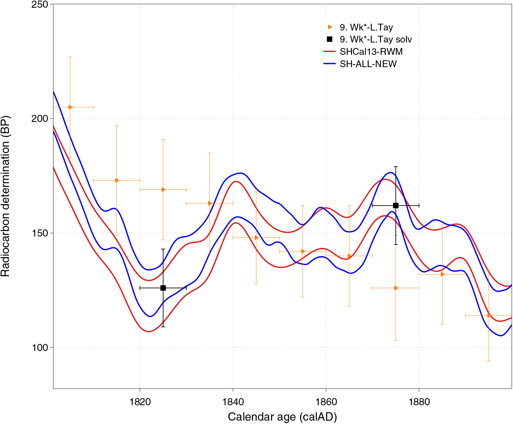
Figure 4 Lake Tay (Western Australia) AD 1825 and 1875 tree-ring 14C analyses with and without solvent pretreatment prior to alpha-cellulose extraction. The solvent extracted values conform more closely to the SH-ALL-NEW curve suggesting the possibility of resin translocation across ring boundaries.
Data Set 11: Agathis australis from Auckland, NZ.
Replicate 5-ring segments of kauri were analyzed by the Waikato AMS laboratory for the interval AD 1650–1829. The data, previously shown in graphic form only in Hogg et al. (Reference Hogg, Gumbley, Boswijk, Petchey, Southon, Anderson, Roa and Donaldson2017) are given in Table 5. All duplicated analyses are statistically consistent at the 5% significance levels (Ward and Wilson Reference Ward and Wilson1978). The data follow the shape of SHCal13 closely and have an offset to the mean of all 11 data sets of 1.7 ± 5.8 yr.
Table 5 Agathis australis tree-ring 14C data—sample SPC002 (AD 1650–1829).

The SH calibration curve SHCal13 (Figure 1) contains three higher resolution QL South American Nothofagus data points centered on AD 1819.5 (3-ring), 1824 (2-ring), 1828 (5-ring). If the QL analyses had a systematic (perhaps temporal) offset towards younger ages, the high resolution data would have the potential to overly influence the calibration curve towards younger ages at this time. Because of the potential impact of this upon wiggle-matching short tree-ring sequences, we extended the 5-year kauri measurements to overlap with this period (Figure 5). The new kauri data centered on AD 1817, 1822, and 1827 are considerably older than the equivalent QL data, and are more comparable with measurements from the other data sets. The apparent QL offset appears to be analytic in nature. Unpublished South American Fitzroya decadal data (De Pol-Holtz pers. comm. 2018) centered on decades AD 1818.5 and 1828.5 are also older (Figure 5) suggesting a geographic offset at this time is unlikely.

Figure 5 SH-REFINED-NEW calibration curve constructed from accepted data sets 1–9 and 11. SHCal13 curve given for comparison. The two decadal South American Fitzroya data points centered on AD 1818.5 and 1828.5 are courtesy of Dr Ricardo De Pol-Holz and have not been used in curve construction.
Outlying Campbell Island—A Geographic Offset?
The estimated Campbell Island offset of 22.2 ± 9.0 yr clearly sets this dataset apart from the rest. However it is important not to simply discard data because they appear to be outlying but instead investigate the potential reasons behind such occurrences. Outliers may be genuine erroneous measurements in which case they should be removed; but alternatively they may represent genuine phenomena, in which case they should not only be kept but one should also think about what the implications of such real phenomena might be.
In our case, the Campbell Island, Hihitahi, Doughboy Bay, and Lake Tay samples were pretreated and graphitized as a group in the Waikato AMS laboratory, with the graphite samples measured in the same AMS wheel at the UCI Keck AMS laboratory. A large offset from any one of these 4 data sets is therefore unlikely to be analytic and more likely to be geographic in nature. As Campbell Island lies at 52°S amidst the Southern Ocean, the high 14C ages (low 14C concentration) probably result from dilution by outgassed old CO2 associated with Southern Ocean upwelling (Turney et al. Reference Turney, Palmer, Hogg, Fogwill, Jones, Bronk Ramsey, Fenwick, Grierson, Wilmshurst, O’Donnell and Thomas2016). The ability to identify data sets with geographic biases is an important and innovative characteristic of this new method of curve construction.
In light of this, since we are aiming to provide a mid-latitude SHCal curve, we choose to discard Campbell Island from the calibration data. It should however provide a key note of caution for those wishing to calibrate data arising from locations adjacent to the Southern Ocean.
Construction of a New Southern Hemisphere Calibration Curve for the Interval AD 1500–1950
The new Bayesian Spline curve fitting regime described above has identified 10 suitable from 11 possible datasets for construction of a new SH calibration curve (SH-REFINED-NEW) for the interval AD 1500–1950, with the omission of data set 10 (Campbell Island) for the reasons given above. After a refitting of the Bayesian spline on these 10 datasets, the resultant calibration curve can be seen in Figure 5 with the relative offsets given in Table 6. The same figure (Figure 5) also shows the SHCal13-RWM published output using just the five datasets available in 2013.
Table 6 Relative offsets of the 10 suitable SH tree-ring 14C data sets (AD 1500–1950), combined to produce curve SH-REFINED-NEW.

Many of the features discussed in Example 1 (Recreating SHCal13) can again be seen when comparing the Bayesian spline SH-REFINED-NEW estimate (using the selected 10 datasets) against the SHCal13-RWM estimate (using just the five datasets). The Bayesian spline model and the addition of the new data sets do not change the overall shape of the curve significantly although peaks and troughs in the curve are more attenuated with SH-REFINED-NEW. The mean of SH-REFINED-NEW is still somewhat lower where the curve drops between AD 1680–1710 and 1800–1820, as a result of the curve in these regions being highly influenced by the QL data which, when compared to the rest of the data in this time period, seems to be consistently younger, suggesting a possible offset.
Importantly, despite the addition of the five new data sets, the width of the 1-sigma interval of SH-REFINED-NEW is still larger than the SHCal13-RWM estimate based on only five data sets. The average uncertainty σ for SH-REFINED-NEW is 12.2 over this time period, compared with the average SHCal13-RWM σ of 10.7. This suggests that offsets between datasets really are present in calibration data. As described earlier, there is evidence that the existing RWM can provide estimates that are overly precise which in turn leads to inaccurate calibration. Therefore a method that does not provide estimates with higher precision than the RWM, even after the inclusion of additional data which one might expect to increase precision, is probably desirable.
The total offset range for the refined curve is 14.9 yr, with a standard deviation of 5.5. These values are comparable with those values found for SHCal13 (SHCal13 range = 11.7 yr; s.d. = 5.6). Based on these findings, we suggest that new datasets with offsets lying significantly outside these ranges (such as the Campbell Island data) be examined carefully but should not however be automatically excluded.
RADIOCARBON WIGGLE-MATCHING
Part of the motivation for determining the component offsets of suitable SH data sets was to investigate the accuracy of radiocarbon wiggle-matching in the AD 1500–1950 time range. We were primarily interested in two aspects of wiggle-matching short sequences: (1) the accuracy and precision of wiggle-matching using the new SH curve SH-REFINED-NEW compared with SHCal13; (2) using OxCal and SH-REFINED-NEW in a process of simulation to estimate the level of precision likely to be achieved when wiggle-matching short sequences, from archaeological material for example.
The inclusion of offsets in curve construction has consequences for calibration. If there are potential offsets in the datasets used to create the calibration curve, similar offsets should be considered to exist in any data set that we might calibrate—especially since the data going into the calibration curve is considered particularly high quality. We therefore need to incorporate such a potential offset for our undated sample when performing our calibration procedure. This will typically have the effect of widening the intervals of calibrated dates.
Comparison of SHCal13 and the New Curve SH-REFINED-NEW for Wiggle-Matching Short Sequences
To compare the effect of both the new curve methodology, and the incorporation of potential offsets, for wiggle-matching sequences with short segment lengths, we utilized a 60-ring (12 five-ring segments) Prumnopitys ferruginea (miro) palisade post 14C data set obtained from Otāhau Pā, Taupiri, New Zealand (Hogg et al. Reference Hogg, Gumbley, Boswijk, Petchey, Southon, Anderson, Roa and Donaldson2017). We investigate both the effect on the wiggle-match when using the SHCal13 curve and SH-REFINED-NEW curve; and also when one does, or does not, recognize the possibility that the undated sample may also have an offset.
Inclusion of offsets in datasets during calibration can be done in OxCal via the Delta_R function (Bronk Ramsey Reference Bronk Ramsey2009). OxCal however does not have the feature to incorporate the blocking present in the radiocarbon determinations of our palisade post, i.e. that each section of the post relates to the average of a 5-year segment and not just a single year. It also does not currently allow use of an annually resolved calibration curve (instead taking a subsampled output on a coarser 5-year grid). We therefore also include our own wiggle-match procedure that both permits us to use our annually resolved SH_REFINED_NEW curve fully; and also recognizes and includes the blocking in the palisade post when determining the wiggle-match.
We performed five comparison wiggle-matches:
Using SHCal13
i. OxCal with no incorporation of a possible offset in palisade post and no recognition of palisade blocking;
ii. OxCal with a potential palisade post offset modeled as Delta_R but no recognition of palisade blocking;
Using SH-Refined-New
iii. OxCal with no incorporation of a possible offset in palisade post and no recognition of palisade blocking;
iv. OxCal with potential post offset modeled as Delta_R but no recognition of palisade blocking;
v. Personally coded approach using annually resolved calibration with both recognition of palisade blocking and potential post offset.
When using OxCal and including a potential miro palisade post offset, we applied the OxCal Reservoir Offset (“Delta_R”) with a uniform prior of −20 to +20 yr (i.e. Delta_R(““,U(−20,20)). All OxCal wiggle-matches also employed outlier analysis (Bronk Ramsey Reference Bronk Ramsey2009) using Outlier_Model (“SSimple”,N(0,2),0,”s”) with {Outlier, 0.05} (which allows individual samples—roughly 1 in 20—to be outliers) to down-weight outliers. For wiggle match v) that incorporated fully the 5-year blocking within the wiggle-match, we modeled the potential offset term as ζ∼N(0, 202) to mirror SH-REFINED-NEW’s curve construction.
We report the estimated calendar age of the most recent (outermost) tree ring in the Miro post in Table 7 and graph the post’s determinations against the two curves in Figure 6.
Table 7 Summary of wiggle-matching New Zealand Prumnopitys ferruginea (miro) post 005 14C data against SHCal13 and SH-REFINED-NEW. Age estimates correspond to the most recent (outermost) tree ring in the post.

(† and *) These wiggle-matches included a potential offset ζ between the miro post and the calibration curve datasets. The OxCal wiggle-matches (†) utilize a uniform Delta_R prior Delta_R(“Wk”,U(−20,20)); the exact blocking (*) modeled the offset as ζ∼N(0, 202) to match the curve construction. The code used for the exact blocking approach did not estimate ζ directly since it is not required to perform calibration.

Figure 6 Unknown calendar-age 14C results from the New Zealand Prumnopitys ferruginea (miro) palisade post 005 plotted against SHCal13 and SH-REFINED-NEW calibration curves.
We note that this period of the calibration curve has a reverse and rapidly changing slope in the ~AD 1715–1750 interval (Figure 6). Because of this, and contrary to what is normally expected, the oldest 14C miro post dates are associated with felling of the tree (outside rings—highest ring numbers), and the younger 14C dates associated with the time of initial growth (center rings—lowest ring numbers).
It is likely this unique aspect of the miro post is the reason that little difference is seen between the calibrated age ranges for the different methods. Considering the effect of including offsets on your undated sample when calibrating, for the miro post the wiggle-match can only fit well at one individual time period whether or not it is believed to be offset. However, the inclusion of possible offsets in data to be calibrated does have a much larger effect in general, and especially on single sample observations, where it serves to widen the credible intervals. Regarding the difference between the two curves, we do see some minor differences in the calibrated age ranges between the SHCal13 and SH-REFINED-NEW curves, with the SH-REFINED-NEW placing the tree slightly older albeit only by a few years.
Simulation of Probable Levels of Precision When Wiggle-Matching Short Sequences in the Interval AD 1500–1950
We used OxCal and our Bayesian spline annual curve (SH-REFINED-NEW) in a process of simulation to estimate the level of precision likely to be achieved when wiggle-matching short tree-ring sequences (as typically found in palisade posts) in the interval AD 1500–1950 (Figure 7). We undertook 10 simulations with end points every decade through this period. The coloured squares represent the average total 95% calibrated age range span (oldest cal BP date minus youngest cal BP date)—lower is better. The vertical axis “Number” shows how the 95% range span changes by increasing the number of radiocarbon determinations per wiggle-match, from a minimum of one (a single determination covering the entire 60-rings) to a maximum of 12 (i.e. 12 determinations of 5-ring blocks in a 60-ring palisade post). Using the example of the miro post wiggle-match discussed above, the Bayesian spline approach with SH-REFINED-NEW produced a range end date of AD 1766 and a total range span of 9 yr (Table 7). Figure 7 shows that a high level of precision such as this can be achieved with as few as five determinations per wiggle-match for time ranges with sufficient structure in the calibration curve (e.g. AD 1670–1700; AD 1760–1820). The simulations also show that 60-ring sequences may not be long enough to produce precise wiggle-matches for some time intervals, due to repeating structures (for example, AD 1620–1640, AD 1860–1890).

Figure 7 Average total 95% calibrated age range (oldest cal BP date minus youngest cal BP date) when wiggle-matching 60-ring segment lengths during the interval AD 1500–1950. Simulations using SH-REFINED-NEW calibration curve with segment length of 60 yr (rings). Precision (1σ error) = ± 15 14C yr. Large number of simulations often give multiple solutions, resulting in a high average range. Where there are repeating structures that could be confused, the average ranges are longer.
There is clear structure from the calibration curve SH-REFINED-NEW in Figure 7. For the New Zealand Otāhau Pā palisade post example the outermost youngest rings lie in a zone of highest available precision (dark blue 95% probability range span of <10 yr. The time period before AD 1650 is more problematic with a large 14C plateaux influencing the interval ∼AD 1450–1650 and resulting in probable ranges of 20–30 yr or more, even with a 60-ring wiggle-match containing 12 determinations. The very low precision (high ranges) associated with calendar ages younger than AD 1850 may be less of a concern if historical records for this later period can be used as a terminus post quem.
CONCLUSIONS
The precision associated with 14C wiggle-matching of tree rings is impacted by the non-monotonic form of the 14C calibration curve, the accuracy and precision of component data sets, and the statistical approach to producing the curve. This paper sought to investigate these factors through the presentation of a new Bayesian spline method for curve construction which was then tested on extant and six new SH data sets (also examining their dendrochronological reliability and pretreatment) for the post-LIA interval AD 1500–1950. The new method of construction allows calculation of component data offsets, permitting identification of laboratory and geographic biases. This enabled us to identify two features of independent interest.
Firstly, we observe the presence of a potential geographical offset at subantarctic Campbell Island. Data from this site shows high offset values probably due to its high latitude in the Southern Ocean and hence we suggest it should be excluded from future SHCal updates. Secondly, measurement of splits of the same wood samples in both Wk and UB laboratories provided information on the potential sizes of analytical offsets between laboratories. Our study suggested such laboratory offsets may lie in the region of 12.8 ± 3.9 yr. This implies that high-resolution data sets need to be compiled by at least two different laboratories to mitigate the impact of individual laboratory biases distorting the calibration curves.
In addition to the above, we investigated the effect of pre-treatment methods. The Western Australia Lake Tay data compiled from highly resinous Callitris columellaris trees shows some data points which may be influenced by resin translocation across ring boundaries. Further work is required to determine the suitability of these measurements for calibration purposes.
Application of the new calibration method to the 10 suitable SH 14C data sets suggests that individual offset ranges for component data sets, appear to be in the region of ±10 yr. Data sets with individual offsets larger than this need to be carefully assessed before selection for calibration purposes. A wiggle-match of 12 five-year segments from a New Zealand miro palisade post produced similar results using the new method of curve construction (and new data) when compared with OxCal using SHCal13. This is likely due to the unique shape of the post’s 14C determinations lying on an inversion of the calibration curve. In general, we expect that the new method of curve construction will provide somewhat wider credible intervals when calibrating objects against it, a desirable feature given recent evidence for possible over-precise and inaccurate wiggle-matching using current calibration curves (Bayliss et al. Reference Bayliss, Marshall, Tyers, Ramsey, Cook, Freeman and Griffiths2017).
Importantly, simulations using OxCal and the new SH curve suggest that wiggle-matching short sequences (e.g. less than ~60-rings) can however produce accurate wiggle-matches that still have high levels of precision (e.g. ranges of less than ∼10 yr) in the AD 1650–1850 interval. Earlier and later time periods in the time interval AD 1500–1950 containing 14C plateaux or repeating structures may produce lower levels of precision, with ranges of 20–30 yr or more.


