


1. Introduction
The addition of a small amount of a polymer or surfactant to a Newtonian fluid reduces the frictional drag of the flow and delays the transition to turbulent flow. Drag reduction phenomena have been extensively studied for many decades to elucidate their fundamental principles and design fluid transportation systems to realize energy saving (Virk et al. Reference Virk, Merrill, Mickley, Smith and Mollo-Christensen1967; Pinho & Whitelaw Reference Pinho and Whitelaw1990; Zakin, Myska & Chara Reference Zakin, Myska and Chara1996; Escudier, Nickson & Poole Reference Escudier, Nickson and Poole2009; Zakin & Ge Reference Zakin and Ge2010). An important feature of these phenomena is the anisotropic effect, i.e. as wall-normal velocity fluctuations decrease, streamwise velocity fluctuations increase (Den Toonder, Nieuwstadt & Kuiken Reference Den Toonder, Nieuwstadt and Kuiken1995; Den Toonder et al. Reference Den Toonder, Hulsen, Kuiken and Nieuwstadt1997). This feature, which is observed in polymer solutions, is attributable to polymer extension in the flow of the solutions (Lumley Reference Lumley1973; Wei & Willmarth Reference Wei and Willmarth1992; Den Toonder et al. Reference Den Toonder, Nieuwstadt and Kuiken1995, Reference Den Toonder, Hulsen, Kuiken and Nieuwstadt1997; Graham Reference Graham2014). The extension of polymers caused by the polymer coil–stretch transition in turbulent flow influences the turbulent energy transfer in the flow. Min et al. (Reference Min, Yoo, Choi and Joseph2003) suggested that the kinetic energy in the near-wall region is transported as the elastic energy stored in the extended polymers to the buffer and the log layer.
The relaxation time of the polymers should be sufficiently long for effective energy transfer. Therefore, the polymer extension estimated by the Weissenberg number and the relaxation time becomes an important parameter. The relaxation time of the polymers should be comparable to the characteristic time scale of the flow to achieve drag reduction (Owolabi, Dennis & Poole Reference Owolabi, Dennis and Poole2017). Polymer extension and relaxation in the flow of polymer solutions induce structural changes in the turbulent flow in the near-wall region (Li et al. Reference Li, Kawaguchi, Yu, Wei and Hishida2008; Fu et al. Reference Fu, Otsuki, Motozawa, Kurosawa, Yu and Kawaguchi2014; Motozawa et al. Reference Motozawa, Sawada, Ishitsuka, Iwamoto, Ando, Senda and Kawaguchi2014; Tamano, Kitao & Morinishi Reference Tamano, Kitao and Morinishi2014). Xi and Graham, and following related works, numerically revealed very weak streamwise vortices and elongated and smooth low-speed streaks near the wall region for the channel flow of a polymer solution (Xi & Graham Reference Xi and Graham2010; Graham Reference Graham2014; Whalley et al. Reference Whalley, Dennis, Graham and Poole2019). Furthermore, the instantaneous degrees of polymer stretching and drag reduction have been found to be temporally anticorrelated (Tamano, Graham & Morinishi Reference Tamano, Graham and Morinishi2011). The polymers stretch in active turbulence and induce a subsequent hibernation period, i.e. a weak turbulent flow. During the hibernation period, the drag is low and the polymers relax (Kushwaha, Park & Graham Reference Kushwaha, Park and Graham2017; Wang, Shekar & Graham Reference Wang, Shekar and Graham2017; Zhu et al. Reference Zhu, Schrobsdorff, Schneider and Xi2018, Reference Zhu, Bai, Krushelnycky and Xi2019).
In addition to polymers, wormlike micellar surfactant solutions induce drag reduction. Although polymer degradation in a pipe decreases the drag reduction efficiency of polymer solutions, as wormlike micelles can reassemble, they can maintain their drag reduction ability. Thus, wormlike micellar surfactant solutions are used in many circular systems such as air-conditioning systems and heat exchangers (Aguilar, Gasljevic & Matthys Reference Aguilar, Gasljevic and Matthys2001; Li, Kawaguchi & Hishida Reference Li, Kawaguchi and Hishhida2004, Reference Li, Kawaguchi and Hishida2005a; Gasljevic, Aguilar & Matthys Reference Gasljevic, Aguilar and Matthys2007; Wei et al. Reference Wei, Kawaguchi, Li, Yu, Zakin, Hart and Zhang2009; Shi et al. Reference Shi, Wang, Fang, Talmon, Ge, Raghavan and Zakin2011; Poole Reference Poole2020; Soares Reference Soares2020). The heat transfer ability of a wormlike micellar surfactant solution is often examined together with the drag reduction ability of the solution (Hara, Maxson & Kawaguchi Reference Hara, Maxson and Kawaguchi2019). Vortex deformation at the near-wall region in the flow of surfactant solutions has been intensively studied previously (Li et al. Reference Li, Kawaguchi, Sagawa and Hishida2005b, Reference Li, Kawaguchi, Yu, Wei and Hishida2008; Tamano et al. Reference Tamano, Kitao and Morinishi2014, Reference Tamano, Uchikawa, Ito and Morinishi2018; Fu et al. Reference Fu, Iwaki, Motozawa, Tsukahara and Kawaguchi2015; Hara, Tsukahara & Kawaguchi Reference Hara, Tsukahara and Kawaguchi2020). Li et al. (Reference Li, Kawaguchi, Yu, Wei and Hishida2008) visualized the vortex structure based on instantaneous velocity fields and showed that the growth angle of vortex packets below a hairpin vortex was decreased in the flow of surfactant solutions. The drag-reducing surfactant solution inhibits the process of ejection and sweep, therefore reducing the Reynolds stresses (Li et al. Reference Li, Kawaguchi and Hishhida2004, Reference Li, Kawaguchi and Hishida2005a,Reference Li, Kawaguchi, Sagawa and Hishidab; Wei et al. Reference Wei, Kawaguchi, Li, Yu, Zakin, Hart and Zhang2009).
Some features of surfactant drag reduction were found to be similar to those of polymer solutions. However, surfactant solutions also exhibit unique phenomena (Zakin & Ge Reference Zakin and Ge2010). First, wormlike micelles are easily broken and reassembled in the flow that occurs in surfactant solutions. The formation of micelles is affected by the surfactant concentrations and concentrations of counter-ion suppliers, such as sodium salicylate. The viscoelasticity of the solution is also affected by these concentrations and does not vary linearly. Because of these nonlinear phenomena and the properties of wormlike micellar solutions, several relaxation times of surfactant solutions have been observed (Lu et al. Reference Lu, Zheng, Davis, Scriven, Talmon and Zakin1998). Suzuki et al. (Reference Suzuki, Higuchi, Watanabe, Komoda, Ozawa, Nishimura and Takenaka2012) showed that wormlike micellar solutions may have single, double and triple relaxation times depending on the concentration of surfactants and counter ions. A solution containing a relatively low concentration of surfactant and counter ions is viscoelastic and has a triple relaxation time.
A solution containing a relatively high concentration of surfactant and counter ions is less viscoelastic and has a single relaxation time. These fluid properties affect turbulence characteristics, such as temporal fluctuations of the local velocities and drag reduction abilities (Suzuki et al. Reference Suzuki, Nguyen, Nakayama and Usui2005). Furthermore, the formation of high-order wormlike micellar structures is also influenced by shear stress at the wall; such structures are called shear-induced structures (SISs) (Ohlendorf, Interthal & Hoffmann Reference Ohlendorf, Interthal and Hoffmann1986; Clausen et al. Reference Clausen, Vinson, Minter, Davis, Talmon and Miller1992). Although the SIS has been investigated in many previous studies, the relationship between the structure and turbulence statistics has not been elucidated (Li et al. Reference Li, Kawaguchi, Sagawa and Hishida2005b). This is because visualization of the SIS in the flow of surfactant solutions is difficult. In addition, the formation of a well-developed structure requires a very long channel entry length. The so-called stress deficit may arise from the short entry length, which hinders the development of the flow and SIS (Suzuki et al. Reference Suzuki, Fuller, Nakayama and Usui2004). These characteristic features of surfactant solutions, such as breakup and reassembly, the presence of several relaxation times, and formation of the SIS, may result in complex interactions between wormlike micelles and turbulence.
We have been studying the effects of extensional rheological properties of polymer solutions on drag reduction using a self-standing flowing soap film to achieve a quasi-two-dimensional (2-D) flow (Hidema et al. Reference Hidema, Suzuki, Hisamatsu, Komoda and Furukawa2013, Reference Hidema, Suzuki, Hisamatsu and Komoda2014, Reference Hidema, Suzuki, Murao, Hisamatsu and Komoda2016, Reference Hidema, Murao, Komoda and Suzuki2018, Reference Hidema, Fukushima, Yoshida and Suzuki2020). Two-dimensional turbulent flow is easily formed on flowing soap films by inserting a comb of equally spaced cylinders into the flow (Rutgers et al. Reference Rutgers, Wu, Bhagavatula, Petersen and Goldburg1996; Rivera, Vorobieff & Ecke Reference Rivera, Vorobieff and Ecke1998; Boffetta & Ecke Reference Boffetta and Ecke2012). Two-dimensional turbulent flow is relatively free from shear stress, and continuous extensional stress can be applied to the flow. In the case of a conventional turbulent pipe flow, only the average shear stress caused by the mean flow is applied to the flow. Extensional flow also occurs between vortices in a pipe flow, and this induces polymer extension and an increase in extensional viscosity, which contributes to drag reduction. However, in pipe flow, extensional flow is limited in both time and space. Conversely, in the case of 2-D turbulent flow, a continuous extensional flow occurs in the region between the two cylinders and behind each cylinder in the flow. A wide area around the cylinders is affected by the extensional rate. Shear flow also occurs at the cylinder surface and behind each cylinder; however, the area is highly limited at the surface and the impact of continuous extensional rates behind the cylinder is relatively large compared with the pipe flow. Thus, vortex shedding at the cylinder is mainly affected by continuous extensional flow. Therefore, compared with pipe flow, 2-D flow and 2-D turbulent flow formed downstream as a result of the merging of vortices have advantages in observing the effects of the extensional rheology of the solution on turbulent flow. Thus, findings obtained in 2-D turbulent flow in terms of the extensional rheology help understanding the effects of extensional flow occurring in three-dimensional (3-D) turbulent flow (Graham Reference Graham2014).
In our previous study, we found that a polymer-doped solution deformed the vortices shed at the comb and the deformation was influenced by the relaxation time of the solution measured using a capillary breakup extensional rheometer (CaBER, Thermo Scientific) (McKinley & Tripathi Reference Mckinley and Tripathi2000; Anna & McKinley Reference Anna and Mckinley2001; Rodd et al. Reference Rodd, Scott, Cooper-White and Mckinley2005). The vortex deformation induced modification of the 2-D turbulent flow and a characteristic peak of the turbulent energy, k (m2 s−2), appeared without the production, P (m2 s−3), of the turbulent energy. The advantage of 2-D turbulent flow is that we can easily calculate turbulence statistics such as k, P, diffusion D (m2 s−3) and dissipation ε (m2 s−3) of the turbulent energy. The calculation of these turbulence statistics in 3-D flows requires simultaneous measurement to obtain the three-direction instantaneous velocity components, which is very difficult to achieve. Therefore, many experimental studies have measured the vortex deformation of drag-reducing flows in the 2-D plane of a 3-D flow, assuming that the average statistic value is constant in time and space. However, drag-reducing flows are often non-uniform, both temporally and spatially (Xi & Graham Reference Xi and Graham2010; Graham Reference Graham2014; Kushwaha et al. Reference Kushwaha, Park and Graham2017; Wang et al. Reference Wang, Shekar and Graham2017; Zhu et al. Reference Zhu, Schrobsdorff, Schneider and Xi2018, Reference Zhu, Bai, Krushelnycky and Xi2019; Whalley et al. Reference Whalley, Dennis, Graham and Poole2019).
In this study, we focus on the effects of the extensional rheological properties of a drag-reducing surfactant solution on the vortex deformation and turbulence statistics of 2-D turbulent flow. The vortex shedding and velocity fields behind the comb were visualized using interference patterns of the illumination light and particle image velocimetry (PIV). As mentioned above, wormlike micelles are more complex than polymers. The viscoelasticity of a wormlike micellar solution is affected by the concentration of surfactants and counter-ions. Furthermore, SIS or any other structure can form in the flow and as the structure is broken and reassembled, which may cause several relaxation times. We aim to discuss how the complex structures of wormlike micelles affect turbulent flow and to verify the similarities and differences between wormlike micellar solutions and polymer solutions.
2. Experimental procedures
2.1. Materials and measurement of rheological properties
Oleylbishydroxyethylmethyl ammonium chloride (trade name: Lipothoquad O/12, Lion Specialty Chemicals Co, Ltd.) as a cationic surfactant was dissolved in ultrapure water at a concentration of 4000 ppm. To form wormlike micelles, sodium salicylate was added to the surfactant solution as a counter-ion supplier. The molar ratio of sodium salicylate, ξ (−), to the surfactants was adjusted from 0.35 to 0.5. The drag reduction ability of the solution at room temperature was verified using the drag coefficients measured by conventional pressure drop experiments (Hidema et al. Reference Hidema, Suzuki, Hisamatsu, Komoda and Furukawa2013).
The shear viscosity, η (Pa s), of each sample solution was measured using a rheometer (MCR301, Anton Paar) with a cone-plate device at shear rates from 10 to 1000 s−1. The diameter of the cone plate device was 50 mm. When ξ was higher than 0.45, η developed with time and the time to obtain stable η increased. Thus, η was measured at a constant shear rate,  $\dot{\gamma }$ (s−1), for a sufficiently long time to obtain a stable value and the stable η at each
  $\dot{\gamma }$ combined in the range of 10 to 1000 s−1.
The extensional properties of the sample solutions were evaluated based on the relaxation time. The relaxation time of the sample solutions under extensional stress was measured using the optically detected elastocapillary self-thinning dripping-onto-substrate (ODES-DOS) technique proposed by Dinic et al. (Reference Dinic, Zhang, Jimenez and Sharma2015). The ODES-DOS system visualizes and analyses the capillary-driven thinning and pinch-off dynamics of the columnar neck in an asymmetric liquid bridge created by dripping the sample solution onto the substrate. ODES-DOS can detect the relaxation time of a very dilute solution that is not in the measurable range of commercially available shear and extensional rheometers, including CaBER. As shown in figure 3(a), a contact angle meter (Dropmaster DMs-401, Kyowa Interface Science) was used as a light source and to control the syringe that dripped the sample solution onto a surface. The gauge of the syringe needle was 12G, i.e. the inner diameter was 2.16 mm. For visualization and recording, a high-speed video camera (Fastcam Mini AX100, Photoron) with a lens (AI Micro-Nikkor 105 mm f/2.8S, Nikon) and an additional super macro lens was used. The frame rate of the high-speed video camera was set to 12 500 f.p.s. The thinning process of the liquid column, Dliquid (mm), was obtained by image analysis using Image J and Delphi (Embarcadero Technologies). Dliquid was plotted as a function of time t (s), which was fitted using the fitting function Dliquid = Aexp(−t/3λ) to calculate the relaxation time. Here, A (m) is a constant determined experimentally.
In the present study, the pinch-off process of surfactant solutions measured by ODES-DOS was similar to that of Newtonian fluids, especially in the solution with ξ ≤ 0.4. However, the formation of high-order wormlike micellar structures was enhanced under continuous shear or extensional stresses, which may occur in 2-D flow, as described in § 2.2. Thus, we evaluated the spinnability of the sample solution after continuous shear. The sample solution was installed in a rheometer (MCR301: Anton Paar) and a continuous shear rate of 100 s−1 was applied to a parallel-plate for several minutes. Subsequently, the shear was suspended and the plate was lifted to evaluate the spinnability, which was recorded using a video camera (Fastcam Mini AX100, Photoron).
2.2. Experimental apparatus used to create flowing soap films and visualize the flows
The experiments were performed using the apparatus shown in figure 1(a). A complete image of the flowing soap film as a 2-D flow is shown in figure 1(b). The details of the apparatus are provided elsewhere (Hidema et al. Reference Hidema, Murao, Komoda and Suzuki2018, Reference Hidema, Fukushima, Yoshida and Suzuki2020). The flow was driven by gravity; thus, the velocity achieved a constant value of approximately 300 mm behind the injection nozzle (Rutgers et al. Reference Rutgers, Wu, Bhagavatula, Petersen and Goldburg1996). The streamwise mean velocity, Um (m s−1), that is, the time- and special-averaged velocity, was calculated by the local velocities measured by the PIV. The period of time to calculate Um was approximately 5 s; the area to calculate Um was 35 × 25 mm2 just below the comb. The Um was approximately 1.2–1.6 m s−1 when the flow rate, Q (l s−1), was fixed at 25 ml min−1. The mean thickness of the water layer, h (m), was approximately 3.5–4.7 μm.
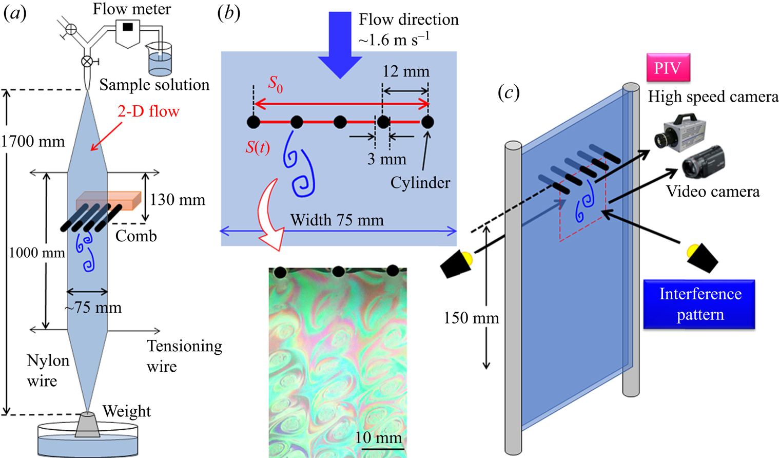
Figure 1. Schematic of the experimental apparatus. (a) Entire apparatus. (b) Cross-section deformed by the comb, which affects the local extensional rate and vortex shedding. (c) Two appropriate positions for the illumination lights for PIV and interference pattern observations.
To achieve a 2-D turbulent flow on the flowing soap films, a comb composed of equally spaced cylinders was inserted perpendicular to the flow at a position 130 mm downstream of the beginning of the parallel section in the channel. The diameter of the cylinder, d (m), was 3 mm and the spacing of the cylinder was fixed at 12 mm, as shown in figure 1(b). The Reynolds number, Re (−), was calculated using Um, the viscosity of each sample solution, the diameter of the cylinder and the water density; Re was approximately 4600. As shown in figure 2, the viscosities of solutions with ξ ≥ 0.45 increased at a certain shear stress. In this case, the viscosity measured at lower shear rates was used as the solution viscosity to calculate Re in the flow. When the comb was inserted into the flow, the sudden decrease and increase in the cross-sectional area of the water layer at the comb induced a local velocity distribution. The distribution induced shear and extensional flows around each cylinder. The shear rate calculated by the local velocity measured by PIV reached a maximum value of approximately 1000 s−1 at the obliquely downward position of each cylinder. However, the area of high shear rates was limited to less than 1 mm from the cylinder surface. In the case of the extensional rates, based on the calculation of the local velocity fluctuation measured by PIV, a higher extensional rate over 1000 s−1 was observed in a larger area, such as the area between two cylinders and the region behind the cylinder. Thus, the flow that produced vortices in the 2-D flow was stretched by the high extensional stress around the cylinder (François et al. Reference François, Lasne, Amarouchene, Lounis and Kellay2008; Asano, Watanabe & Noguchi Reference Asano, Watanabe and Noguchi2018). In addition, the time required to orient the wormlike micelles by extensional stress was shorter than that by shear stress. Therefore, the extensional stress has a greater impact on the flow passing through the comb than the shear stress around the cylinder.

Figure 2. Shear viscosity of each surfactant solution.
The mean value of the extensional rate,  $\dot{\varepsilon }$ (s−1), was estimated as
  $S(t) = S_0\exp (-\dot{\varepsilon }t)$ based on the cross-sectional area of the water layer before deformation, S 0 (m2), the cross-sectional area after deformation, S(t) (m2), and time, t (s), required for the deformation from S 0 to S(t). The value of
  $\dot{\varepsilon }$ was approximately 290 s−1 under the experimental conditions used in this study (figure 1b) (Hidema et al. Reference Hidema, Murao, Komoda and Suzuki2018, Reference Hidema, Fukushima, Yoshida and Suzuki2020). As briefly described above, to obtain more precise information about the velocity fields, the local velocity gradient around the cylinder arising from the local velocity distribution was calculated on the basis of the velocity field obtained by PIV, which is a substitute for local extensional rates (figure 9). The local extensional rate based on the PIV measurements reached more than 1000 s−1, which is much larger than the mean value
  $\dot{\varepsilon } = 290\;{\rm s}^{{-}1}$. In the case of the region behind the cylinder, continuous extensional stress as well as continuous shear stress were observed. The increase in the continuous local extensional and shear stress between the cylinders and behind the cylinder promotes the formation of high-order wormlike micellar structures in the surfactant solution; this affects the vortex shedding at the comb and, thus, the 2-D turbulent flow, as described in §§ 3.2–3.4.
The flow was visualized using the interference pattern and PIV in the region indicated in figure 1(c). The interference patterns reveal information about the thickness of the water layer in the 2-D flow. The vortices observed through the interference patterns in the observation area correspond to the vorticity of the flow (Rivera et al. Reference Rivera, Vorobieff and Ecke1998; Hidema et al. Reference Hidema, Murao, Komoda and Suzuki2018, Reference Hidema, Fukushima, Yoshida and Suzuki2020).
2.3. Velocity fields measured with PIV and turbulence statistics analysis
To obtain precise information about the vortex growth in a 2-D flow and to clarify the energy transfer in the 2-D turbulent flow of a surfactant solution, the velocity fields in the test section were measured by PIV. The local flow velocity varied quickly around the comb owing to vortex shedding. The vortices shed at the comb were advected downstream at the mean velocity. Thus, the local velocity fluctuation gradually decreased and the velocity approached the mean flow with an increase in the distance from the comb.
Polystyrene particles with a diameter of 2.11 μm were seeded at a concentration of 1.12 × 10⁻² vol% as tracer particles for PIV. A mercury lamp and two halogen lamps as bright light sources were set behind the flowing soap films to illuminate the tracer particles. A high-speed video camera (Fastcam Mini AX100, Photoron) was placed in front of the soap film to record the tracer particle trajectories (figure 1c). The shutter speed of the video camera was 1/10 000 s, and the frame rate was 3200 f.p.s. The recording time of a series of images was approximately 5 s for each experimental condition. Each frame had 512 × 480 pixels, corresponding to an area of 33.2 × 31.2 mm. Commercial software (LaVision, DaVis10) was used to calculate the velocity fields with an interrogation window size of 16 × 16 pixels and the overlap percentage of each window was 50 %.
The turbulence statistics were calculated based on the local velocity. First, the fluctuation intensities in the normal and streamwise directions were calculated using  $u_{i\,rms}/U_m$. Here,
  $u_{i\,rms}$ is defined as
 \begin{equation}u_{i\,rms} = \sqrt {\overline {u_i^2 } } ,\end{equation}
where  $u_i$ (m s−1) is the local velocity fluctuation, as indicated by
  $u_i = U_i-\bar{U}_i$,
  $\bar{U}_i$ (m s−1) is the mean local velocity in the streamwise and normal directions and
  $U_i$ (m s−1) is the local instantaneous velocity in the streamwise and normal directions. Subsequently, the Reynolds stress is calculated
 \begin{equation}-\overline {u_xu_y} = {-}\overline {(U_x-{\bar{U}}_x)(U_y-{\bar{U}}_y)} .\end{equation}
Subsequently, k (m2 s−2) is calculated by
 \begin{equation}k = \overline {\displaystyle{{u_iu_i} \over 2}} .\end{equation}
The transport equation for k is given by
 \begin{equation}\displaystyle{{\partial k} \over {\partial t}} + \overline {U_i} \displaystyle{{\partial k} \over {\partial x_i}} = P + D-\varepsilon .\end{equation}
with production P (m2 s−3), diffusion D (m2 s−3) and dissipation of the turbulent energy ε (m2 s−3). Here,  $\partial x_i$ is the distance between the velocity grids in the streamwise and normal directions. In the case of Newtonian fluids, P, D and ε are calculated using
 \begin{gather}P = {-}\overline {u_iu_j} \displaystyle{{\overline {\partial U_i} } \over {\partial x_j}},\end{gather}
 \begin{gather}D = {-}\displaystyle{\partial \over {\partial x_j}}\left( {\displaystyle{1 \over \rho }\overline {u_jp} + \displaystyle{1 \over 2}\overline {u_iu_iu_j} -\nu \displaystyle{{\partial k} \over {\partial x_j}}} \right),\end{gather}
 \begin{gather}\varepsilon = \nu \overline {\displaystyle{{\partial u_i} \over {\partial x_j}}\displaystyle{{\partial u_i} \over {\partial x_j}}} ,\end{gather}
where ν (m2 s−1) is the kinematic viscosity. In this study, the first term on the right-hand side of (2.6) was not included in the calculations. The reasons for neglecting the pressure fluctuation p (Pa) in the flow are described in a previous study (Hidema et al. Reference Hidema, Fukushima, Yoshida and Suzuki2020). Subsequently, convection C (m2 s−3) of the turbulent energy and the budget were calculated using (2.8) and (2.9), respectively:
 \begin{gather}\overline {U_i} \displaystyle{{\partial k} \over {\partial x_i}} = C,\end{gather}
 \begin{gather}{\rm Budget} = P + D-\varepsilon -C.\end{gather}
Here, (2.4) and (2.9) present the turbulent energy balance for a Newtonian flow. For polymer solutions, additional terms are present because of the existence of the polymer stress tensor (Zhu et al. Reference Zhu, Bai, Krushelnycky and Xi2019). However, such additional terms cannot be directly measured experimentally; therefore, we adopted (2.4) and (2.9) for both the polymer-free and polymer solutions in our previous study (Hidema et al. Reference Hidema, Fukushima, Yoshida and Suzuki2020). In the same manner, we adopted (2.4) and (2.9) for the calculations in this study.
To obtain the velocity fields without the incorrect vector, a median vector was computed using the local median filter in a vector post-processing step using commercial software (LaVision, DaVis10). However, it was not possible to eliminate all the incorrect vectors from the velocity fields, especially at the edge of the cylinder. Therefore, we adopted additional treatments to eliminate all the incorrect vectors. To eliminate the missing incorrect vector, the local velocities  $U_i$ at a grid that fit one of the following two cases were determined: the local absolute velocity,
  $\sqrt {U_iU_i} $, which is greater than 1.67Um; the relative velocity, which is a comparison between
  $U_i$ at the grid and the average velocity of four neighbouring grids,
  $U_{4grids}$, i.e.
  $|U_i-U_{4grids}|$ is greater than 2Um. The threshold values, i.e. 1.67 Um and 2 Um, were set based on an empirically led value. When
  $U_i$ fits one of these cases,
  $U_i$ is considered an incorrect velocity and is replaced with
  $U_{4grids}$ (Hidema et al. Reference Hidema, Fukushima, Yoshida and Suzuki2020).
3. Results and discussion
3.1. Rheological properties and frictional coefficients of sample solutions
The shear viscosity, η (Pa s), of several sample solutions used in the following experiments are shown in figure 2. The η was constant for solutions with ξ ≤ 0.425. Shear-thickening behaviour was observed for surfactant solutions with ξ ≥ 0.45. The shear rate at which the viscosity started to increase was shifted to a lower value when ξ = 0.45–0.5. When the shear-thickening behaviour was observed, η reached a maximum value at a certain shear rate and then η started to decrease slightly at higher shear rates. This complex behaviour is typically observed in surfactant solutions (Usui, Itoh & Saeki Reference Usui, Itoh and Saeki1998).
Figure 3(b) shows examples of capillary-driven thinning images captured by a high-speed video camera. The thinning and pinch-off dynamics of the liquid column were quantified using Dliquid/D 0 as a function of time. For the viscoelastic solutions, the thinning process proceeded with the formation of inertio-capillary, visco-capillary and elasto-capillary regimes. However, in the present study, the elasto-capillary regime that was used to calculate the relaxation time, λ, of a solution appeared only for a very short period before the breakup. The very short elasto-capillary thinning was fitted by the function Dliquid/D 0 = Aexp(−t/3λ) when ξ ≥ 0.425. In the case of sample solutions with ξ ≤ 0.4, the breakup process was similar to that of Newtonian fluids; thus, the elasto-capillary thinning was hardly observed. However, we calculated λ in the same manner as the solution with ξ ≥ 0.425 to compare the properties of the fluids. The obtained λ was plotted as shown in figure 3(d).

Figure 3. (a) Experimental system for ODES-DOS. (b) Examples of the thinning process of the liquid column filmed by a high-speed video camera. (c) Normalized diameter Dliquid/D 0 of the columnar neck as a function of time. The solid black line shows the examples of the fitting area to obtain λ in the very short elasto-capillary regime. (d) Graph of λ plotted against ξ.
The λ of the sample solution obtained using the ODES-DOS was very short. The very short λ was reasonable when we compared the thinning process of the sample solution with that observed in a previous study (Dinic et al. Reference Dinic, Zhang, Jimenez and Sharma2015). However, λ can be longer in the flow because of the enhanced wormlike micellar structures under continuous extensional and shear stress. To confirm this, we observed a spinning process after continuous shear was applied. Figure 4 shows the spinning of a sample solution with ξ ≥ 0.425. A string appeared under the parallel plate when the plate was lifted, which broke at a certain length. Figures 4(e) and 4(f) show the break-up length of the string and break-up time. The behaviour of the sample solution under shear stress was different in the solution with ξ = 0.475. A structure arising from the enhanced wormlike micellar structures appeared in solutions with ξ ≥ 0.475 under the parallel plate when shear stress was applied, which is likely to climb the plate owing to the Weissenberg effect. However, the structure in the solution with ξ = 0.475 disappeared quickly when the shear stress was suspended. Therefore, the string break-up length and time were not very long. In the case of the solution with ξ = 0.5, the structure seemed to be maintained for a longer time period, which strengthened the string (figure 4d).

Figure 4. String structure appeared when the parallel prate was lifted after the application of shear on the solution with ξ ≥ 0.425. The ξ of the sample solutions were (a) 0.425, (b) 0.45, (c) 0.475 and (d) 0.5. The breakup length (e) and the time (f) clearly increased when ξ = 0.5.
The drag reduction ability of the solution was verified by the friction coefficient fpipe (−), as shown in figure 5. The Reynolds numbers, Re, in the pipe were calculated based on the solution viscosity and water density. In the range of 0.35 ≤ ξ ≤ 0.425, the viscosity was constant at all the shear rates. Thus, the average value was used to calculate Re. In the range of 0.45 ≤ ξ ≤ 0.5, the viscosity increased owing to shear-thickening at a certain shear rate and again slightly decreased owing to shear-thinning at higher shear rates. The slight shear-thinning behaviour was fitted by a Bird–Carreau model and the viscosity of the solution in the pipe was estimated (Usui et al. Reference Usui, Itoh and Saeki1998). A prefactor that predicts the formation of high-order wormlike micellar structures in a pipe was also used to calculate the viscosity, as the enhancement of the wormlike micellar structure at the wall that contributes to drag reducing ability was not immediate (Usui et al. Reference Usui, Itoh and Saeki1998). As shown in figure 5, the drag reducing ability increased with increasing ξ, especially in the range of 0.4 ≤ ξ ≤ 0.5. Thus, figure 5 indicates the formation of high-order wormlike micellar structures in the flow of surfactant solutions with ξ ≥ 0.4.
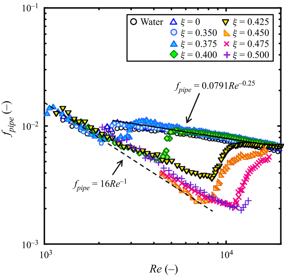
Figure 5. Friction coefficients depending on Reynolds number measured by the once-through flow system (Hidema et al. Reference Hidema, Suzuki, Hisamatsu, Komoda and Furukawa2013). The drag-reducing ability in a pipe was observed especially in solutions with ξ ≥ 0.4.
3.2. Vortex shedding at the comb influenced by high-order wormlike micellar structures
Figure 6 shows vortex shedding at the cylinder in each solution, which was visualized by interference patterns and instantaneous velocity fluctuations measured by PIV. These vortices merged with each other downstream of the flow and turned into a 2-D turbulent flow. The surfactant solution became viscoelastic with increasing ξ; thus, the water layer of the 2-D flow was slightly thickened. The interference patterns whitened at ξ ≥ 0.450. In the flow of the solutions with ξ ≥ 0.450, the vorticity obtained by the instantaneous velocity fluctuation was used to detect the vortices. The vortex visualized by the interference patterns corresponds well to the vorticity (Hidema et al. Reference Hidema, Murao, Komoda and Suzuki2018). Although the shapes of the vortices were not significantly varied by increasing ξ for ξ ≤ 0.450, from the interference patterns, the increase in small fluctuations in the vortices was visualized.

Figure 6. Interference patterns and instantaneous velocity fluctuation fields of vortex shedding at the comb. Interference patterns arising from the illumination light whiten in the solutions with ξ ≥ 0.450, which is caused by thickening of the water layer in the 2-D flow owing to an increase in the viscoelasticity of the solution. Although the interference patterns whiten, the velocity fields indicate that the vortices are shed at the comb at ξ = 0.45 as visualized by the vorticity. The colour bar shows the intensity of the vorticity. The expansion of the wake region is visualized by the vortices diminishing in the solutions with ξ ≥ 0.475.
The wake region that is the region behind the cylinder, within the area before the first vortex appears, suddenly expanded at ξ = 0.475 and higher ξ. The shape of the vortices varied at ξ = 0.475, and the vorticity was weakened. In the case of polyethyleneoxide (PEO)-doped flow, the variation in the vortices was affected by the relaxation time, λ, of the solutions. The relationship between λ and the characteristic time scale of vortex shedding, 1/f (s), determines the flow regimes, that is, the expansion of the wake region, diminishing of the vortices and regeneration of the vortices. Here, 1/f is obtained by the frequency of vortex shedding obtained by f = Uvortex/Lvortex, Uvortex (m s−1) is the vortex velocity and Lvortex (m) is the distance between two vortices that rotate in the same direction on the same side of the cylinder. The wake region expanded when 1/f > λ. The vortices almost disappeared in the region of 1/f ≈ λ. The vortices then appeared again in the region of λ > 1/f. These flow patterns and vortices are called vortex types 1, 2 and 3 in a previous study (Hidema et al. Reference Hidema, Fukushima, Yoshida and Suzuki2020).
However, in the case of the surfactant solution, the relationship between the characteristic time scale of the vortex shedding and relaxation time was not clear. Vortex types 1–3 were not clearly observed. In the surfactant solution with ξ ≤ 0.450, λ obtained by ODES-DOS was much shorter than 1 ms and the 1/f was approximately 10 ms. The Strouhal numbers obtained by f in each solution were approximately 0.2, which is similar to the original value. Therefore, the vortex shedding in the solution with ξ ≤ 0.450 was not significantly affected by the wormlike micelles. Conversely, the expansion of the wake region and vortex deformation were observed in solutions with ξ ≥ 0.475. The expansion of the wake region implies the formation of high-order wormlike micellar structures at the comb because of the high continuous extensional and shear stress around the cylinder in the flow. Here, we calculated the Weissenberg number of the solutions based on λ obtained by ODES-DOS and the mean extensional rates. The Weissenberg number was approximately 0.1–0.35, which was small. However, for the solutions with ξ ≥ 0.475, a structure that appeared to be highly viscoelastic appeared behind the cylinder. The structure grew in the wake region, where continuous extensional and shear stresses were applied, until it achieved a certain length. Then, it was detached from the cylinder. Subsequently, a new structure grew behind the cylinder. We assumed that the structure was the result of enhanced wormlike micelles promoted by the continuous extensional and shear stress in the flow. Here, we refer to the structure as a flow-induced structure. Furthermore, λ obtained by ODES-DOS may be much shorter than the relaxation time of the flow-induced structure. Therefore, it is reasonable to assume that the Weissenberg number calculated by the relaxation time of the flow-induced structure and the mean extensional rate may be much longer than the value calculated by the relaxation time of the solution and the mean extensional rate of 0.1–0.35.
3.3. Velocity fields around the comb
To clarify the energy transfer in the 2-D turbulent flow, the velocity fields close to the comb were observed and analysed using PIV. Figures 7(a)–7(c) show examples of instantaneous velocity fluctuations behind the cylinders in the surfactant solutions with ξ = 0.35–0.5. The vortices were shed just behind the comb in the solution with ξ = 0.350 (figure 7a). The vortices were slightly weakened in the solutions with ξ = 0.425 and 0.45, as shown in figures 7(b) and 7(c). A wake region appeared and the instantaneous velocity fluctuation approached 0 in the solutions with ξ = 0.475 and 0.5.
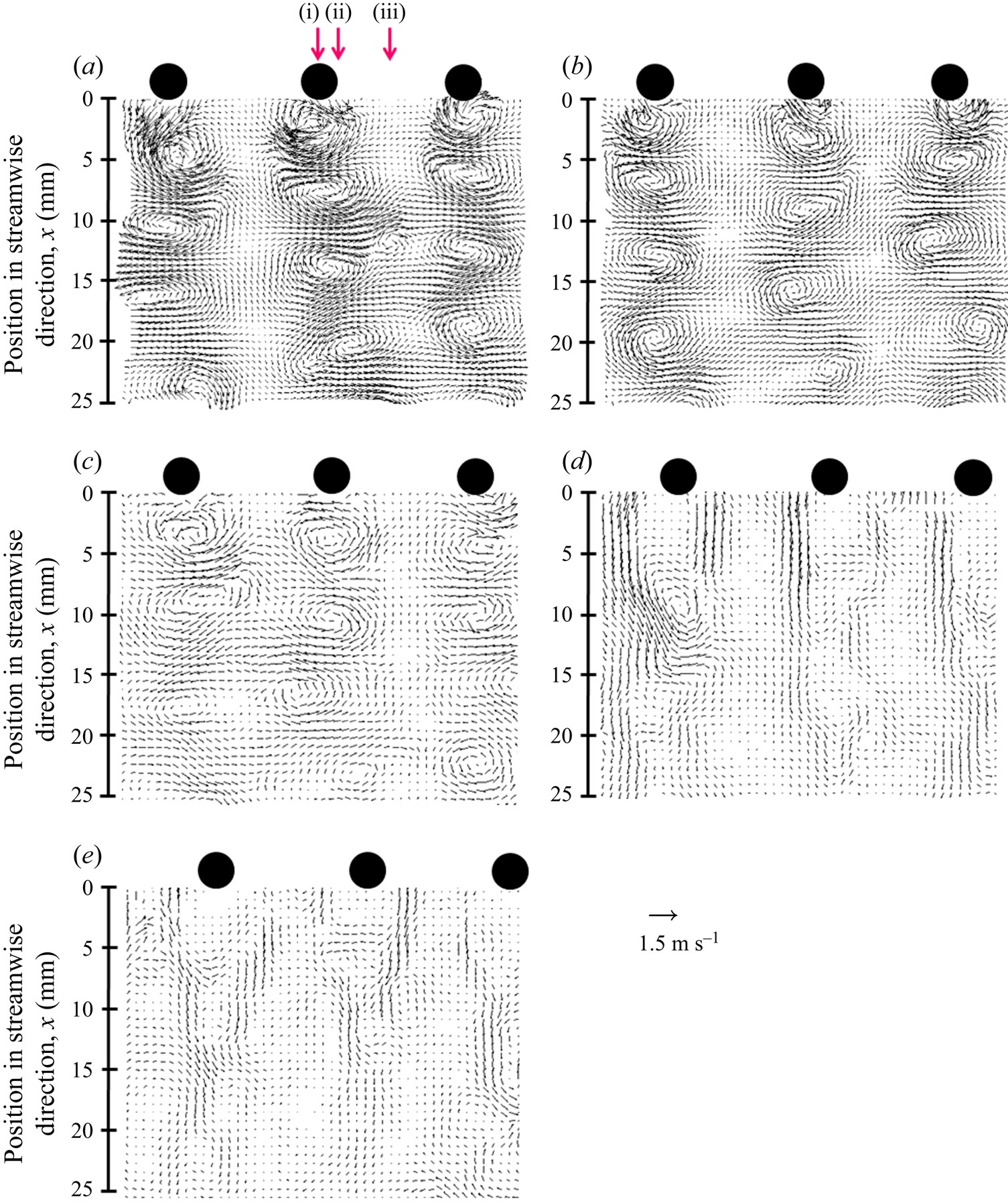
Figure 7. Instantaneous velocity fluctuation in the 2-D flow just behind the comb in the solutions with ξ = 0.35 (a), 0.425 (b), 0.45 (c), 0.475 (d) and 0.5 (e). The instantaneous velocity fluctuation at each local position is diminished, affected by the drag reduction ability of each sample solution. The three arrows in panel (a) indicate the downstream positions in the normal direction where k, P, D, ε, C and the budget are calculated. Positions (i), (ii) and (iii) correspond to the centre of the cylinder, the edge of the cylinder and the middle of two cylinders, respectively.
The local mean velocity  $\bar{U}_x$ in the streamwise direction at each downstream position is shown in figure 8. The local mean velocity is the time-average of the local velocity. The position in the normal direction was normalized by the distance between the cylinders. Thus, ‘0’ on the horizontal axis in figure 8 corresponds to the centre of the focused cylinder and ‘1’ on the axis corresponds to the centre of the neighbouring cylinder. The positive direction on the axis is downward, which corresponds to the flow direction. The local mean velocities largely varied in the normal and streamwise directions when ξ was low (figure 8a) and
  $\bar{U}_x$ continued to develop at 50 mm below the comb. The flow became viscoelastic with increasing ξ. Furthermore, the velocities behind the cylinders decreased and the velocity profiles became flat. The
  $\bar{U}_x$ approached the streamwise mean velocity Um quickly in solutions with ξ ≥ 0.475.

Figure 8. Development of the local mean velocity  $\bar{U}_x$ in the streamwise direction at each downstream position. The surfactant solution contains counter ions at concentrations of ξ = 0.35 (a), 0.425 (b), 0.45 (c), 0.475 (d) and 0.5 (e).
Figure 9 shows the contour of the local velocity gradient in the streamwise direction,  ${\rm d}\bar{U}_x/{\rm d}\kern0.06em x$, at each position in the flow. Here,
  $\bar{U}_x$ (m s−1) is the local mean velocity in the streamwise direction and
  ${\rm d}\kern0.06em x$ is the distance between the two grids in the calculation. The value of
  ${\rm d}\bar{U}_x/{\rm d}\kern0.06em x$ is closely related to the local extensional rate. In the case of the surfactant solutions with ξ = 0.35–0.45, the value of
  ${\rm d}\bar{U}_x/{\rm d}\kern0.06em x$ was high behind the cylinder. However, it changed to a negative value at a very close downstream position of approximately 10 mm. The distribution of
  ${\rm d}\bar{U}_x/{\rm d}\kern0.06em x$ differed in the solution with ξ = 0.475. The
  ${\rm d}\bar{U}_x/{\rm d}\kern0.06em x$ was virtually 0 s−1 just behind the cylinder and the maximum value was observed obliquely downward of the cylinder. In the case of the solution with ξ = 0.5,
  ${\rm d}\bar{U}_x/{\rm d}\kern0.06em x$ was virtually 0 s−1 just behind the cylinder and the value gradually increased with increasing distance from the cylinder. For the solutions with ξ = 0.475 and 0.5, a positive value for
  ${\rm d}\bar{U}_x/{\rm d}\kern0.06em x$ was observed farther downstream. A positive value was also observed in the area between the two cylinders. The different characteristics of
  ${\rm d}\bar{U}_x/{\rm d}\kern0.06em x$ may arise from the flow-induced structure around the cylinder in the solutions with ξ = 0.475 and 0.5. The presence of the flow-induced structure may cause an increase in the local extensional viscosity of the solution, which induces a long wake region behind the cylinder. Furthermore, the structure relaxes slowly and influences the turbulent statistics, as described in § 3.4.
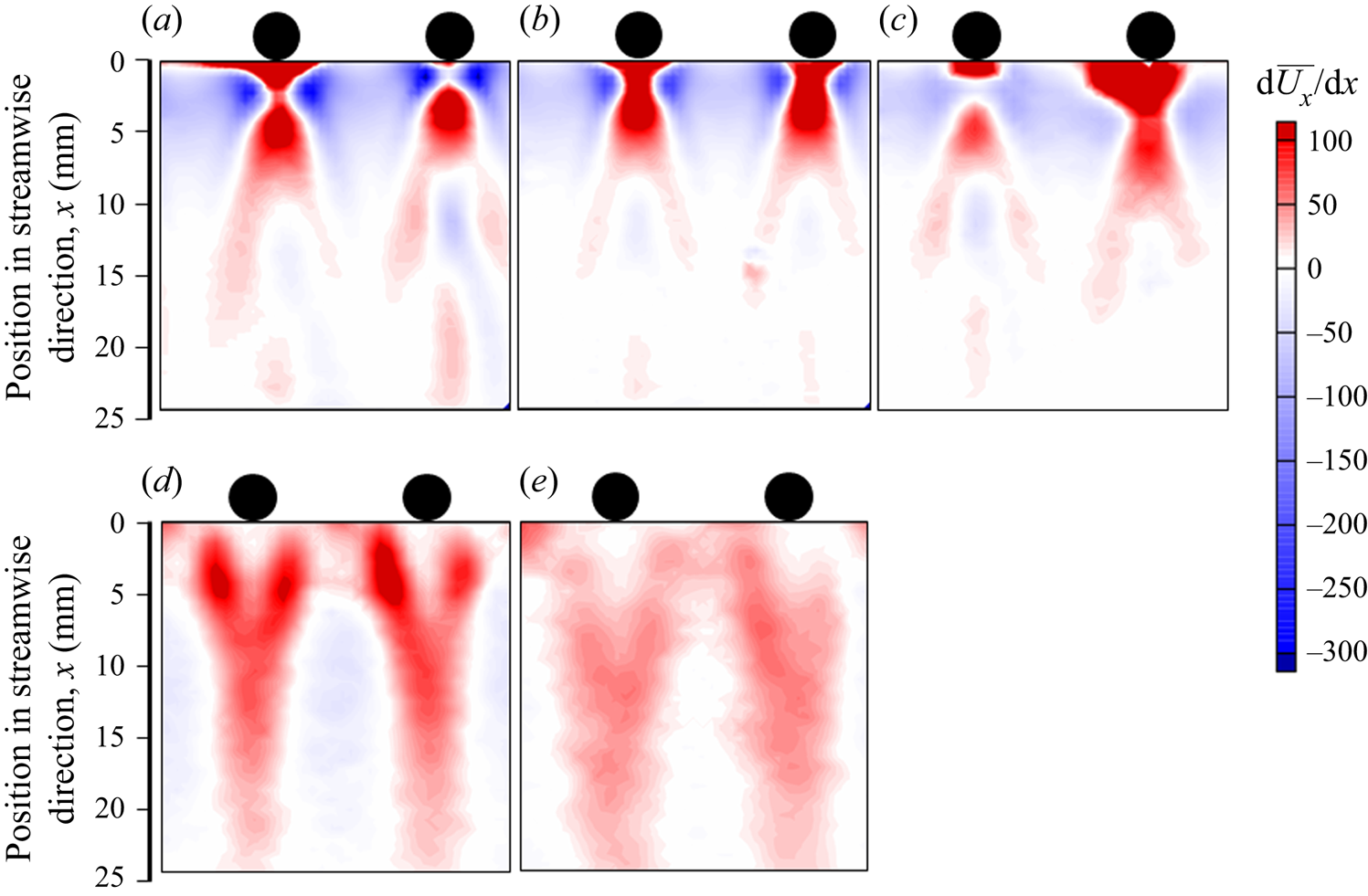
Figure 9. Contour of  ${\rm d}\bar{U}_x/{\rm d}\kern0.06em x$ in the 2-D flow close to the comb with ξ = 0.35 (a), 0.425 (b), 0.45 (c), 0.475 (d) and 0.5 (e).
3.4. Fluctuation intensity and Reynolds stress
The fluctuation intensities in the normal and streamwise directions were calculated using  $u_{i\,rms}/U_m$. Figure 10 shows the fluctuation intensity in the normal direction,
  $u_{y\,rms}/U_m$, of each solution at each downstream position. The horizontal axis denotes the normalized position in the normal direction. The fluctuation intensities gradually decreased with the distance from the comb for ξ < 0.425, as shown in figures 10(a) and 10(b). However, the distance from the comb at which
  $u_{y\,rms}/U_m$ showed a higher value shifted downstream with increasing ξ. Furthermore,
  $u_{y\,rms}/U_m$ became flat at a certain distance from the comb by increasing ξ, as shown in figures 10(d) and 10(e).

Figure 10. Fluctuation intensities in the normal direction for sample solution with ξ = 0.35 (a), 0.425 (b), 0.45 (c), 0.475 (d) and 0.5 (e).
Figure 11 shows the fluctuation intensities in the streamwise direction,  $u_{x\,rms}/U_m$. The
  $u_{x\,rms}/U_m$ split into two peaks around the cylinders when ξ was smaller (figures 11a–11c). The
  $u_{x\,rms}/U_m$ was smaller than
  $u_{y\,rms}/U_m$ when ξ was small, which corresponds to the flow regimes in which round vortices were shedding strongly from side to side of the cylinder. However, the
  $u_{x\,rms}/U_m$ profile changed drastically at ξ = 0.475. Just behind the cylinder,
  $u_{x\,rms}/U_m$ became almost zero and
  $u_{x\,rms}/U_m$ became flat downstream. The measured fluctuation at the downstream position in the solution with a high ξ was larger than that in the solution with a lower ξ and was more noticeable in the streamwise direction (figures 11d and 11e). This feature indicates the anisotropy of the flow of the drag-reducing surfactant solution owing to the formation of high-order wormlike micellar structures at the comb. As shown in figure 9, extensional flow occurring in the flow enhanced the formation of the wormlike micellar structure, i.e. the flow-induced structure, which led to a long wake region behind the cylinder. The flow-induced structure relaxed slowly and maintained the fluctuation farther downstream.

Figure 11. Fluctuation intensities in the streamwise direction for sample solutions with ξ = 0.35 (a), 0.425 (b), 0.45 (c), 0.475 (d) and 0.5 (e).
Figure 12 shows the Reynolds stress calculated using (2.2). The Reynolds stress decreased with increasing distance from the comb and quickly diminished with increasing ξ.

Figure 12. Reynolds stress values for sample solutions with ξ = 0.35 (a), 0.425 (b), 0.45 (c), 0.475 (d) and 0.5 (e).
3.5. Turbulent energy characteristics
The turbulence statistics of the 2-D flow were calculated based on the local velocity fields measured by the PIV. Figure 13 displays the turbulent energy k and its development in the streamwise direction calculated using (2.3). In the figure, k is normalized by the streamwise mean velocity, Um. The position in the normal direction is located just behind the cylinder, at the edge of the cylinder and in the middle of the two cylinders, as indicated in figure 7(a) by positions (i), (ii) and (iii), respectively. The k development varied considerably with position and ξ. At position (i), k increased just behind the cylinder in the solution with ξ = 0.35 and gradually decreased with the distance from the cylinder. The maximum value of k decreased with an increase in ξ for ξ < 0.45. The increase in k was delayed in the solution with ξ = 0.475 and no specific peak was observed at a distance of 25 mm from the cylinder (figure 13a). This feature was particularly noticeable in the solution with ξ = 0.5 and k reached a higher value. At position (ii), the maximum value of k decreased in the solution with ξ ≤ 0.45 and a specific peak was not observed. The tendency observed at position (i) in the solutions with ξ = 0.475 and 0.5 was clearly seen at position (ii).
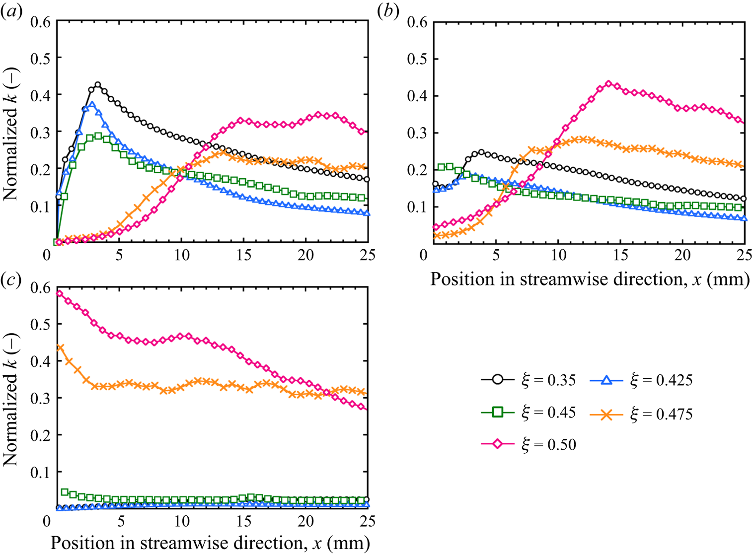
Figure 13. Normalized k in the turbulent flow of each sample solution in the streamwise direction. Panels (a) to (c) indicate the normalized k at positions (i) to (iii), respectively.
At position (iii), although the value of k was low in the solution with ξ ≤ 0.45, k reached a much higher value in the solutions with ξ = 0.475 and 0.5. Figure 14 shows the contour of k around the comb in each solution and clearly shows that k increased in the area between the cylinders in the solution with ξ = 0.5. This feature is very different from that of a polyethylene oxide (PEO) drag-reducing solution (Hidema et al. Reference Hidema, Fukushima, Yoshida and Suzuki2020). In the case of the PEO solution, the maximum value of k was observed at position (i). Conversely, in the case of the drag-reducing surfactant solution, the flow-induced structure formed just behind the cylinder in the solution with a high ξ, which decreased the local velocity at position (i). The decrease in the local velocity behind the cylinder led to an increase in the local velocity between the cylinders, which caused an increase in k at position (iii).

Figure 14. Contour of k around the comb in each surfactant solution. Here, only two cylinders in the comb are chosen with ξ = 0.35 (a), 0.425 (b), 0.45 (c), 0.475 (d) and 0.5 (e).
To consider the origin of k, the values of P, ε and D of the turbulent energy were calculated using (2.5)–(2.7). Figure 15 shows P, D and ε of each sample solution in the streamwise direction at position (i). These values were normalized using Um and the cylinder diameter. In the case of the surfactant solution with ξ = 0.35, the distance from the cylinder where the peak appeared in k, lk-peak, and the distance where the peak appeared in P were the same. Thus, the k of the solution that does not have drag reduction ability originates from P in turbulent flow. A similar tendency was observed in the solutions with ξ = 0.425 and 0.45, which had a lower effect on drag reduction than those with ξ = 0.475 and 0.5.

Figure 15. Normalized P, D, ε and budget of the surfactant solutions with ξ = 0.35 (a), 0.425 (b), 0.45 (c), 0.475 (d) and 0.5 (e) at position (i).
The maximum value of P decreased with an increase in ξ. In the case of the highly drag-reducing surfactant solutions with ξ = 0.475 and 0.5, although k was high, P, D and ε were zero. Therefore, the peak observed for k in these solutions cannot be explained by the turbulent energy transfer of Newtonian fluids. This implies that the peak value of k observed in the surfactant solution originates from the relaxation phenomenon of the wormlike micelle solution. The relaxation time of the sample solution detected by the ODES-DOS was very small for ξ < 0.5. However, the solution formed a flow-induced structure at the cylinder, which was caused by the enhanced wormlike micellar structure. The structure may induce longer relaxation times, which affect the value of k in the surfactant solutions with ξ = 0.475 and 0.5. The flow-induced structure appeared just behind the cylinder and slowly diminished downstream, which may have affected the slow relaxation of k, as shown in figure 17.
To confirm the accuracy of the measurements and calculations in this study, the budget described in (2.9) is shown in figure 15. For the surfactant solutions with ξ = 0.35 and 0.425, the budget was not close to zero in the wake region. This was a consequence of 3-D flow disturbance. Here, the local velocities  $U_i$ in the streamwise and normal directions were measured and calculated using PIV. However, at the position immediately behind the cylinder, the flow fluctuated in the spanwise direction. This fluctuation induced a budget. However, the budget converged to virtually zero at 10 mm from the comb. The budget was virtually zero for the solutions with ξ > 0.425. The viscoelasticity of the solutions with high ξ prohibited fluctuations in the spanwise direction.
To confirm that the increase in k at positions (i)–(iii), as shown in figure 13, was not owing to the turbulent energy production and diffusion produced at different locations in the flow, P, D, ε and the budget at positions (ii) and (iii) were calculated. Figure 16 shows the normalized P, D, ε and budget in the solutions with ξ = 0.35 and 0.5 at each position. In the case of the solution with ξ = 0.35, an increase in P was observed at position (ii); however, the value was smaller than that observed at position (i). P, D, ε and the budget of the solution with ξ = 0.35 at position (iii) and of the solution with ξ = 0.5 at positions (ii) and (iii) were virtually zero. Thus, the increase in k at positions (i)–(iii) was not transported from the different locations.

All the features shown in figures 13–16 suggest that the origin of k is not owing to the production of the Newtonian turbulent flow but imply the effect of elastic turbulence. Groisman & Steinberg (Reference Groisman and Steinberg2000) suggested the elastic turbulence that an elastic polymer solution at a sufficiently high Weissenberg number induces the characteristic behaviours observed in turbulent flow. The stretching of the polymer and its slow relaxation generate elastic stress, which contributes to the flow resistance in elastic turbulence. It is possible that the high value of k observed in the flow of the solutions with ξ = 0.475 and 0.5 arises from the generation of elastic turbulence caused by a flow-induced structure that may have a long relaxation time. Contribution of elastic energy in k can be positive and negative in the flow, which may be dependent on the position from the comb. However, this hypothesis requires further consideration, which will be the focus of a future study.
The large value of k that may arise from the flow-induced structure was maintained farther downstream. This is clearly shown in figure 17, which shows the k values in the solution with ξ = 0.5 at position (i). In the case of PEO-doped 2-D turbulent flow, the distance from the cylinder where the peak appeared in k, lk-peak, was related to the relaxation time measured by the CaBER (Hidema et al. Reference Hidema, Fukushima, Yoshida and Suzuki2020), which implies that the extension and relaxation of polymers in the turbulent flow affected the transfer of energy. In contrast, in the case of the drag-reducing surfactant solution, the lk-peak was not related to the relaxation time measured by ODES-DOS. However, the large k maintained downstream implies the contribution of the flow-induced structure, which may have a longer relaxation time, to the turbulent flow behaviour.

Figure 17. Normalized k farther downstream in the solution with ξ = 0.5.
4. Conclusion
An experimental study was performed to investigate the effects of the extensional rheological properties of drag-reducing surfactant solutions on vortex shedding in 2-D turbulent flow and turbulence statistics.
ODES-DOS measurements were used to determine the relaxation times of the surfactant solutions. The relationship between the vortex shedding time and the relaxation time measured by ODES-DOS was not as clear for the wormlike micelle solution as it was for the drag-reducing polymer solution. However, the extensional and shear rates applied to the solution around the cylinder in the 2-D flow resulted in the formation of an enhanced wormlike micellar structure, which we call a flow-induced structure. The flow-induced structure drastically changed the vortex shedding, velocity development and turbulence statistics in the solutions with ξ = 0.475 and 0.5.
In particular, the high value of turbulent energy k that was maintained downstream in the solutions with ξ = 0.475 and 0.5 was a characteristic feature of the drag-reducing surfactant solution. The characteristic k appeared without an increase in the turbulent energy production P calculated by the equation for Newtonian fluids. This phenomenon implies a longer relaxation time of the flow-induced structure, which may contribute to the generation of elastic turbulence. This hypothesis will be investigated in a future study.
Funding
The present study was supported in part by a Grant-in-Aid for Scientific Research (B) (Project No. 19H02497), a grant for Challenging Research (Exploratory) (Project No. 19K22083) from the Japan Society for the Promotion of Science (JSPS KAKENHI) and a grant for Fusion-Oriented-Research-for-disruptive-Science- and-Technology (FOREST) from the Japan Science and Technology Agency.
Declaration of interests
The authors report no conflicts of interest.


