Genotype × Environment (G × E) Interactions
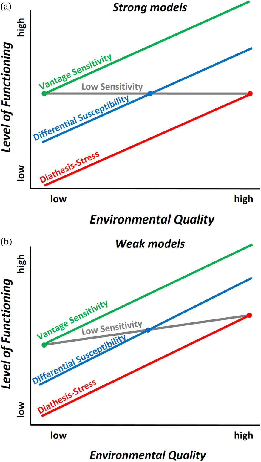
Over the past 15 years, several distinct conceptual models of how individual and environmental characteristics interact in shaping development have been used in studying and interpreting evidence of G × E. These models include (a) diathesis-stress, stipulating that some individuals carry “risk” genes that make them disproportionately susceptible to adverse environmental conditions (Zubin & Spring, Reference Zubin and Spring1977); (b) vantage sensitivity, stipulating that some individuals disproportionately benefit from supportive conditions due to their genetic makeup (Pluess & Belsky, Reference Pluess and Belsky2013); and (c) differential susceptibility, stipulating that some individuals are more developmentally plastic “for better and for worse” (Belsky, Bakermans-Kranenburg & van IJzendoorn, Reference Belsky, Bakermans-Kranenburg and Van IJzendoorn2007), being more susceptible to both negative effects of adversity and beneficial effects of support (Belsky, Reference Belsky1997a, Reference Belsky1997b), thus reconceptualizing would-be “risk” genes into more general “plasticity” or “sensitivity” genes. Weak and strong versions of each model can be envisioned; in strong models, some individuals are affected by the environmental exposure of interest while others are not, whereas in weak models all are affected by the environmental exposure, but some more strongly than others. See Figure 1 for a graphical representation of the (a) strong and (b) weak models.

Figure 1. A graphical representation of the three G×E hypotheses tested (vantage sensitivity, differential susceptibility, and diathesis-stress) and where the crossover point is situated in each case assuming a) weak and b) strong models.
Most work evaluating diverse models of G × E interaction has been exploratory in character, failing to formally evaluate which model fit the data best (see Assary, Vincent, Keers, & Pluess, Reference Assary, Vincent, Keers and Pluess2017, for a recent review of the subject). Kochanska, Kim, Barry, and Philibert (Reference Kochanska, Kim, Barry and Philibert2011) were the first to use the now classical regions of significance (RoS) analysis (Aiken, West, & Reno, Reference Aiken, West and Reno1991; Hayes & Matthes, Reference Hayes and Matthes2009; Preacher, Curran, & Bauer, Reference Preacher, Curran and Bauer2006) to differentiate diathesis-stress from differential susceptibility. Assuming a single binary genetic variant (e.g., short vs. long serotonin transporter linked polymorphic region [5-HTTLPR] allele), the RoS approach determines the range of values of the environment where the environment-predicting outcome regression lines significantly differ from each other. A G × E model is considered to reflect diathesis-stress when the lines are significantly different only in the lower observable range of the environmental quality measure (e.g., poor parenting), thereby reflecting adversity; vantage sensitivity when the lines are significantly different only in the upper observable range of the environmental quality measure (e.g., good parenting), thereby reflecting support of enrichment; and differential-susceptibility when the lines are significantly separated at both ends of the environmental quality measure. See Figure 2 for a graphical representation of the (a) diathesis-stress model, (b) differential susceptibility model, and (c) vantage sensitivity model with the RoS.

Figure 2. A graphical representation of the three G×E hypotheses tested (vantage sensitivity, differential susceptibility, and diathesis-stress) and the regions of significance (in grey; area where the slopes are significantly different from one another).
In seeking to advance new methods for empirically distinguishing different conceptual models of G × E interaction, Roisman et al. (Reference Roisman, Newman, Fraley, Haltigan, Groh and Haydon2012) highlighted several limitations of the RoS approach. Because statistical significance is a function of sample size, larger studies would be more likely to detect significantly different slopes in both the lower and the upper ends of the spectrum than smaller ones. In addition, the RoS approach is likely sensitive to Type 1 errors, particularly when testing multiple variants and environments. For example, if one has 10 genetic variants and 5 environmental measures, one could conduct 10 × 5 = 50 pairwise tests. Assuming testing at the 5% level (i.e., p value < .05; 95% confidence interval), the probability of having at least one false positive out of 50 tests is 92.3%. Such multiple testing means that the confidence intervals should be adjusted to allow for the consideration of multiple hypotheses in the same empirical effort. However, in practice, many researchers do not adjust for multiple testing, let alone report their nonsignificant results (Earp & Trafimow, Reference Earp and Trafimow2015; Simmons, Nelson, & Simonsohn, Reference Simmons, Nelson and Simonsohn2011). Finally, as a result of nonlinearity, the slopes might never cross even when they are significantly different given the observable range of the environmental variable.
About the same time that Roisman et al. (Reference Roisman, Newman, Fraley, Haltigan, Groh and Haydon2012) were expressing the concerns just raised, Widaman et al. (Reference Widaman, Helm, Castro-Schilo, Pluess, Stallings and Belsky2012; Belsky, Pluess, & Widaman, Reference Belsky, Pluess and Widaman2013) proposed a method for competitively evaluating the fit of diathesis-stress and differential-susceptibility models of G × E, one which was confirmatory rather than exploratory. In their competitive-confirmatory approach, the crossover point is the critical parameter. Whereas the diathesis-stress model is constructed by fixing the crossover point at the higher end of the environmental quality spectrum, the differential-susceptibility model is constructed by treating the crossover point as an unknown parameter to be estimated. A simple adjustment to the Widaman et al. approach would also enable it to evaluate vantage sensitivity, by fixing the crossover point at the lower end of the environmental quality spectrum. Criteria such as the Akaike information criterion or the Bayesian information criterion (BIC) can be used to determine which alternative model fits the data best. Of note, this competitive-confirmatory approach still relies indirectly on hypothesis testing, but only for the purpose of rejecting models of differential susceptibility that have a confidence interval for the crossover point that lies outside the observable range. To date, these models have been used principally in studies focused on a single candidate gene and a single environmental exposure.
Multiple Genes and Environments
As mentioned by Roisman et al. (Reference Roisman, Newman, Fraley, Haltigan, Groh and Haydon2012), the risk of Type 1 errors in G × E testing approaches is high considering that one needs to run separate analyses for each individual pair of gene/environment variables. This problem is even more relevant and pronounced in the era of big data when the cost of DNA sequencing has rapidly decreased and become more affordable in large-scale epidemiological research (Wetterstrand, Reference Wetterstrand2016). Another problem with single-gene and single-environment G × E models is that most G × E models involving single genes and single environments have very small effect sizes and low replication rates (Lee et al., Reference Lee, Perlis, Jung, Byrne, Rueckert, Siburian and Pergadia2012; Risch et al., Reference Risch, Herrell, Lehner, Liang, Eaves, Hoh and Merikangas2009). This is not surprising based on the common understanding that most phenotypes are affected by multiple genes, to say nothing of multiple environments.
These considerations highlight the need to develop G ×E approaches that can handle multiple genes and/or multiple environments, which was the reason we developed an approach using alternating optimization (Jolicoeur-Martineau et al., Reference Jolicoeur-Martineau, Wazana, Székely, Steiner, Fleming, Kennedy and Greenwood2017) to construct a Genetic Score (g) × Environmental Score (e) model, in which g is a weighted sum of the genetic variants and e is a weighted sum of the environments. This approach estimates, in turn, the weights of the G × E model, the weights of the genetic score and the weights of the environmental score. We call the models fitted using this approach Latent Environmental and Genetic InTeraction (LEGIT) models.
With this approach, instead of testing the interaction of each gene/environment pair (n_genes × n_env tests), one has to test only once for the presence of a Genetic Score × Environmental Score interaction. How much each genetic/environmental variable contributes to its corresponding genetic/environmental score can then be tested for each individual variables (n_genes + n_env tests); however, this latter is not required to test for the presence of a significant G × E. We recommend that instead of making a decision based on p values of the G × E term, one should rather compare the BIC of the models with and without an interaction term; doing so renders false positives very unlikely (as is shown in the Results section). We wish to emphasize the distinction between (a) the testing of multiple genes and environments in serial models, and (b) the use of a model that fits, within set parameters of genes and environments established a priori, the optimal weights for each term of the equation. The vast majority of statistical models used in the developmental-behavioral sciences (e.g., mixed models, logistic regression, and structural equation models) use the latter, with an iteration-based optimization approach to estimate the parameters. Thus, our alternating optimization is no different from analytic approaches commonly used in our field of research.
Here we seek to extend this initial work by adapting and applying RoS and the competitive-confirmatory approaches within LEGIT models to test for the pattern of interaction between the genetic and environmental score. This affords the differentiation of differential susceptibility, diathesis-stress, and vantage sensitivity in a multigene/multienvironment G × E setting.
In an effort to extend work evaluating alternative G × E models, we evaluate, via simulation, the relative accuracy of the RoS and competitive-confirmatory approaches under a wide range of scenarios; these include single and multiple genes, single and multiple environmental measures, different effect sizes, different sample sizes, symmetric and skewed distributions of the environment, and crossover points at 25% or 50% of the measured environmental quality range.
Below, we first briefly review the RoS, competitive-confirmatory, and alternating optimization approaches. Next, we discuss how to combine the RoS and competitive-confirmatory approaches with alternating optimization. Finally, we use statistical simulations to test whether
1. Confirmatory and competitive testing has differential accuracy in determining the pattern of G × E for small sample sizes and effect sizes compared to RoS.
2. Our method combining competitive-confirmatory and alternating optimization approaches has good accuracy in a multi G × E model (i.e., four genetic variants and three environmental measures) assuming (a) a moderate effect size and large sample size (i.e., N = 500 or greater) or (b) a large effect size and small to moderate sample size (i.e., N = 250 or greater).
Method
G × E model definition
A standard G × E model can be represented in the following way:
 $${\bi y} = \beta _0 + \beta _e{\bi e} + \beta _g{\bi g} + \beta _{eg}{\bi eg} + {\bf \varepsilon}, \, $$
where yis a vector representing the n observed outcomes, β 0 is the intercept, β e the regression weight for the environment main effect (e), β g the regression weight for the gene main effect (g), and β eg is the regression weight for the product of environment and genes (eg), which represents the G × E interaction. For a fitted model, we use the following formulation:
 $$E\lsqb {{\bi y} \vert {\bi e}\comma \,{\bi g}} \rsqb = {\hat \beta} _0 + {\hat \beta} _e{\bi e} + {\hat \beta} _g{\bi g} + {\hat \beta} _{eg}{\bi eg}.$$
The hat (^) is used on top of parameters to represent that these are estimated parameters rather than the original ones. This notation will be used through the paper.
Simple slopes and RoS
Assuming a single binary genetic variant (e.g., short vs. long 5-HTTLPR allele), a G × E model has two environment-predicting outcome regression lines: one representing individuals with, putatively, low environmental sensitivity and another representing individuals with, putatively, high environmental sensitivity. The traditional approach for distinguishing between differential susceptibility, diathesis-stress, and vantage sensitivity is to determine at which values of the environment the lines differ significantly from each other.
To this end, one must first reparametrize a G × E model as an explicit function of the genotype:
 $$\displaylines{E\lsqb {{\bi y} \vert {\bi e}\comma \,{\bi g}} \rsqb = {{\hat \beta}} _0 + {{\hat \beta}} _e{\bi e} + {{\hat \beta}} _g{\bi g} + {{\hat \beta}} _{eg}{\bi eg} \cr \qquad \qquad \hskip5pt = \lpar {{{\hat \beta}}_0 + {{\hat \beta}}_e{\bi e}} \rpar + ({{\hat \beta}} _g + {{\hat \beta}} _{eg}{\bi e}){\bi g} \cr \hskip-23pt = {{\hat w}}_0 + {{\hat w}}_1{\bi g}.} $$
We call ŵ 0 the simple intercept and ŵ 1 the simple slope. The simple slope represents the slope as a function of g. This means that if ŵ 1 is significantly different from zero, then the slopes for different values of g (e.g., the slopes for g = 0 and g = 1 if g is dichotomous) are significantly different from one another.
The variance of the simple slope is
 $$\displaylines{Var\lsqb {{{\hat w}}_1 \vert {\bi e}} \rsqb = Var\lpar {{{\hat \beta}}_g} \rpar + Var\lpar {{{\hat \beta}}_{eg}{\bi e}} \rpar + 2Cov\lpar {{{\hat \beta}}_g\comma \,{{\hat \beta}}_{eg}{\bi e}} \rpar \; \; \cr \hskip3.6pc = Var\lpar {{{\hat \beta}}_g} \rpar + {\bi e}^2Var\lpar {{{\hat \beta}}_{eg}} \rpar + 2{\bi e}Cov\lpar {{{\hat \beta}}_g\comma \,{{\hat \beta}}_{eg}} \rpar .} $$
Using standard regression asymptotic theory (Aiken et al., Reference Aiken, West and Reno1991), it can be shown that
 $$\displaystyle{{{{\hat w}}_1} \over {\sqrt {Var\lsqb {{{\hat w}}_1 \vert {\bi e}} \rsqb }}} \sim t_{N-5},$$
where t N-5 is a student's t distribution with N – 5 degrees of freedom (df) and N is the number of observations.
Based on the above equations, it is possible to test whether the simple slope is significantly different from zero, and thus determine if the slopes for different values of g are significantly different from one another at fixed values of e. However, this does not tell us at which values of e is ŵ 1 significant. The Johnson–Neyman technique (Johnson & Fay, Reference Johnson and Fay1950) uses this formula, in a backward fashion, to find the range of values of e where the simple slope is significantly different from zero. This range corresponds to the RoS, and it can be defined by a lower bound L and an upper bound U. When e is larger than L and smaller than U, the slopes for different values of g do not differ significantly, whereas outside these bounds they do.
Kochanska et al. (Reference Kochanska, Kim, Barry and Philibert2011) suggested using RoS (Aiken et al., Reference Aiken, West and Reno1991; Hayes & Matthes, Reference Hayes and Matthes2009; Preacher et al., Reference Preacher, Curran and Bauer2006) to help differentiate diathesis-stress from differential susceptibility. When the RoS are within the observable ranges of values for e, the data are considered to reflect differential susceptibility. When only the lower bound L of the RoS is within the observable range, the data is considered to reflect diathesis-stress. When only the upper bound U of the RoS is within the observable range, the data is considered to reflect vantage sensitivity. If neither L nor U is within the observable range, results are inconclusive.
Confirmatory and competitive models
As shown above, the RoS approach focused entirely on the lower and upper bounds of the RoS. An alternative point of view is to focus instead on the crossover point, the point where the slopes for the different values of the environment cross. It was shown (Aiken et al., Reference Aiken, West and Reno1991; Widaman et al., Reference Widaman, Helm, Castro-Schilo, Pluess, Stallings and Belsky2012) that the crossover can be found using the following formula:
 $$c = -\displaystyle{{\beta _g} \over {\beta _{eg}}}.$$
Similarly to the RoS approach, if the complete 95% confidence interval of the crossover point is within the observable range of the environment, it is suggestive of differential susceptibility. To obtain a confidence interval for the crossover point, Widaman et al. (Reference Widaman, Helm, Castro-Schilo, Pluess, Stallings and Belsky2012) suggested fitting a model where the crossover point c is an unknown parameter to be estimated. The authors showed that the standard G × E formulation (1) can be reparametrized as
 $${\bi y} = \beta _0 + \beta _e\lpar {{\bi e}-c} \rpar + \beta _{eg}\lpar {{\bi e}-c} \rpar {\bi g} + {\bf \varepsilon}.$$
Although β g does not appear in this equation, Widaman et al. (Reference Widaman, Helm, Castro-Schilo, Pluess, Stallings and Belsky2012) have shown that this parametrization is equivalent due to the inclusion of the crossover point c.
Using nonlinear regression estimation, Model 5 can be fitted and the crossover point can be estimated directly along with its confidence intervals. It is important to note that the estimate of the crossover point is not normally distributed (Lee, Lei, & Brody, Reference Lee, Lei and Brody2015; Marsaglia, Reference Marsaglia1965), suggesting that the resulting confidence interval may be biased. However, it has been shown that when the sample size is large enough (N > 500), the crossover point is approximately normally distributed (Lee et al., Reference Lee, Lei and Brody2015; Marsaglia, Reference Marsaglia1965). In addition, even when the sample size is small, the nonnormality of the crossover point does not lead to significant problems in the case of the competitive-confirmatory approach, as it does not rely exclusively on confidence intervals to distinguish between differential susceptibility and diathesis-stress; this is in contrast to the RoS approach. Instead, Widaman et al. (Reference Widaman, Helm, Castro-Schilo, Pluess, Stallings and Belsky2012) constructed confirmatory and competitive models of differential susceptibility and diathesis-stress to determine which model best fits the data. In accordance, the purpose of the confidence interval of the crossover point is only to verify that the crossover point is within the observable range of the environment when a differential susceptibility model is deemed to be the best fit-wise. To prevent any confusion, we will use the notation c for the true crossover point, ĉ for the estimated crossover of the differential susceptibility models, c low for the crossover point of the vantage sensitivity models, and c high for the crossover point of the diathesis-stress models.
Although the original paper by Widaman et al. (Reference Widaman, Helm, Castro-Schilo, Pluess, Stallings and Belsky2012) focused only on the diathesis-stress and differential susceptibility models, we extend this approach in the current effort by also presenting the vantage sensitivity models. Furthermore, we extend all concepts to situations where multiple environmental variables contribute to an environmental score, and where multiple genetic variables contribute to a genetic score. Accordingly, there are six models tested in our extension to multidimensional situations:
1. weak vantage sensitivity (β e estimated, c low = min(e))
2. strong vantage sensitivity (β e = 0, c low = min(e))
3. weak differential susceptibility (β e estimated, c estimated)
4. strong differential susceptibility (β e = 0, c estimated)
5. weak diathesis-stress (β e estimated, c high = max(e))
6. strong diathesis-stress (β e = 0, c high = max(e))
All six models are constructed using Equation 4. The models of differential susceptibility (Models 3 and 4) need to estimate an extra parameter, namely, the crossover point; therefore, Widaman et al. (Reference Widaman, Helm, Castro-Schilo, Pluess, Stallings and Belsky2012) suggested using the Akaike information criterion (Akaike, Reference Akaike, Akaike, Parzen, Tanabe and Kitagawa1998) or the BIC (Schwarz, Reference Schwarz1978) to evaluate the quality of fit.
Latent genetic and environmental score models
Instead of considering a linear regression on a single observed genetic variant and environment, as in Equation 1, Jolicoeur-Martineau et al. (Reference Jolicoeur-Martineau, Wazana, Székely, Steiner, Fleming, Kennedy and Greenwood2017) instead considered a linear regression on latent genetic (g) and environmental (e) scores and their interaction. These latent scores are defined as the weighted sum of their corresponding variables (genetic or environmental). The goal thus becomes not only to estimate the parameters of the G × E but also to estimate the weights of the genetic and environmental variables that make up the latent variables. Jolicoeur-Martineau et al. (Reference Jolicoeur-Martineau, Wazana, Székely, Steiner, Fleming, Kennedy and Greenwood2017) defined their model in three parts: the genetic score g, the environmental score e, and the main model.
 $$\eqalign{{\bi g} & = \mathop \sum \limits_{\,j = 1}^k p_j {\bi g}_j \cr {\bi e} &= \sum \limits_{l = 1}^s q_l {\bi e}_l \cr & y = \beta _0 + \beta _e {\bi e} + \beta _g {\bi g} + \beta _{eg} {\bi eg} + {\bf \varepsilon}\comma} $$
where p = (p 1, p 2, … , p k) is a vector of parameters for the k genetic variables g1, g2, … , gk and q = (q 1, q 2, … , q s) is a vector of parameters for the s environmental variables e1, e2, … , es.
Note that there are infinitely many possibilities for p and q that lead to the same model. For example, β e, β eg with Cp, where C is a constant, leads to the exact same model as C β e, Cβ eg with p:
 $$\eqalign{& y = \beta _0 + \beta _e {\bi e} + \beta _g \sum \limits_{\,j = 1}^k (Cp_j) {\bi g}_j + \beta _{eg}{\bi e} \sum \limits_{\,j = 1}^k (Cp_j) {\bi g}_j + {\bf \varepsilon} \cr & = \beta _0 + \beta _e {\bi e} + C\beta _g \sum \limits_{\,j = 1}^k p_j {\bi g}_j + C\beta _{eg}{\bi e} \sum \limits_{\,j = 1}^k p_j {\bi g}_j + {\bf \varepsilon} \cr & = \beta _0 + \beta _e{\bi e} + (C\beta _g){\bi g} + (C\beta _{eg}){\bi eg} + {\bf \varepsilon}.} $$
To prevent infinite possibilities for p and q, the following restrictions are added:
 $$\matrix { {\mathop \sum \limits_{\,j = 1}^k \vert {\,p_j} \vert = 1\comma \,} \hfill \cr {\; \mathop \sum \limits_{l = 1}^s \vert {q_l} \vert = 1.} \hfill \cr} $$
This restriction also aids interpretation because the weights of the genetic and environmental scores represent the relative contribution of the individual genetic variants and environmental variables to their respective composites.
To estimate the weights of the genetic score, the environmental score, and the main models, an alternating optimization approach is used. We first initialize p to (1/k, 1/k, … , 1/k) and q to (1/s, 1/s, … , 1/s), that is, we assume that all genetic and environmental variables are equally weighted; this is equivalent to taking the average of all the genetic or environmental variables. Then, the approach comprises three steps: (a) estimating β 0, β e, β g, β eg assuming that p and q are known, (b) estimating p assuming that q and β 0, β e, β g, β eg are known, and (c) estimating q assuming that p and β 0, β e, β g, β eg are known (Jolicoeur-Martineau et al., Reference Jolicoeur-Martineau, Wazana, Székely, Steiner, Fleming, Kennedy and Greenwood2017). This is done in iterative steps until convergence, at each step ensuring that the parameters of the genetic and environmental scores sum to one in absolute values (constraints from Equation 6). Table 1 shows an example of alternating optimization being used to estimate a LEGIT G × E model with four genes and one environmental variable. The approach is discussed in greater details in our previous methodological paper (Jolicoeur-Martineau et al., Reference Jolicoeur-Martineau, Wazana, Székely, Steiner, Fleming, Kennedy and Greenwood2017).
Implementations in R and SAS are freely available online on CRAN (cran.r-project.org/web/packages/LEGIT) and Github (github.com/AlexiaJM/LEGIT).
Combining RoS with alternating optimization
Combining RoS with alternating optimization is a simple step, whereby one can apply RoS directly to the main model of Equation 5 assuming that p and q are known.
Combining confirmatory with alternating optimization
To combine the competitive-confirmatory approach with alternating optimization, Model 6 can be reparametrized and reformulated to include a crossover point, thus enabling the testing of the interaction, in the following way:
 $$\eqalign{&{\bi g} = \sum \limits_{\,j = 1}^k p_j {\bi g}_j \cr & {\bi e} = \sum \limits_{l = 1}^s q_l {\bi e}_l \cr & y = \beta _0 + \beta _e({\bi e}-c) + \beta _g {\bi g} + \beta _{eg}({\bi e}-c) {\bi g} \,+{\bf \varepsilon}, } $$
This new formulation corresponds to the competitive-confirmatory model (Belsky et al., Reference Belsky, Pluess and Widaman2013; Widaman et al., Reference Widaman, Helm, Castro-Schilo, Pluess, Stallings and Belsky2012) shown in Equation 4. Using this formulation, estimating the crossover point c would require the use of a nonlinear regression; however, by simply adding a negative intercept to the environmental score, this equation can be reparametrized in a way that each part remains a linear model, as shown below:
 $$\eqalign{&{\bi g} = \sum \limits_{\,j = 1}^k p_j {\bi g}_j \cr &{\bi e}^{\prime} = -c + \sum \limits_{l = 1}^s q_l {\bi e}_l \cr & y = \beta _0 + \beta _e {\bi e}^{\prime} + \beta _g {\bi g} + \beta _{eg}{\bi e}^{\prime}g +{\bf \varepsilon} .} $$
Accordingly, the alternating optimization approach can be easily modified to include a crossover point and test for the six different hypotheses mentioned above (i.e., diathesis-stress, differential susceptibility, or vantage sensitivity; weak or strong). See Appendix A for more details on how to adapt the alternating optimization algorithm for competitive-confirmatory testing and Appendix B for special considerations regarding testing for the presence of a G × E in case of multiple genes and environments.
Simulation setup
We have proposed extensions of the concepts of RoS and competitive-confirmatory approaches to multidimensional environmental and genetic scores. To test the performance of these extensions with one or multiple genes and environments, we examined how often these two approaches can correctly determine the pattern of interaction (i.e., diathesis-stress, vantage sensitivity, or differential susceptibility) under various scenarios. We simulated 100 samples for each of the six different models (representing the three hypotheses, each as weak or strong) and report the average accuracy of all models. We defined accuracy as the percentage of correctly assigned patterns of interactions. In addition, we simulated 100 samples of the model without a G × E (genes and environments only) to estimate the false positive rate (i.e., the percentage of models not assigned as having no evidence of G × E when there is no actual G × E).
We present one scenario with a single genetic variant and single environment (traditional G × E model) and one scenario with four genetic variants and three environmental variables. In both scenarios, these variables are sampled from the following distributions:
 $$\eqalign{& {\bi g}_j \sim {\rm Bernouilli} \lpar {.30} \rpar \comma \, \cr & {\bi e}_l \sim \rm Beta \lpar {2\comma \,\beta} \rpar .} $$
Table 1. Example of alternating optimization being used to estimate a simple G × E model with four genetic variables and one environment variable; E[y] = β 0 + β gg + β ee + β egeg with a single e and g = p 1g 1 + p 2g 2 + p 3g 3 + p 4g 4

Given that the vast majority of environmental measures in psychological/epidemiological research are ordinal (e.g., Likert scale) and thus bounded by a minimum and maximum value, we chose a beta distribution for the environmental factors. Note that the beta distribution is bounded by 0 and 1. We present two scenarios, one with β = 2, which leads to a fully symmetric normal-like distribution, and one with β = 4 for a highly left-skewed distribution. Left-skewed variables are very frequently used as environmental factors (e.g., socioeconomic status, income, depressive symptoms, etc.), which justifies using this type of distribution. A priori, we theorized that it might be harder to confirm a diathesis-stress model with crossover at the maximum score of the environmental variable when very few individuals have values close to the maximum.
In all models, we let β 0 = 3 and βeg = 2. The weak models have β e = 1, while the strong models have β e = 0. The crossover point is set to 0 for the vantage sensitivity models and 1 for the diathesis-stress models. We present two scenarios for the choice of the crossover of the differential susceptibility models: c = .50, the easiest case given that it is right in the middle of the observable range of the environmental score, and c = .25, a more difficult case given that it is closer to the minimum possible value of the environmental quality score.
Assuming a Gaussian error term with variance σ (i.e., ε ~ Normal(0, σ)), as in the case of traditional linear regression assumptions, we set up realistic simulations by using three different choices of σ to represent small, medium, and large effect sizes. For the models with only one genetic and environmental variable, we set the variance of the error term so that the R 2 was .05, .10, and .15 for small, medium, and large effect sizes, respectively. For the models with four genetic and three environmental variables, we set the variance of the error term so that the R 2 was .10, .20, and .40 for small, medium, and large effect sizes, respectively. Although the values for the scenario including multiple genes and environments may seem large, they represent realistic values that have been previously observed using the alternating optimization approach (Jolicoeur-Martineau et al., Reference Jolicoeur-Martineau, Wazana, Székely, Steiner, Fleming, Kennedy and Greenwood2017), because including multiple genetic variants and environmental measures in a model tends to greatly increase its predictive power. In addition, we tested these scenarios under different sample sizes: N = 100, 250, 500, 1000, and 2000, representing very small, small, medium, large, and very large sample sizes, respectively.
To summarize, we examine the following scenarios:
1. The interaction between (a) a single genetic and environmental variable or (b) three genetic and four environmental variables
2. Assuming small, medium, or large effect sizes
3. Under sample sizes: N = 100, 250, 500, 1000, or 2000
4. Assuming symmetric Beta(2,2) or skewed Beta(2,4) distribution of the environmental measures
5. Fixing the crossover of differential susceptibility at either .50 or .25
See Table 2 for a list of all the parameters used.
Table 2. Parameters used in the different simulations, where E[y] = β 0 + β e (e – c) + β eg (e – c)g, for N = 100, 250, 500, 1000, 2000 and small, medium, and large effect sizes

Note: Small, medium, and large effect sizes refers to R 2 = .05, .10, and .15 in the one gene and one environment case and to R 2 = .10, .20, and .40 in the four genes and three environments case.
Hypothesis testing
As originally presented by Belsky et al. (Reference Belsky, Pluess and Widaman2013), the competitive-confirmatory approach is primarily concerned with the nature of the G × E, even when the G × E is not significant. Recently, Belsky and Widaman (Reference Belsky and Widaman2018) suggested using the competitive-confirmatory approach only if the F-ratio of the G × E is greater or equal to 1; this strategy prevents trying to fit ill-conditioned models with near zero interaction effect, but it may not be penalizing enough to bring the rate of false positive to 5% or lower. A natural approach to minimize the presence of false positives is to additionally test for models without a G × E term. Thus, in addition to the six G × E models of interest, we also examine the following four models: (a) Intercept only, (b) gene(s) only, (c) environment(s) only, and (d) gene(s) and environment(s) only.
If any of the four models without an interaction had the lowest BIC, we classified the interaction as “no evidence of G × E.” Otherwise, we classified the interaction as “differential susceptibility” if (a) the weak or strong differential susceptibility models had the lowest BIC and (b) the 95% interval of its estimated crossover point was within the observable bounds of the environmental score. If one of these conditions was not met, we classified the interaction based on which of the remaining four models (i.e., weak/strong vantage sensitivity and diathesis-stress models) had the lowest BIC.
For the RoS approach, we classified the pattern of interaction as reflecting “differential susceptibility” when both lower and upper bounds of the RoS were within the observable range, “vantage sensitivity” when only the upper bound of the RoS was within the observable range, “diathesis-stress” when only the lower bound of the RoS was within the observable range, or “no evidence of G × E” when neither of the bounds of the RoS were within the observable range. The lower and upper bounds were determined using the 95% confidence interval of the simple slope.
With multiple genes and environments, we found that the .05 α level (95% confidence intervals) lead to extremely high rates of false positives (80–97%). To remedy this issue, we decreased the α level until we reached a false positive rate of 15% or lower in every scenario. The resulting α level was .0001 (99.99% confidence intervals). Given that this is very conservative, it inevitably resulted in lower accuracy levels. However, this step was necessary in order to prevent the extremely high false positive rates.
Results
Single genetic and environmental variable
Results of our ability to infer the correct model from the simulations for the scenarios with a single genetic and environmental variable are shown in Figure 3. We found that the competitive-confirmatory and RoS approaches attained near-perfect accuracy in all scenarios with large sample sizes (N ≥ 1000) and large effect sizes. However, the competitive-confirmatory approach had greater accuracy than the RoS in all other scenarios.

Figure 3. The accuracy of the confirmatory-competitive and RoS approaches in distinguishing the type of interaction (vantage sensitivity, diathesis stress, or differential susceptibility) under various scenarios assuming a single genetic and environmental variable. For each of the six possible models (vantage sensitivity, diathesis stress, or differential susceptibility by weak/strong), 100 simulated datasets were generated. The 600 total simulated datasets were used to measure classification accuracy in the different scenarios. The scenarios varied sample size (N = 250, 500, 1000, 2000), symmetric or skewed environmental variable's distribution, crossover points at c = .25 or .50 for the differential susceptibility models and different effect sizes (R 2 = .05, .10, .15). “Symmetric E” refers to the assumption that the environmental variables are Beta(2,2) and thus symmetric, while “Left-skewed E” refers to the assumption that the environmental variables are Beta(2,4) and thus left-skewed. The variable c refers to the choice of the crossover point in the differential susceptibility models. The dotted lines represent 90% accuracy. The blue lines with square points represent R 2 = .05, the red lines with circle points represent R 2 = .10, and the black lines with triangle points represent R 2 = .15.
Comparing the two scenarios in which the environmental variables are symmetric, accuracy was significantly lower when the crossover was placed at .25 compared to .50. Comparing the two scenarios in which the environmental variables were left skewed, it can be observed that the accuracy was slightly higher when the crossover was .25 compared to .50. Note that the expected value of the environmental score is .50 and .33 when the environmental variables are Beta(2,2) and Beta(2,4), respectively. Thus, in these examples, accuracy was higher when the crossover point was near the average environmental score.
Depending on the scenario, the rates of false positives were between 0% and 4% for the competitive-confirmatory approach and between 11% and 20% for the RoS approach.
Four genetic and three environmental variables
Results for the scenarios with four genetic and three environmental variables are presented in Figure 4. Both the competitive-confirmatory and the RoS approaches had extremely low accuracy at N = 100 and N = 250 with low/medium effect size. However, the accuracy of the competitive-confirmatory approach rapidly increased with more data points (or greater effect size); this was not the case for RoS. The competitive-confirmatory approach attained near-perfect accuracy with large sample sizes and effect sizes, while RoS did not even for N = 2000. Similarly to the single gene, single environment scenarios, we found higher accuracy when the crossover point was proximal to the average environmental score using both approaches. Overall, both approaches had significantly lower accuracy in the multiple genes and environments scenario compared to the single gene and environment scenarios. Regarding the competitive-confirmatory models, this is explained by the fact that BIC heavily penalizes additional parameters and the difference in the number of parameters between the G × E and non-G × E models is more pronounced. In the four genes and three environments (multi-G × E) scenarios, the weak differential susceptibility model has nine parameters compared to the one parameter of the intercept only model. In contrast, in the single gene and environment scenarios, the weak differential susceptible model has only four parameters, thus three more than the intercept only model. Regarding the RoS approach, the main reason underlying the lower accuracy rate in the multi-G × E compared to the single G × E scenarios lies in the more stringent α level (i.e., .0001 rather than .05, which was necessary to prevent false positives rates of ≥80%).

Figure 4. The accuracy of the confirmatory-competitive and RoS approaches in distinguishing the type of interaction (vantage sensitivity, diathesis stress, or differential susceptibility) under various scenarios assuming four genetic and three environmental variables. For each of the six possible models (vantage sensitivity, diathesis stress, or differential susceptibility by weak/strong), 100 simulated datasets were generated. The 600 total simulated datasets were used to measure classification accuracy in the different scenarios. The scenarios varied sample size (N = 250, 500, 1000, 2000), symmetric or skewed environmental variable's distribution, crossover points at c = .25 or .50 for the differential susceptibility models and different effect sizes (R 2 = .10, .20, .40). “Symmetric E” refers to the assumption that the environmental variables are Beta(2,2) and thus symmetric, while “Left-skewed E” refers to the assumption that the environmental variables are Beta(2,4) and thus left-skewed. The variable c refers to the choice of the crossover point in the differential susceptibility models. The dotted lines represent 90% accuracy. The blue lines with square points represent R 2 = .10, the red lines with circle points represent R 2 = .20, and the black lines with triangle points represent R 2 = .40.
The rates of false positives were exactly 0% in all scenarios for the competitive-confirmatory approach and between 4% and 13% for the RoS approach, depending on the scenario.
When one has a priori knowledge about the presence of an interaction, one might want to ignore testing for non-G × E models in a competitive-confirmatory framework and use the standard .05 α level in RoS. We provide simulation results under those settings in Appendix C. Of note, in those settings, both approaches were markedly accurate, with the competitive-confirmatory approach having greater accuracy than the RoS approach in every scenario.
Discussion
Three different conceptual models currently inform research on G × E interaction: diathesis-stress, vantage sensitivity, and differential susceptibility. Herein, we used simulations to compare two different statistical approaches; in order to do so, we also extended these concepts to situations where both the environmental and the genetic scores are derived from several variables. Our findings indicate that the competitive-confirmatory approach performs significantly better than the RoS approach in differentiating the different models of environmental sensitivity in both single and multiple genes and environments settings. More specifically, we observed that the competitive-confirmatory approach had good accuracy when (a) effect size was moderate and N ≥ 500, and (b) effect size was large and N ≥ 250. In practice, many G × E studies have samples of less than 500 observations and small observed effect sizes (R 2 < .10); consequently, our empirical results suggest that many studies are too underpowered to reliably quantify the type of interaction in a single gene and environment setting.
Our findings further indicate that the distribution of environmental factors has a noticeable impact on the accuracy of both the RoS and the competitive-confirmatory approaches. When the environment-predicting outcome lines intersect close to the average environmental score (i.e., where the density of observations is highest), accuracy is highest; however, when the lines intersect far away from the average environmental score (i.e., where the density of observations is lowest), the accuracy tends to be lower. This implies that studies should report not only the crossover point estimate and whether it is within observable range but also how far it is from the average environmental score.
Computational tools
In addition to developing the LEGIT approach, we provide free and open source computational tools to perform G × E testing in R (R Development Core Team, 2017). The software we provide is available as part of the LEGIT package (cran.r-project.org/web/packages/LEGIT/).
We include a function for the RoS approach (GxE_interaction_RoS) and a separate function for the competitive-confirmatory approach (GxE_interaction_test). Although developed specifically for LEGIT models, these functions are also compatible with simple regression models by fitting a LEGIT model with only one genetic variant and one environmental measure. The software provides model fit indices, as well as the crossover point with its corresponding 95% confidence interval; it further evaluates whether that point lies within the observable range of the environmental score. In addition, the software outputs the proportion of observations below the crossover point, a measure suggested by Roisman et al. (Reference Roisman, Newman, Fraley, Haltigan, Groh and Haydon2012) called proportion affected, and the model fit for each type of G × E (i.e., diathesis-stress, vantage sensitivity, and differential susceptibility; weak or strong). All of the six competitive-confirmatory models are available as part of the output and can be further plotted using the plot function.
To fit a competitive-confirmatory model, one simply needs a data frame (a standard R object used to store a data set) comprising the outcome and possible covariates (data), a data frame containing the genetic variables (genes), and a data frame containing the environmental variables (env). Assuming no covariates are used, all competitive-confirmatory models can be fitted with one simple command: “GxE_interaction_test(data=data, genes=genes, env=env, formula_no_GxE = y ~ 1).” To add covariates, for example, gender and ses as covariates (variables that must be part of data), one can change the formula_no_GxE option to y ~ gender + ses. See Figure 5 for an example output of the function. More detailed instructions on how to use the GxE_interaction_test function are available online (project.org/web/packages/LEGIT/vignettes/GxE_testing.html).

Figure 5. Example output of the confirmatory G×E testing function from the LEGIT package.
A few computational resources currently exist to perform RoS analyses (Hayes & Matthes, Reference Hayes and Matthes2009; Preacher et al., Reference Preacher, Curran and Bauer2006). However, to our knowledge, ours is the first software that directly outputs information on the pattern of G × E and with relevant details. We also provide the code necessary to reproduce all simulations from this article and Figures 3 and 4 (github.com/AlexiaJM/GxETesting).
Limitations
Although we studied a number of different scenarios, there are some unexplored scenarios that could be of interest, such as crossover-point closer to the minimum/maximum of the environmental score (e.g., c = .10, .75, or .90), genetic variants with different proportions (rather than p = .30 for all), nonindependent genetic variants and/or environmental factors, normally distributed or categorical environmental exposures, and as a final example, a very large number of genetic variants and environmental factors.
Given the concerns of Lee et al. (Reference Lee, Lei and Brody2015) about the nonnormality of the crossover point, which is most noticeable in small samples, we also attempted bootstrapping the crossover point to obtain more robust confidence intervals. However, as the competitive-confirmatory approach does not rely directly on confidence intervals, we did not observe any significant difference in the results of our simulations. For this reason and because of the considerable computational demands of bootstrapping, we did not report the results using bootstrapping.
In randomized experiments, as done in the simulations, the environmental variables are uncorrelated with anything else, by design. However, most study design are correlational; thus, the environmental variables in E could be correlated to one another or to other variables (socioeconomic status, gender, etc.). To disentangle gene-by-environment effects in a correlational study design, one need to adjust for all possible confounders. Thus, one might need more observations and variables to attain the same power as a randomized experiment. This means that we could be underestimating the sample size required to attain a certain accuracy.
In the simulations with multiple genes and environments, we assumed that one knows which genes and environments to include a priori. However, in practice, one does not know exactly which genes and environments to use. Thus, one often uses some form of variable selection technique to determine which subset of genes and environments to use. This may results in a certain amount of multiple testing, depending on the variable selection method used. We did not study the impact of variable selection on the accuracy of the competitive-confirmatory and RoS approaches.
Questions have been raised about the evolutionary plausibility of vantage sensitivity (i.e., differential responsiveness to just positive experiences and exposures; Bakermans-Kranenburg & van IJzendoorn, Reference Bakermans-Kranenburg and van IJzendoorn2015). We agree that if there were no costs associated with vantage sensitivity, in contrast to the notion of differential susceptibility (i.e., being affected by both positive and negative experiences/exposures: “for better and for worse”), then the expectation would be that genetic variants making some individuals highly responsive to just enriching experiences would, over time, go to fixation, spreading to all individuals because of its beneficial consequences. Once fixated, there would be no variation in susceptibility to only supportive and enriching experiences as a function of these variants. However, if such fixation is not complete, variation in susceptibility to only positive experiences is plausible.
Conclusion
In this paper, we showed how to adapt the theory and computation of the competitive-confirmatory and RoS approaches to the study of G × E interaction to multigenes/multienvironments settings using LEGIT models. Furthermore, through careful simulation analyses, we demonstrated that the competitive-confirmatory approach performs significantly better than the RoS approach. We then showed that accuracy in the multigene/multienvironment setting was lower than in the single-gene/singe-environment setting; however, the competitive-confirmatory approach maintained good accuracy at large sample sizes and large effect sizes (N ≥ 250 with large effect size, N ≥ 500 with medium effect, and N ≥ 1000 with small effect size), which was not the case for RoS. Given these results, we strongly advise researchers to switch from the RoS approach to the competitive-confirmatory approach when testing the form of the interaction, considering its overall greater accuracy in distinguishing diathesis-stress, vantage sensitivity, and differentiability susceptibility. We believe that considering multiple genes and environments in a single model is of great importance given the vast amount of nonreplicable results, generally arising from models with very small effect sizes. LEGIT is a user-friendly and freely accessible R package which will aid researchers in implementing these recommendations.
Currently, the LEGIT approach is not readily applicable to genome-wide association study data given overparametrization issues (p ≫ n) and the high risk of multicollinearity resulting from the very large correlation between many genetic variants; in the future, our approach could be adapted for genome-wide data.
Supplementary material
The supplementary material for this article can be found at https://doi.org/10.1017/S0954579418001438.
Author ORCIDs
Alexia Jolicoeur-Martineau https://orcid.org/0000-0003-2169-4008.