1. Introduction
In studies of categorization, considerable attention has been directed towards taxonomies of concepts and what has become known as the basic level in such a taxonomy, from a psychological (Rosch, Mervis, Gray, Johnson, & Boyes-braem, Reference Rosch, Mervis, Gray, Johnson and Boyes-braem1976) as well as from a linguistic (Geeraerts, Grondelaers, & Bakema, Reference Geeraerts, Grondelaers and Bakema1994) angle. The effects demonstrating the cognitive advantage of basic categories are numerous and recognized, an explanation for this advantage however, just as a metric predicting it, continues to be surrounded by debate (Murphy, Reference Murphy2002).
A relatively recent trend in linguistic studies in the broad sense involves the usage of the distribution of words in a corpus. Computational techniques based on such distributions have established themselves well in different fields of research in language technology (Agirre & Edmonds, Reference Agirre and Edmonds2006). More and more they are making their entry in the more traditional branches of linguistics too (Peirsman, Reference Peirsman2010).
In this paper we continue in that vein and set out to shed some light on a hitherto unexplored aspect of taxonomically organized concepts, one having to do with their distribution in a corpus. Mimicking the informativeness part of the differentiation explanation (Murphy, Reference Murphy2002) we look at the internal cohesion of concepts, by making use of the vector space model approach demonstrated by Sagi, Kaufmann, and Clark (Reference Sagi, Kaufmann and Clark2009). By computing vectors for individual word tokens we can operationalize this idea of internal concept cohesion by measuring the similarity between its tokens (Erk, Reference Erk2009; Erk & Padó, Reference Erk and Padó2010; Reddy, Klapaftis, McCarthy, & Manandhar, Reference Reddy, Klapaftis, McCarthy and Manandhar2011; Reisinger & Mooney, Reference Reisinger and Mooney2010; Schütze, Reference Schütze1998).
We compare concepts stemming from each of the three traditionally discerned between psychological levels, i.e., the superordinate level, the basic, and the subordinate one. In parallel with the claim made by the differentiation explanation we look for a tendency for concepts to be less internally cohesive than related lower-ranked categories.
2. Research question
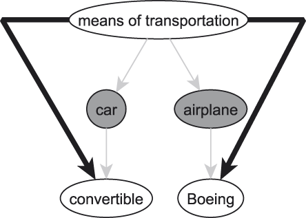
An important way in which humans organize their conceptual apparatus resides in taxonomies, a typical partial example of which is seen in Figure 1. Basic-level categories are cognitively preferenced categories by which we think about any one thing. In Figure 1, two traditionally cited examples of such categories can be found, namely car and airplane. Higher-ranked concepts are referred to as superordinate concepts / superconcepts, lower-ranked ones as subordinate concepts / subconcepts.
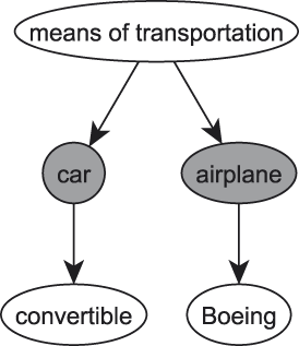
Fig. 1. Part of a taxonomy.
The seminal paper by Rosch et al. (Reference Rosch, Mervis, Gray, Johnson and Boyes-braem1976) was the first to systematically identify a number of performance advantages for basic categories. When asked to list features, people tend to list many more features for basic categories than they do for superordinate categories. In comparison, the transition to subordinate categories causes only a minor increase (Markman & Wisniewski, Reference Markman and Wisniewski1997; Mervis & Crisafi, Reference Mervis and Crisafi1982; Rosch et al., Reference Rosch, Mervis, Gray, Johnson and Boyes-braem1976; Tversky & Hemenway, Reference Tversky and Hemenway1983, Reference Tversky and Hemenway1984). A similar thing can be said about the number of motor movements people associate with categories (Rosch et al., Reference Rosch, Mervis, Gray, Johnson and Boyes-braem1976). Pictures are more readily identified in terms of basic categories than in terms of superordinate or subordinate ones (Jolicoeur, Gluck, & Kosslyn, Reference Jolicoeur, Gluck and Kosslyn1984; Lin & Murphy, Reference Lin and Murphy1997; Murphy & Brownell, Reference Murphy and Brownell1985; Murphy & Smith, Reference Murphy and Smith1982; Rosch et al., Reference Rosch, Mervis, Gray, Johnson and Boyes-braem1976; Tanaka & Taylor, Reference Tanaka and Taylor1991). Basic categories are overwhelmingly preferred in free naming (Cruse, Reference Cruse1977; Lin & Murphy, Reference Lin and Murphy1997; Morris & Murphy, Reference Morris and Murphy1990; Rosch et al., Reference Rosch, Mervis, Gray, Johnson and Boyes-braem1976; Tanaka & Taylor, Reference Tanaka and Taylor1991; Tversky & Hemenway, Reference Tversky and Hemenway1983), are more frequently used in text (Wisniewski & Murphy, Reference Wisniewski and Murphy1989), and are the first acquired by children (Anglin, Reference Anglin1977; Tanaka & Taylor, Reference Tanaka and Taylor1991).
In face of the evidence for a preferential level of conceptual representation, the question arises of what psychological aspects of the concepts account for their preference. Considerations of parsimony suggest that it is the conceptual structure that is primary. In that vein, the most widespread explanation for the preference of basic-level concepts is a structural explanation, called the differentiation explanation. Our discussion of it follows that by Murphy (Reference Murphy2002), which in turn finds its roots in Murphy and Brownell (Reference Murphy and Brownell1985), Mervis and Crisafi (Reference Mervis and Crisafi1982), and Rosch et al. (Reference Rosch, Mervis, Gray, Johnson and Boyes-braem1976). In the differentiation explanation, reference is made to two properties of concepts: informativeness and distinctiveness.
Distinctiveness refers to the degree by which a category is perceived as being different from its neighbouring categories on the same level, and is thought to drop when following a downward path in a taxonomy. Informativeness refers to the amount of information we associate with a concept, and is thought to rise when following a downward path. The higher its values on both these dimensions, the more useful a concept is considered. Not surprisingly, it is concluded that basic concepts are the ones that succeed in striking the best balance between these two forces.
This paper focuses on the idea of informativeness. The reason why informativeness is deemed to be higher in lower-ranked categories is to be sought in the notion of similarity. In Figure 1, for instance, the average similarity among instances of Boeing is said to be higher than that among instances of means of transportation. This higher similarity in turn enables people to predict more properties from knowing that something is a Boeing than from knowing that something can be classified as a means of transportation.
The goal underlying the current paper is inspired by this notion of informativeness. It is our objective to look at informativeness from a corpus linguistic angle. In contrast with the bulk of the studies done in psychology, a corpus offers a way to look at the usage of existing concepts (as opposed to artificial stimuli) in a natural (as opposed to a laboratory) setting, in which sense this study is indebted to Geeraerts et al. (Reference Geeraerts, Grondelaers and Bakema1994). In that study, a corpus linguistic approach is taken to study different kinds of variation in the lexical field of clothing. These variation effects concern the semasiological as well as the onomasiological level. The pair onomasiology/semasiology is generally regarded as identifying two different perspectives for studying the relationship between words and their semantic values. The semasiological perspective takes its starting point in the word as a form, and describes what semantic values the word may receive. The onomasiological perspective takes its starting point on the level of semantic values, and describes how a particular semantic value may be variously expressed by means of different words. In the same spirit, this paper looks at variation from a corpus linguistic angle, and more specifically at variation on the semasiological level. The main difference with Geeraerts et al. (Reference Geeraerts, Grondelaers and Bakema1994) lies in the way the study is carried out. Where the major novelty of the work of Geeraerts et al. (Reference Geeraerts, Grondelaers and Bakema1994) lies in the use of extralinguistic data,Footnote 1 the present study tries to complement that approach by maximally making use of the linguistic context we dispose of, in casu by utilizing vector space models (Agirre & Edmonds, Reference Agirre and Edmonds2006).
The working hypothesis under scrutiny can be arrived at by starting at informativeness and performing a terminological translation of the involved psychological concepts. Instances of concepts can be translated as occurrences in a corpus. Similarity between instances can be calculated by making use of token-based vector space models (Sagi et al., Reference Sagi, Kaufmann and Clark2009). By representing individual corpus occurrences as vectors in a multidimensional space an average similarity can be calculated representing the internal similarity of the concept.
We can compare the internal similarities of concepts at different levels, i.e., we can confront superordinate and basic levels (cf. Figure 2) and basic and subordinate levels (cf. Figure 3).Footnote 2 As such, the research question poses itself: Can we observe an increase in the internal similarities when we compare a higher-ranked level with a lower-ranked one? This question can be seen as the corpus linguistic counterpart of the reasoning behind the psychological notion of informativeness.
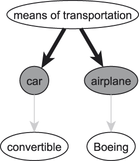
Fig. 2. Superordinate- vs. basic-level comparisons.
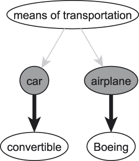
Fig. 3. Basic- vs. subordinate-level comparisons.
3. Materials
Data are assembled on the basis of the Leuvens Nieuws Corpus, which consists of a collection of six major newspapers from the Dutch-speaking part of Belgium. It holds data for Het Belang van Limburg, De Morgen, De Standaard, De Tijd, Het Nieuwsblad, and Het Laatste Nieuws for the period 1999−2005, totalling roughly 1.3 billion words. The corpus has been syntactically parsed by the Alpino parser (Bouma, Van Noord, & Malouf, Reference Bouma, Van Noord, Malouf, Daelemans, Sima’an, Veenstra and Zavrel2001).
The concepts we select are to be situated either in the semantic domain of dier (animal) or that of vervoermiddel (means of transportation). Reasons are that both of these domains are heavily studied in research on concept taxonomies, and that taken together they provide us with both natural and artefact categories. All of the selected concepts appear at least twenty times in the corpus. They either have an entry in the dictionary (den Boon & Geeraerts, Reference Boon and Geeraerts2005) or in the Dutch part of the Internet encyclopaedia Wikipedia.Footnote 3
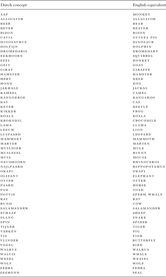
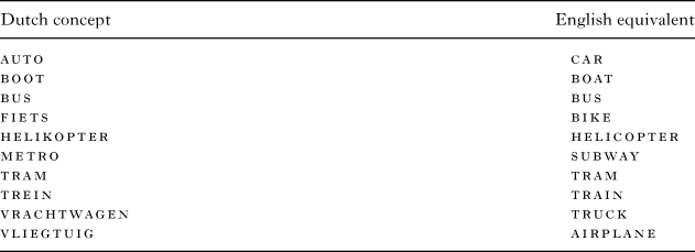
First, we collect a good deal of basic-level concepts. In spite of the number of publications concerning basic-level research, we do not dispose of readily made extensive lists giving us an overview of actual basic concepts. So, in order to steer clear as much as possible of borderline cases, our selection is closely in keeping with Rosch et al. (Reference Rosch, Mervis, Gray, Johnson and Boyes-braem1976) and with the observation by Berlin, Breedlove, and Raven (Reference Berlin, Breedlove and Raven1973) that basic concepts are usually named by primary, unanalyzable lexemes (for instance rat), which in turn often give rise to the formation of secondary lexemes as names for related subordinate concepts (for instance brown rat). The resulting collection can be found in Table A.1 (for dier) and Table A.2 (for vervoermiddel).
For each of these basic concepts we gather as many subordinate concepts as we can find. Lastly, we add as many superordinate concepts as our corpus provides us with. This gives us the counts from Table 1.
table 1. Number of concepts

Since we are interested in fixed senses, we would like to reduce the disturbing influence of polysemy. When dealing with Opel as a subconcept of auto for instance, we wish to exclude those occurrences that refer to the factory rather than to the car itself. By making use of the syntactic annotations in our corpus we are able to filter out patterns like the one just mentioned. An example of such an approach can be seen in examples (1) and (2). In example (1) Opel is used in its car meaning, while example (2) exemplifies the factory meaning. Excluding cases in which singular Opel is not preceded by any kind of determiner allows us to avoid a good deal of references to the factory.
(1) Yesterday I bought an Opel.
(2) Opel decided to close down its plant.
The number of concept occurrences we end up with can be read from Table 2.Footnote 4
table 2. Number of concept instances

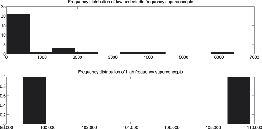
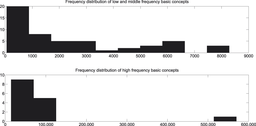
In Figures 4, 5, and 6 the frequency distributions of each of the levels can be consulted. Figure 4 takes into account the superconcepts, Figure 5 looks at the basic concepts, and Figure 6 at the subconcepts. For reasons of readability each of them distinguishes between low-, middle-, and high-frequency concepts.

Fig. 4. Frequency distribution of superconcepts.

Fig. 5. Frequency distribution of basic concepts.

Fig. 6. Frequency distribution of subconcepts.
4. Methods
To compute the internal similarity measure of our different concepts we perform the following procedure, for which we turn to Sagi et al. (Reference Sagi, Kaufmann and Clark2009) for inspiration.
1. calculate a co-occurrence matrix of ‘content-bearing’ words;
2. for each concept:
a. for each occurrence:
i. select a set of neighbouring context words;
ii. replace each context word by the corresponding vector found in the pre-computed matrix of step 1;
iii. add the vectors for each context word together to get the context vector.
b. calculate a centroid for these context vectors.
c. calculate the similarities of the context vectors to the centroid.
d. take the average of the similarities.
In Sections 4.1 and 4.2, details are provided regarding the different steps of the algorithm. We first zoom in on step 2., the major part of the algorithm. In relation to this step we should note that in order to enhance the sensitivity of our statistical tests a context vector and corresponding similarity are calculated for every occurrence we dispose of. Subsequently, details are given concerning the construction of the co-occurrence matrix of step 1.
4.1. context vectors
In this section we go through the different substeps of step 2 to arrive at the internal cohesion metric of a concept. For each occurrence of a concept a context vector is calculated. In example (3), which is a translation of a fragment we encounter in our corpus, we witness the selection of context words as outlined in step 2.a.i. For our study we select ten words to both sides of the concept occurrence. Typically, we try to avoid selecting words that are not very informative about the semantics of the context. In order to achieve this we make use of a list of stop words.
(3) When people buy a new car differentcriteria are taken into account. Among them we findcomfort, performance, price, maintenance and safety. An Opeltends to scorehigh on these criteria. Although it isn’t as expensive as its GermancompetitorsAudi, BMW and Mercedes, the car is seen as a reliable solution.
Taking into account a form of stemmingFootnote 5 of the context words gives us context vectors such as the ones seen in Table 3: the vector named Opel_1 is a partial representation for the context vector we would get for the Opel occurrence in example (3).
table 3. Example context vectors

An immediate weakness emerges from Table 3: this way of constructing context vectors is not able to capture non-literal meaning overlap. If a second occurrence Opel_2 contains the word costly, this overlap in meaning with Opel_1 is not picked up. To alleviate this important problem we conduct step 2.a.ii of the algorithm. Instead of working with the context words as we find them, called first order co-occurrences, we make use of second order co-occurrences. Applied to our example we will not work with expensive and costly directly, but instead take advantage of the co-occurrences we can in turn find for these words in our corpus. As Table 4 shows, this way of constructing context vectors does enable us to detect some similarity between Opel_1 and Opel_2 in spite of the identified problem of data sparsity. Details concerning the way this co-occurrence matrix is built up can be found in Section 4.2.
table 4. Example co-occurrence matrix

These second order co-occurrence vectors are added as indicated in step 2.a.iii, which gives us a full-blown context vector.
Having done this for all the occurrences of our concept, the next step, 2.b, consists of calculating a centroid vector for the concept. Given a set S of context vectors, the centroid C is defined as
which is the vector we obtain by averaging the weights of the context vectors v for the concept.
Steps 2.c and 2.d tell us to compute the cosine similarity of each context vector with the centroid and take the average of these similarities. Following this procedure we arrive at an internal cohesion measure.
4.2. co-occurrence matrix
The construction of a co-occurrence matrix takes its inspiration from Peirsman (Reference Peirsman2010). We too exploit the syntactic annotations our corpus disposes of and build a syntax-based space. Information about eight frequent dependency relations for a target word are taken into account:
1. subject of verb v
2. object of verb v
3. prepositional complement of verb v introduced by proposition p
4. the head of an adverbial prepositional phrase to verb v introduced by preposition p
5. modified by adjective a
6. postmodified by a prepositional phrase with head n, introduced by preposition p
7. modified by an apposition with head n, or
8. coordinated with head n
As the reader will notice, these features only work for nouns. For reasons of feasibility of computation we decided to include only nouns so as not to increase the dimensionality of our syntactic feature space too much. For our example (3) this means our algorithm only takes into account nouns, and more specifically only those nouns having an entrance in our co-occurrence matrix.
Having collected the total set of 3-tuples (target word, syntactic feature, frequency) in our corpus, some filtering is applied. Tuples containing stop words from a predetermined list are removed. Tuples with a frequency of 1 are also thrown away. A positive pointwise mutual information weighting scheme (Turney & Pantel, Reference Turney and Pantel2010) is applied. That leaves us with a matrix consisting of 52,897 target words over 102,005 dimensions.
5. Results
In a first rudimentary step we become acquainted with the behaviour of the taxonomy as a whole. Each and every relation stemming from the total collection of superordinate−basic and basic−subordinate concept pairs is taken into account (cf. Figure 7). In other words, we want to know something about the probability of finding a relation that adheres to our working hypothesis when we would pick one at random from the taxonomy.
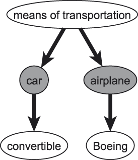
Fig. 7. Amalgam of superordinate- vs. basic- and basic- vs. subordinate-level comparisons.
To this end we use a series of t-tests to compare the internal similarities of the concepts of each couple found in the taxonomy. A total of 1,545 t-tests were conducted. The Bonferroni correction is applied to this family of statistical tests to counteract the problem of making multiple comparisons.
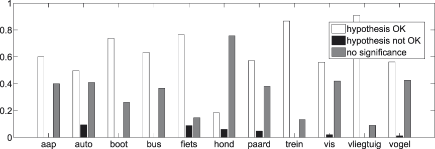
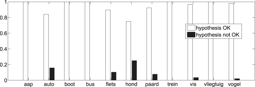
Figure 8 summarizes the outcome of this procedure. The white part indicates the proportion of comparisons in which the internal similarity of a concept stemming from a higher-ranked level is significantly (α = 3.24e-05) smaller than that of a concept beneath it: these are the comparisons that adhere to the hypothesis. In black we have the opposite situation. The grey part indicates the proportion of comparisons for which we cannot statistically assess the direction in which the comparison turns out. Figure 9 informs about the division when only significant comparisons are taken into account (the white and black parts in Figure 8), which provides us with a clear picture of the balance between successes (again in white) and failures (again in black).
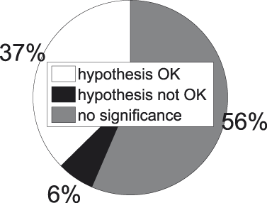
Fig. 8. t-tests for all concept pairs.
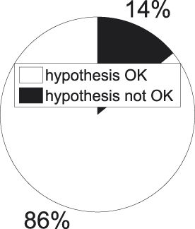
Fig. 9. t-tests for all concept pairs − significant results.
A first observation we can make with regard to Figures 8 and 9 is the high percentage of insignificant cases, i.e., cases where we do not dispose of enough evidence to statistically assess whether our hypothesis succeeds or fails.Footnote 6 The same observation recurs throughout the presentation of our results and is probably due to a combination of factors. In the first place, there is the low frequency of the majority of the subordinate concepts in our corpus (cf. Figure 6). And though each of them individually does not enter in a lot of comparisons, together they appear in a great deal of comparisons, since there are so many of them (cf. Table 1). In the second place, there is, again, the low frequency of the bulk of the superordinate concepts in our corpus (cf. Figure 4). And though there are not many of them (cf. Table 1), each of them enters into quite a number of comparisons too. Last but not least there is the Bonferroni correction, which places very stringent demands on the data.
A second observation to make is the high success rate among those cases where statistical significance is attained, especially visible in Figure 9. When a random concept pair from the collection exemplified in Figure 7 is picked, odds are we end up with one that adheres to our hypothesis, i.e., where the internal similarity of the higher-ranked concept is smaller than that of the lower-ranked one.
In a second, far more important and refined, step we discriminate between the different levels. We want to find out how the odds found in Figures 8 and 9 change when we add knowledge about the levels the concepts in the chosen concept pair stem from. In a bottom-up fashion we first look at the concept pair collection illustrated by Figure 3. Again we perform a series of t-tests, one t-test per concept pair found. In order to be able to accumulate the individual tests we again subject them to the Bonferroni correction. In total, 1,260 t-tests were performed (α = 3.97e-05). By analogy with the distinction between Figures 8 and 9, Figures 10 and 11 show the results.
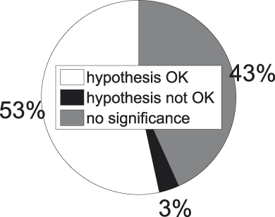
Fig. 10. t-tests for basic−subordinate concept pairs.
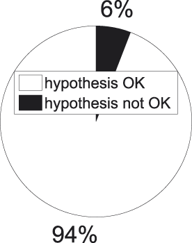
Fig. 11. t-tests for basic−subordinate concept pairs − significant results.
As both figures demonstrate, our hypothesis seems to work well when basic concepts are compared to subordinate-level concepts. In 94% of the significant cases of basic versus subordinate categories our hypothesis points out the right direction. We can also draw up a formal test to arrive at this finding. To this end we collected all concept pairs corresponding to a significant t-test and annotated them with a ‘1’ in the case of hypothesis success, and with a ‘0’ in the case of hypothesis failure. Next we take a sample that complies with the independence of sample observations, which means we see to it that a concept is selected at most once. On this sample we perform a one-tailed binomial test, resulting in a significant finding (p = 3.64e-12).
It may also prove valuable to look at the categories themselves to detect possible individual deviations. We repeat the procedure used in producing Figures 8 to 11 for those basic concepts that are involved in at least twenty t-test comparisons with subordinate concepts.Footnote 7 The exact number of comparisons per basic concept can be found in Table 5. Results are shown in Figures 12 and 13.
table 5. Number of t-test comparisons per basic concept
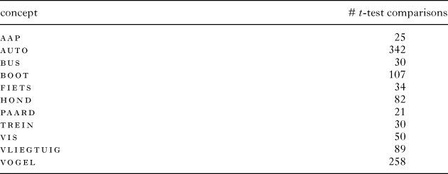

Fig. 12. t-tests per basic concept.

Fig. 13. t-tests per basic concept − significant results.
The most important thing to note about Figures 12 and 13 is their high level of consent with Figures 10 and 11. None of the basic concepts are in flat contradiction with the tendencies depicted in Figures 10 and 11. This, of course, strengthens the faith we have in the generality of the findings we make with regard to the basic−subordinate distinction. This consent does not, however, imply the total absence of variation between the categories.
We repeated the same procedure for the superordinate−basic concept pair collection, illustrated by Figure 2. In total, 285 t-tests were performed (α = 0.00018). Results are shown in Figures 14 and 15.
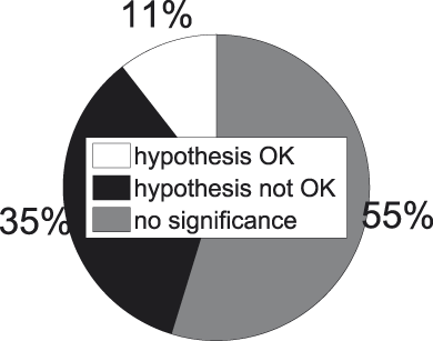
Fig. 14. t-tests for superordinate−basic concept pairs.
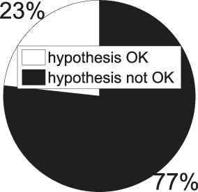
Fig. 15 t-tests for superordinate−basic concept pairs − significant results.
Things are looking less bright for our working hypothesis in this part of the taxonomy. In 77 % of the significant t-tests superordinate categories turn out to possess a higher internal similarity than the related basic concept, contradicting the hypothesis that internal similarity should drop when we move downwards in the taxonomy. A binomial test set up in the aforementioned way confirms this observation formally (p = .0013). We also see how the amalgam analysis of Figures 8 and 9 neatly conceals the failure of the working hypothesis we encounter at this stage.
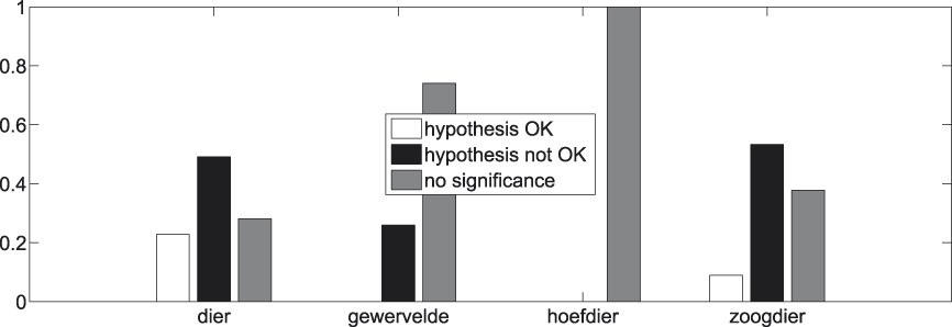
Again we have a look at the individual superordinate concepts that are involved in at least twenty t-test comparisons with basic concepts. The exact number of comparisons per superordinate concept can be found in Table 6. Results are shown in Figures 16 and17.
table 6. Number of t-test comparisons per superordinate concept


Fig. 16. t-tests per superordinate concept.
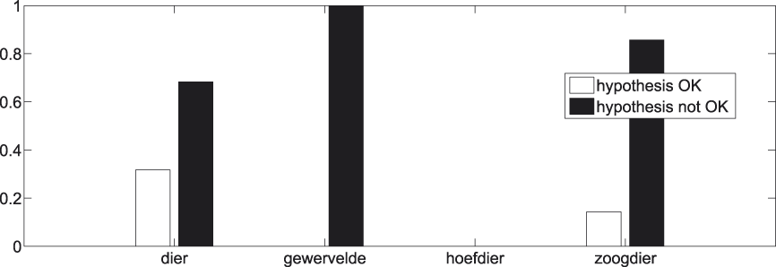
Fig. 17. t-tests per superordinate concept − significant results.
A remark similar to the one made with regard to Figures 12 and 13 can be repeated here. By and large there are no individual cases which clearly go against the tendency set out in Figures 14 and 15.Footnote 8 Again, this strengthens the faith we have in the generality of our findings pertaining to the superordinate−basic distinction.
6 Discussion
As shown earlier, our study takes its starting point in the psychological notion of informativeness and the prediction it makes about hierarchically related concepts. Lower ranked concepts are said to have a higher informativeness score because on average their members resemble each other more than those of their higher ranked competitors do. Intuitively this claim seems very plausible. We can safely assume two randomly chosen Ferraris will on average be judged more similar than two randomly chosen cars. After all, concepts are meant to capture some form of similarity between their members, so that the idea of having an inclusion relationship between two concepts seems to imply a higher internal similarity on the part of the subconcept.Footnote 9
Our own investigation deviates from the informativeness claim in some important ways. A first deviation from the background against which the informativeness hypothesis is formulated resides in the nature of the features we use, and determines how we should interpret our internal similarity score. While the informativeness hypothesis looks at properties which are thought to constitute the concept, this paper is based on distributive behaviour obtained by vector space models. Vector space models operate by the distributional hypothesis: words that occur in similar contexts tend to have similar meanings (Deerwester, Dumais, Furnas, Landauer, & Harshman, Reference Deerwester, Dumais, Furnas, Landauer and Harshman1990; Firth, Reference Firth and Firth1957; Harris, Reference Harris1954). If one takes this claim seriously, the study of distributional patterns can teach us something about the semantics of concepts. Since we try to compare the semantic similarity of the various contexts of use of a concept, the similarities we obtain can be seen as modelling the degree to which different concepts show a kind of homogeneity in the way they are used. Concepts scoring high on our internal similarity scale can be thought of as more predictive of the contexts in which they are used than concepts associated with lower scores.
A second deviation lies in the way the extension of the concept is being determined. Whereas the informativeness hypothesis focuses on the extension of concepts in a decontextualized way, our corpus linguistic approach shifts the focus to concepts as they are actually being used. From the point of view of informativeness, each and every referent which can be categorized as car is taken into account in the calculation of car’s informativeness score, while our study only considers those referents that are actually being named ‘car’. In other words, we require an act of categorization. This holds the possibility that some of the referents taken into account by the informativeness criterion are ignored by our method. Another difference which can arise is shifts in the relative weight of importance of groups of members. Various referents may be accompanied by different naming preferences (Geeraerts et al., Reference Geeraerts, Grondelaers and Bakema1994), which can in turn provide us with a different picture of the extension of categories than the one used by the informativeness approach.
With the foregoing in mind we are now in a position to try to interpret our findings. As Figures 10, 11, 14, and 15 show, basic concepts are generally less predictive of their context of use than related superordinate or subordinate concepts. The basic−subordinate relation is as hypothesized; the superordinate−basic relation is not. In spite of its more extended denotation, a superordinate concept is used in contexts which on average are more similar to each other than those in which a related basic concept appears.
We believe the second deviation mentioned above might prove crucial in understanding these results and why they do not accurately parallel those of the informativeness claim. In his research on discourse differences between the three psychologically discerned levels, Cruse (Reference Cruse1977) notes that, unless they are specifically called for, reference is not usually made through superordinate or subordinate concepts. He finds that, in most contexts, basic concepts constitute the more neutral specification, whereas the other two levels often produce a marked effect. Subordinate and superordinate concepts seem to require certain circumstances in order to be the adequate lexical choice. Subordinate concepts are often used in discourse when the additional information they provide vis-à-vis their basic-level concept is particularly relevant (Cruse, Reference Cruse1977; Murphy & Brownell, Reference Murphy and Brownell1985). Their use is common, too, when there is a domain that contains many members of a basic category that need to be distinguished (Murphy, Reference Murphy2002). Superordinate concepts in turn can highlight the abstract, functional properties they dispose of (Murphy, Reference Murphy2002; Rosch et al., Reference Rosch, Mervis, Gray, Johnson and Boyes-braem1976; Tversky & Hemenway, Reference Tversky and Hemenway1984), and are often used to refer to a collection of a number of items belonging to different basic-level concepts (Markman, Reference Markman1985; Murphy, Reference Murphy2002; Wisniewski, Imai, & Casey, Reference Wisniewski, Imai and Casey1996; Wisniewski & Murphy, Reference Wisniewski and Murphy1989).
If it is the case that basic concepts often constitute a ‘default’ choice in discourse, and if it is true that the use of concepts belonging to the other two levels calls for some more ‘specific’ circumstances, then the extension (as talked about in the second deviation above) of superordinate and subordinate concepts could be more restricted than that of related basic concepts. In that case it would not seem too far-fetched to expect our internal similarity measure to turn out higher in the case of a subordinate or superordinate concept than in the case of a related basic concept. That being said, we would like to stress the direction of causality. Since our research takes a semasiological stand our results cannot sensibly be used to prove the truth of the above claims concerning lexical choice in discourse. In the case of their truth, however, our results could sensibly be explained by them, as we have tried to do, and not vice versa.
Yet this does not necessarily entail the total and utter absence of taxonomical denotation in the story of our internal similarity measure. Figures 10, 11, 14, and 15 suggest a stronger tendency in the case of the basic−subordinate relations than in case of the superordinate−basic relations. We therefore consider it interesting to confront superordinate and subordinate concepts too (cf. Figure 18).

Fig. 18. Superordinate- vs. subordinate-level comparisons.
In total, 3,613 t-tests were performed (α = 1.38e-05). The results are displayed in Figures 19 and 20 in a fashion reminiscent of what has been done in Section 5.
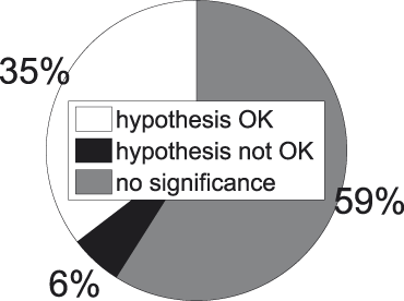
Fig. 19. t-tests for superordinate−subordinate concept pairs.
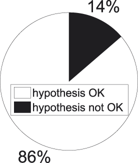
Fig. 20. t-tests for superordinate−subordinate concept pairs − significant results.
Figures 19 and 20 show that superordinate concepts are in general less predictive of their context of use than subordinate concepts. A one-tailed binomial test set up in the way demonstrated in Section 5 confirms this observation formally (p = .011). So in this case, where the basic level is not a contender, it seems to be that the much more limited denotation of subordinate concepts in comparison to related superordinate ones causes them to be more predictive of their context of use than those superordinate concepts.
In spite of these general tendencies it is important not to lose sight of the variation we encounter too. Figures 10, 11, 14, and 15 show that not all concept pairs follow the direction taken by the majority, while Figures 12, 13, 16, and 17 demonstrate that there is also variation to be found regarding the degree to which different concepts on the same level adhere to the general tendencies. In that way our findings are somewhat reminiscent of an important insight Geeraerts et al. (Reference Geeraerts, Grondelaers and Bakema1994) describe. There it is claimed that the basic-level model as a model of onomasiological salience is insufficient, since it does not capture the differences the authors found in onomasiological salience between concepts of the same taxonomical level, and since it does not predict their empirical finding that subordinate concepts can be as onomasiologically salient as their basic-level concept. The suggestion the authors made is that the basic-level model only captures a general tendency, and merely that. A more precise account of onomasiological salience needs to be prepared to look at individual categories at any level of the hierarchy and should expect observations going beyond the general predictions of the basic-level model. That same idea can be incorporated here in relation to the internal similarity score. Whereas there does indeed seem to be a general pattern for basic-level concepts to dispose of lower internal cohesion than related concepts from other levels, the results nonetheless deviate from this tendency for a number of category pairs. Looking at concepts as they are actually being used seems to ask us to broaden our horizon, by forcing us to drop a strictly logical perspective on taxonomies of concepts, and to be prepared to have a look at concepts individually. The patterns we find are real, but they are not like a law of the Medes and Persians.
To sum it up, we can say that, in imitation of a group of other measures, the basic level also holds a special position with regard to the internal similarity of concepts based on their distributional behaviour: basic concepts are generally less predictive of their context of use than related superordinate or subordinate concepts. However, we should not make this observation absolute. Corpus-specific characteristics can allow for individual deviations from this pattern. Secondly, we cannot forget about taxonomical denotation. Although it has not as decisive a role to play as in the informativeness criterion, taxonomical denotation nonetheless constitutes an important determinant of corpus-based internal similarity, as superordinate concepts are generally less predictive of their context of use than related subordinate concepts. Once again, though, some room should be left for individual deviations.
APPENDIX
table A.1. Basic concepts in dier (animal)

table A.2. Basic concepts in vervoermiddel (means of transportation)


