Introduction
From an agricultural perspective, knowledge regarding the factors that induce phenological patterns in pest species is crucial for proper pest control and management (Dennis et al., Reference Dennis, Kemp and Beckwith1986). Two main parameters have been used to identify and quantify phenological events: the periods of occurrence and intensity of phenology (Morellato et al., Reference Morellato, Talora, Takahasi, Bencke, Romera and Zipparro2000; Zar, Reference Zar and Zar2010). The first represents the period when over which the phenological event is expressed. The second is not related to the period of the phenological event itself, but to how long it occurs throughout the year (Morellato et al., Reference Morellato, Talora, Takahasi, Bencke, Romera and Zipparro2000; Ting et al., Reference Ting, Hartley and Burns2008). Therefore, the intensity of phenology is a parameter positively related to the total abundance of observations throughout the year and negatively related to the duration of this phenomenon.
Latitudinal gradients represent an optimal scenario to study the way the organisms regulate their phenological patterns (either the occurrence period and/or phenological intensity) given the temporal fluctuations in climate and food availability (Garibaldi et al., Reference Garibaldi, Kitzberger and Ruggiero2011; De Frenne et al., Reference De Frenne, Graae, Rodríguez-Sánchez, Kolb, Chabrerie, Decocq, De Kort, De Schrijver, Diekmann, Eriksson, Gruwez, Hermy, Lenoir, Plue, Coomes, Verheyen and Giliam2013). In this context, the Noctuid moth pests have been identified as suitable models for these studies, as they enable comparisons to be made of the different phenological responses of the same species in different sites. Insect pests adversely impact many crop species, causing average annual economic losses of up to 18% (Oerke, Reference Oerke2006), as seen in genus Spodoptera, for instance. The genus includes 30 species, most of them having wide geographical distribution and at least 50% of these are economically significant, as they consume many of the principal crop species across the world (Pogue, Reference Pogue2002).
While information on the geographic distribution and host plants of the South American Spodoptera species is available (Pogue, Reference Pogue2002; Specht & Roque-Specht, Reference Specht and Roque-Specht2016), data regarding the duration and period of occurrence are very limited (Murúa et al., Reference Murúa, Molina-Ochoa and Coviella2006). When available, most of the documentation comes from laboratory experiments, which are usually limited to local findings, not taking into account the natural fluctuations across a wide latitudinal scale (Bavaresco et al., Reference Bavaresco, Garcia, Grützmacher, Ringenberg and Foresti2004; Zenker et al., Reference Zenker, Botton, Teston and Specht2010; Montezano et al., Reference Montezano, Specht, Sosa-Gómez, Roque-Specht and Barros2013; Almeida et al., Reference Almeida, Specht and Teston2014; Montezano et al., Reference Montezano, Specht, Sosa-Gomez, Roque-Specht, Bortolin, Fronza, Pezzi, Luz and Barros2014). Some meteorological factors, such as temperature, precipitation, and photoperiod, may be linked to insect phenology (Garibaldi et al., Reference Garibaldi, Kitzberger and Ruggiero2011). They may directly influence phenology when they affect the pest itself or indirectly when they affect the availability and quality of its food source (Porter et al., Reference Porter, Parry and Carter1991; Cammell & Knight, Reference Cammell and Knight1992; Garibaldi et al., Reference Garibaldi, Kitzberger and Ruggiero2011), both in the natural and agricultural habitats (Altermatt, Reference Altermatt2010). On the other hand, food availability may be a predominant factor when vast quantities of the food sources previously available through, for example, monoculture, become limited due to changes in cropping and harvesting patterns (Cocu et al., Reference Cocu, Harrington, Rounsevell, Worner and Hulle2005).
The annual population dynamics exhibited by the Spodoptera species along the 29° latitudinal gradient in Brazil are used in this study to test the following null hypotheses: (1) as these species are abundant in the agricultural ecosystems and can be recorded throughout the year, they all reveal similar phenological patterns along the latitudinal gradient; (2) meteorological factors and host plant availability similarly influence the period of occurrence and phenology intensity of all armyworm species.
Materials and methods
Sampling
Spodoptera adults were sampled from June 2015 to May 2016, in 13 locations, positioned along the latitudinal gradient of −2° to −31°, covering four Brazilian biomes (table 1) (IBGE, 2004). At each location, a Pennsylvania type light trap was installed (Frost, Reference Frost1957) provided with a BL T8 15W Black Light fluorescent lamp, having wavelengths from 290 to 450 nm, and a maximum of about 340 nm. The traps set at about 3.0 m height above the ground were operated for around 12 h, from twilight until dawn, for five nights per new moon cycle (Yela & Holyoak, Reference Yela and Holyoak1997), for 12 months, or 60 nights of sample collection per trap.
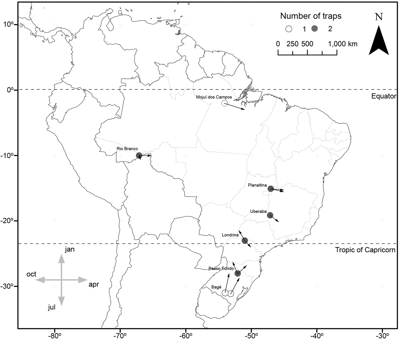
Table 1. Sampling sites and abundance of Spodoptera spp. sampled in a latitudinal gradient in Brazil.
Numbers beside localities discriminate trap sites.
TS, temperature seasonality (standard deviation × 100); PS, precipitation seasonality (coefficient of variation). Climatic data extracted from Hijmans et al. (Reference Hijmans, Cameron, Parra, Jones and Jarvis2005).
However, the light traps could vary in efficiency as they were affected by abiotic factors, including wind velocity, temperature, and, principally, the lunar luminosity (Yela & Holyoak, Reference Yela and Holyoak1997). To minimize this sampling effect, only three nights for each trap during the new moon cycle were considered, selecting the three samples which showed the largest number of individuals collected. The insects collected daily were sorted, identified (Pogue, Reference Pogue2002), and prepared in the laboratory. Voucher specimens were deposited in the ‘Coleção Entomológica da Embrapa Cerrados’ and Coleção Entomológica Pe. Jesus Santiago Moure, Departamento de Zoologia, Universidade Federal do Paraná, Brazil.
Predictor variables
With the objective of identifying the predictive power of the factors responsible for the phenological patterns exhibited by the species, the data were collected on the availability of food surrounding (e.g. host plant area) each trap and climatic region. Food availability was estimated using buffer zones with two different scales of 100 and 400 m. Employing the Google Earth Pro (2017) software, the cultivated and uncultivated parts of the regions within each buffer zone were quantified.
The cultivars were distinguished in terms of the vegetative species and cultivation period (from planting time to harvest), while the uncultivated areas were considered perennial. Therefore, the size of the areas was multiplied by the number of days that the plants were present, thus quantifying the food availability for the Spodoptera populations (Supplementary table S1). Most of the sampling sites had a predominantly agricultural landscape supporting the annual soybean (Glycine max (L.) Merril) and maize (Zea mays L.) crops, each cultivated for 3–4 months. Secondarily, there were other species such as Sorghum bicolor ((L.) Moench) and several species of pasture crops including Andropogon spp., Panicum spp., Brachiaria decumbens Stapf., Melinis multiflora (P. Beauv.), Pennisetum purpureum (Persoon), Avena spp., and Lolium multiflorum (Lam.) (Montezano et al., Reference Montezano, Specht, Sosa-Gómez, Roque-Specht and Barros2013; Specht & Roque-Specht, Reference Specht and Roque-Specht2016).
Furthermore, latitude and climate seasonality were also used as predictors of Spodoptera phenology. The climate metrics were represented by annual temperature seasonality and annual precipitation seasonality. The first represents the amount of temperature variation over a given year based on the standard deviation (SD) (variation) of monthly temperature averages, while the second is a measure of the variation in monthly precipitation totals over the course of the year. This index is the ratio of the SD of the monthly total precipitation to the mean monthly total precipitation (also known as the coefficient of variation) and is expressed as a percentage (O'Donnell & Ignizio, Reference O'Donnell and Ignizio2012). These variables are available in WorldClim database (Hijmans et al., Reference Hijmans, Cameron, Parra, Jones and Jarvis2005).
Statistical analyses
Circular statistical tools are recommended to identify and discern phenological patterns of different species (Morellato et al., Reference Morellato, Talora, Takahasi, Bencke, Romera and Zipparro2000; Brito et al., Reference Brito, Ribeiro, Raniero, Hasui, Ramos and Arab2014). These tools transform value categories into angles ranging from 0 to 360° in a circle, whose ‘0’ value is arbitrarily established (Zar, Reference Zar and Zar2010). Hence, the occurrence dates of a phenological observation are transformed to an angle proportional to the circularity of the 365 days in a year (e.g. n° days × 360/365). The phenological parameters estimated in this study included (a) period of occurrence and (b) intensity of phenology. These indices were identified, based on the non-uniformity of the abundance distributions over time, which implied validation of the phenological variation present. Rao's Spacing test was employed to accomplish this for the data that did not show unimodal distribution (Bergin, Reference Bergin1991; Ribeiro et al., Reference Ribeiro, Prado, Brown and Freitas2010), as is evident. All the samples lacking significant values for the Rao's Spacing test were excluded from further analyses. After rejecting the hypothesis of uniform yearly abundances, the mean angle (μ) can be used to represent the concentration of abundances for a specified period of the year. This means that if the higher species abundance is related to a specific part of the year, it can be understood to be the period of occurrence exhibited by a particular species. Besides, once the mean angle is used to determine the period of occurrence, the SD of the mean angle can be calculated to represent the intensity of this phenomena (Morellato et al., Reference Morellato, Talora, Takahasi, Bencke, Romera and Zipparro2000; Ting et al., Reference Ting, Hartley and Burns2008; Brito et al., Reference Brito, Ribeiro, Raniero, Hasui, Ramos and Arab2014). Therefore, SD determines the degree to which Spodoptera species are available throughout the year.
Two analyses were performed to test for the predictive factors responsible for the variations observed in the period of occurrence of the species. The first verified whether the average angle that represents the period of occurrence of the species is associated with the latitude at which each trap had been set up. As these variables are circular and linear, respectively, a circular–circular correlation test was used. The second analysis tested whether the period of occurrence for each species was synchronous with the time when the main crops (e.g. soybean, corn, wheat, sorghum, and pastures) were present in each site. The average angle of each crop available at the location of each trap (100 and 400 m scales) was calculated through its own circular average, assessed between the angles of the months during which the crops were present. In this analysis, the V test available in the Oriana 4.0 program was used (Kovach, Reference Kovach2011).
Likewise, we tested whether the same parameters described above influenced the intensity of phenology of the different Spodoptera species. In this analysis, the SD of the mean angle for each species, in each sample, drawn from the circular analyses was used as a surrogate of phenological intensity (Morellato et al., Reference Morellato, Talora, Takahasi, Bencke, Romera and Zipparro2000). But because this is a linear variable, it could be determined using linear regression models. The variables chosen as predictors included the period of occurrence of the soybean and maize crops (in days), seasonality of temperature and precipitation, as well as latitude. In addition, a null model was added using the random values, resulting in a total of six models for each species, each one having a single predictor variable. For each species, the best model produced for the intensity of phenology was chosen based on the Corrected Akaike Information Criterion (AICc) (Burnham & Anderson, Reference Burnham and Anderson2004; Burnham et al., Reference Burnham, Anderson and Huyvaert2011).
The weights drawn from the AICc varies from 0 to 1, in which the closer the value is to 1 the greater the predictive power yielded by the model. The support provided by alternative models is determined by the differences in the AICc values, in which a difference value of below 2 implies equally plausible models (Burnham & Anderson, Reference Burnham and Anderson2004; Burnham et al., Reference Burnham, Anderson and Huyvaert2011). As all the models are classified according to this value, the null model acts as a reference, enabling the identification and quantification of the variables having the best predictive power. Circular statistics, linear models, and comparisons of AICc were done using CircStats (Agostinelli, Reference Agostinelli2012) and bbmle (Bolker, Reference Bolker2017) package in R environment (R Core Team, 2015).
Results
Along the entire latitudinal gradient, a total of 5277 Spodoptera adults were collected from all the traps, with an average of 11 individuals captured per trap/night. Low numbers and/or presence in a few localities made it impossible to assess the phenological patterns of S. marima (Schaus, 1904), S. eridania (Stoll, 1782), S. dolichos (Fabricius, 1794), and S. androgea (Stoll, 1782). In most of the samples, these species revealed abundances in non-uniform distributions through the year, and their non-significant values were normally related to the occasional poor numbers of specimens captured. Hence, the results for S. albula, S. cosmioides, and S. frugiperda only are reported (table 2).
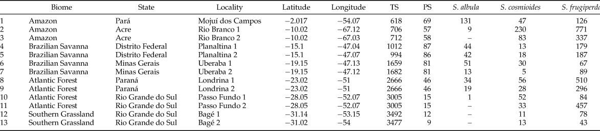
Table 2. Descriptive statistics derived from circular analysis of the abundance of Spodoptera collected with light traps, in the three most abundant nights on each new moon per locality.

N, moths abundance; μ, mean circular vector; CSD, circular standard deviation; U, Rao's Spacing test.
**<0.01 Significant values.
Period of occurrence
In the cases of S. albula and S. cosmioides, the occurrence periods showed significant correlation with latitude (R 2 = 0.72, P < 0.05; R 2 = 0.64, P < 0.05). Therefore, at the lower latitudes, S. albula was found between February and April. But as the latitudes increases, the period of occurrence of this species extends from April to June (fig. 1). Spodoptera cosmioides, at the lower latitudes, occur mostly between April to July. However, with the increase in latitude, this period of occurrence shifts from December to May (fig. 2). On the other hand, S. frugiperda exhibited no relationship between the period of occurrence and latitude (R 2 −0.2, P > 0.05) (fig. 3). Additionally, the mean occurrence of Spodoptera species corresponded to the time span when the main host plant species were grown throughout the year. Soybean and corn, in particular, showed the greatest correlation with their period of occurrence. From among all the crop species cultivated, S. albula showed the least number of correlations (30% of the cultivated species; 50% of the sampled localities), followed by S. cosmioides (34% of the cultivated species; 73% of the sampled localities) and finally S. frugiperda (75% of the cultivated species; 83% of the sampling sites) (Supplementary table S2).
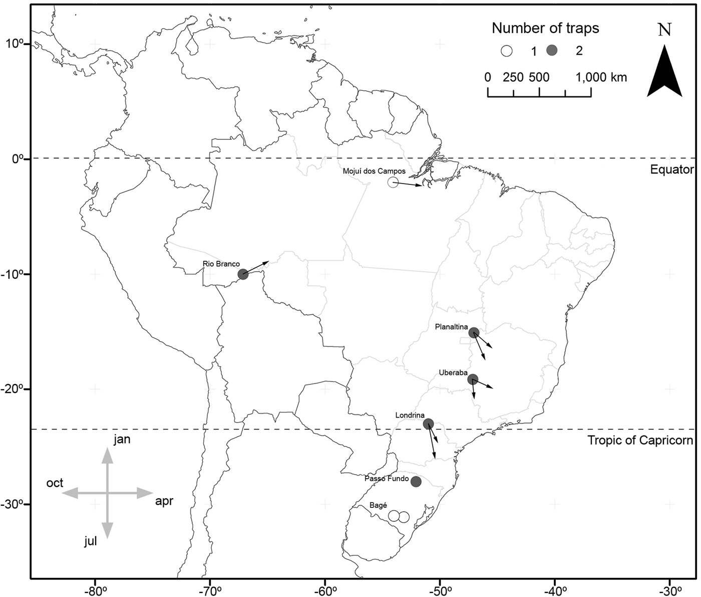
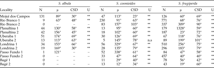
Fig. 1. Map illustrating the geographical distribution of sample sites, representing one (white) or two (gray) traps each. Vectors (arrows) point mean occurrence period, while its length represents the phenology intensity exhibited by Spodoptera albula.

Fig. 2. Map illustrating the geographical distribution of sample sites, representing one (white) or two (gray) traps each. Vectors (arrows) point mean occurrence period, while its length represents the phenology intensity exhibited by Spodoptera cosmioides.

Fig. 3. Map illustrating the geographical distribution of sample sites, representing one (white) or two (gray) traps each. Vectors (arrows) point mean occurrence period, while its length represents the phenology intensity exhibited by Spodoptera frugiperda.
Intensity of phenology
The intensity of phenology was predicted in a similar manner, using the two scales analyzed (100 and 400 m). However, in this case, the null model revealed the best predictive power for the intensity of phenology for S. albula and S. cosmioides. On the contrary, the seasonality of the precipitation and temperature predicted the higher intensity of phenology in S. frugiperda along the entire latitudinal gradient (table 3), supporting the concept that each species of Spodoptera has its own specific response to the abiotic and biotic factors.
Table 3. Variables correlated to the phenology intensity of Spodoptera species, ranked by the Corrected Akaike Information Criterion (AICc), at 400 and 100 m buffer size.
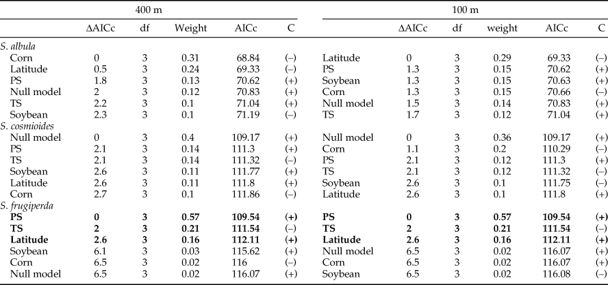
The variables in bold indicate a higher predictive power when compared with the null model. ΔAICc, differences relative to the smallest AICc value in the model set; df, degrees of freedom as associated with hypothesis testing; weight, Akaike weight; C, correlation polarity; TS, temperature seasonality (standard deviation × 100); PS, precipitation seasonality (coefficient of variation). Climatic data extracted from Hijmans et al. (Reference Hijmans, Cameron, Parra, Jones and Jarvis2005)
Discussion
Period of occurrence
In contrast to natural environments (Wolda, Reference Wolda1988; Kishimoto-Yamada & Itioka, Reference Kishimoto-Yamada and Itioka2015), only a few phenological studies related to latitude have been conducted in agricultural ecosystems (Cocu et al., Reference Cocu, Harrington, Rounsevell, Worner and Hulle2005). Usually local studies restricted to minor latitudinal gradients do not contribute understanding of the phenological plasticity of a particular species (Fielding et al., Reference Fielding, Whittaker, Butterfield and Coulson1999). Therefore, the period of occurrence for several widespread pest species remains unknown, despite such understanding being highly relevant for global food production (Régnière & Sharov, Reference Régnière and Sharov1998; Donatelli et al., Reference Donatelli, Magarey, Bregaglio, Willocquet, Whish and Savary2017). The phenological responses of organisms can reveal variations along the entire latitudinal gradient and the factors usually linked to this phenomenon include temperature, precipitation, and photoperiod (here represented as latitude). As the latitudes move away from the tropics, greater seasonality in the temperature and photoperiod is observed, but less seasonality in precipitation (De Frenne et al., Reference De Frenne, Graae, Rodríguez-Sánchez, Kolb, Chabrerie, Decocq, De Kort, De Schrijver, Diekmann, Eriksson, Gruwez, Hermy, Lenoir, Plue, Coomes, Verheyen and Giliam2013).
These variables are most often related to the insects’ life cycles, and correspond to the periods of occurrence of S. albula and S. cosmioides. Interestingly, the periods of occurrence and variables influencing this phenological pattern are different for both these species along the entire latitudinal gradient investigated in this study. The occurrence of S. albula was observed to be delayed as the latitude increased. Pieris rapae (Linnaeus, 1758) (Gordo et al., Reference Gordo, Sanz and Lobo2010) and Cactoblastis cactorum (Berg, 1885) (Hight & Carpenter, Reference Hight and Carpenter2009) in the Northern Hemisphere exhibited similar patterns, although within a narrower latitudinal gradient. In regions where the temperature differences are well defined (e.g. Southern Brazil), insect activity is more evident during the hotter seasons (Wolda, Reference Wolda1988). However, temperature differences do not appear to significantly affect the period of occurrence for S. albula, as its occurrence in the highest latitudes corresponds with the months experiencing low temperatures.
The availability of crops also does not seem to be a determining factor for the period of occurrence for S. albula, as this coincides only with the period of cultivation of plants not utilized by the species (e.g. pasture and wheat) (Montezano et al., Reference Montezano, Specht, Sosa-Gómez, Roque-Specht and Barros2013). Curiously, S. albula revealed the highest abundance in those areas showing marked seasonality of precipitation (dry season), which is in agreement with the results of Piovesan et al., (Reference Piovesan, Specht, Carneiro, Paula-Moraes and Casagrande2017). Even in the highest latitudes, the period of occurrence of S. albula corresponds with the months experiencing low humidity. Likewise, its sister species, S. ochrea (Hampson, 1909) occurs especially in the dry ecosystems of Peru and Ecuador (Pogue & Passoa, Reference Pogue and Passoa2000; Pogue, Reference Pogue2002; Kergoat et al., Reference Kergoat, Prowell, Le Ru, Mitchell, Dumas, Clamens, Condamine and Silvain2012) suggesting an adaptation of these species to highly seasonal environments or at least when any given season experiences low precipitation rates.
By contrast, S. cosmioides, like other insects (Wolda, Reference Wolda1988), reveals an inverse period of occurrence to that of S. albula, which increases with the rise in latitude. Therefore, this species occurs in greater abundance during the hotter and wetter seasons, in places experiencing more seasonal temperatures. However, the greater synchronization between the availability of the host plant and occurrence periods of both S. cosmioides and S. frugiperda suggests that these species have developed more intrinsic relationships with the crop species in agricultural ecosystems although specific differences were identified between them. While S. cosmioides tended to be linked chiefly with the availability of soybean and corn crops, S. frugiperda was associated with many host plant species, regardless of the latitude or crop season. This indicates that these species are affected only secondarily by climatic conditions and that they are most abundant when their principal crop species are available (e.g. soybean, maize) (Thiéry et al., Reference Thiéry, Monceau and Moreau2014).
Interestingly, S. frugiperda displayed striking differences in occurrence in regions exhibiting only slight differences in latitude, similar climatic (clear-cut seasons) and agricultural conditions (same species cultivated during the same period). At present, it is still difficult to understand the population dynamics of S. frugiperda, as these variations may be linked to at least two biotypes present, known as the ‘rice-strain’ and ‘corn-strain’ (Pashley et al., Reference Pashley, Johnson and Sparks1985; Nagoshi & Meagher, Reference Nagoshi and Meagher2004). Nagoshi & Meagher (Reference Nagoshi and Meagher2004) report that both strains reveal sharp temporal variations in response to the seasonal conditions. However, it was not possible to study temporal variations among the various biotypes in the present work.
Another relevant phenomenon is the possibility that some Spodoptera species migrate along latitudinal gradients, as climate and host plant availability also changes accordingly. If such a phenomenon occurs, we would expect to find a similar population size occurring at different periods of the year, thus corroborating the patterns found for S. albula and S. cosmioides. However, it should be noted that unlike in the Northern Hemisphere (Nagoshi et al., Reference Nagoshi, Meagher and Hay-Roe2012; Reference Nagoshi, Fleischer, Meagher, Hay-Roe, Khan, Murúa, Silvie, Vergara and Westbrook2017), the central region of Brazil (covered by the savanna ecosystems) experiences extreme droughts during the winter (from May to September), thus probably isolating populations from Northern and Southern Brazil and suppressing migrant behavior. In this context, molecular studies are necessary to test this hypothesis.
Intensity of phenology
The variables of climate and food availability may also affect the intensity of the phenological pattern of the species, without actually impacting the time of their occurrence (Ting et al., Reference Ting, Hartley and Burns2008). However, in this study, S. frugiperda was the only species to reveal a variation in the phenological intensity correlated with latitude. This species occurred in greater concentrations (e.g. with stronger phenological intensity) in the higher latitudes and, therefore, exhibited higher climatic seasonality (De Frenne et al., Reference De Frenne, Graae, Rodríguez-Sánchez, Kolb, Chabrerie, Decocq, De Kort, De Schrijver, Diekmann, Eriksson, Gruwez, Hermy, Lenoir, Plue, Coomes, Verheyen and Giliam2013), but is likely to be more homogeneous at the lower latitudes where smaller temperatures are less variable (Wolda, Reference Wolda1988). Therefore, host plant availability appears to change their period of occurrence; however, the intensity or length of this period is linked to climatic factors.
These findings suggest that such dissimilarities in phenology may be related to biotic, abiotic, or both factors (Day, Reference Day1984; Eizaguirre et al., Reference Eizaguirre, López and Sans2002; Jang et al., Reference Jang, Siderhurst, Conant and Siderhurst2009; Garibaldi et al., Reference Garibaldi, Kitzberger and Ruggiero2011; Ortega-López et al., Reference Ortega-López, Amo-Salas, Ortiz-Barredo and Díez-Navajas2014; Doherty et al., Reference Doherty, Guay and Cloutier2017), and will depend on the pest species. Yet, there are many other factors that can also influence the moth population variation measured in this study, for instance the presence and abundance of predators, parasitoids, and pathogens (Wolda, Reference Wolda1988; Kishimoto-Yamada & Itioka, Reference Kishimoto-Yamada and Itioka2015). However, there are still many challenges to quantify these kind of variables in tropical regions, as many of these ecological relationships are still poorly documented.
Conclusions
By assessing the period of occurrence and degree of phenological intensity, this study reveals that the species studied show unique adaptive strategies for the varying conditions generated by the global latitudinal gradient. Hence, pest management techniques should also take into account the latitudinal location of the host crops. For instance, strategies employed in the management of S. albula and S. cosmioides need to focus on specific months of the year, when these species are found along different latitudinal gradients. On the other hand, the management of S. frugiperda should focus on the period when soybean, corn, wheat, sorghum, and pasture crops are grown, regardless of the time of the year, at the various latitudinal sites. Furthermore, more intense monitoring is necessary at the higher latitudes, during the periods of higher temperatures, while uninterrupted monitoring is required at the lower latitudes, as the phenological intensity decreases. With the prospect of climate change (Peñuelas et al., Reference Peñuelas, Rutishauser and Filella2009; De Frenne et al., Reference De Frenne, Graae, Rodríguez-Sánchez, Kolb, Chabrerie, Decocq, De Kort, De Schrijver, Diekmann, Eriksson, Gruwez, Hermy, Lenoir, Plue, Coomes, Verheyen and Giliam2013), a clear understanding of the phenological patterns of pest species becomes central to their management, as they will assist in the prediction of pest incidence in different geographical regions in the future.
Supplementary material
The supplementary material for this article can be found at https://doi.org/10.1017/S0007485318000822
Acknowledgements
To Maicon Coradini, José Augusto Teston, Murilo Fazolin, Felipe de Oliveira Mateus, Adriano Queiroz de Mesquita, Vander Célio de Matos Claudino, Américo Iorio Ciciola Júnior, Daniel Ricardo Sosa-Gómez, Oriverto Tonon, Wilson Pozenato, Paulo Roberto Valle da Silva Pereira, Rodison Natividade Sisti, Jorge Ubirajara Pinheiro Corrêa, Marco Antônio Padilha da Silva, Harry Ebert, Naylor Bastiani Perez for aiding in sampling. To Brenda Melo Moreira, Fabio Luis dos Santos, Luziany Queiroz Santos, Martha Cecilia Erazo Moreno, Sabrina Raisa dos Santos for aiding in specimen sorting and identifying. We also thank two anonymous reviewers for helpful comments on the manuscript.
Funding
To research funding from Conselho Nacional de Desenvolvimento Científico e Tecnológico (CNPq) (procs. N°. 403376/2013-0 and 302084/2017-7). To Empresa Brasileira de Pesquisa Agropecuária (EMBRAPA) (SEG MP2 n° 02.13.14.006.00.00) and to Instituto Chico Mendes (ICMBio) – Ministério do Meio Ambiente do Brasil – Authorization for scientific activities SISBIO 48218(1-3).