


1. Introduction
The geomagnetic field acts as a shield to protect us from solar wind (Tarduno Reference Tarduno2018) apart from directly influencing the atmosphere (Cnossen Reference Cnossen2014), biology and evolution of life on Earth (Erdmann et al. Reference Erdmann, Kmita, Kosicki and Kaczmarek2021). Such magnetic fields of planets and stars are known to be generated by a dynamo mechanism driven by the convection of electrically conducting fluids (Rüdiger & Hollerbach Reference Rüdiger and Hollerbach2006). In this self-sustained dynamo mechanism, the convective motion of electrically conducting fluids leads to the amplification of a small magnetic perturbation by electromagnetic induction. The induced magnetic field is then maintained against Joule dissipation by continuously converting some of the kinetic energy of the fluid to magnetic energy. A simple model of such dynamos is the Rayleigh–Bénard convection (RBC) in a plane layer between two parallel plates, heated from the bottom and cooled from the top, permeated by a magnetic field. Inclusion of global rotation in such flows can break the reflectional symmetry of the convection to induce large-scale magnetic fields (Moffatt & Dormy Reference Moffatt and Dormy2019; Tobias Reference Tobias2021). Non-magnetic rotating convection (RC) has been studied extensively using experiments (King et al. Reference King, Stellmach, Noir, Hansen and Aurnou2009; Kunnen, Geurts & Clercx Reference Kunnen, Geurts and Clercx2010; King & Aurnou Reference King and Aurnou2013; Ecke & Niemela Reference Ecke and Niemela2014; Stellmach et al. Reference Stellmach, Lischper, Julien, Vasil, Cheng, Ribeiro, King and Aurnou2014; Aurnou et al. Reference Aurnou, Bertin, Grannan, Horn and Vogt2018; Cheng et al. Reference Cheng, Madonia, Guzmán and Kunnen2020), direct numerical simulations (DNS) (Schmitz & Tilgner Reference Schmitz and Tilgner2010; Weiss et al. Reference Weiss, Stevens, Zhong, Clercx, Lohse and Ahlers2010; Stellmach et al. Reference Stellmach, Lischper, Julien, Vasil, Cheng, Ribeiro, King and Aurnou2014; Cheng et al. Reference Cheng, Stellmach, Ribeiro, Grannan, King and Aurnou2015; Kunnen et al. Reference Kunnen, Ostilla-Mónico, Van Der Poel, Verzicco and Lohse2016; Guervilly, Hughes & Jones Reference Guervilly, Hughes and Jones2017; Guzmán et al. Reference Guzmán, Madonia, Cheng, Ostilla-Mónico, Clercx and Kunnen2021) and reduced-order asymptotic models (Julien et al. Reference Julien, Knobloch, Rubio and Vasil2012a,Reference Julien, Rubio, Grooms and Knoblochb; Nieves, Rubio & Julien Reference Nieves, Rubio and Julien2014; Rubio et al. Reference Rubio, Julien, Knobloch and Weiss2014; Julien et al. Reference Julien, Aurnou, Calkins, Knobloch, Marti, Stellmach and Vasil2016; Plumley et al. Reference Plumley, Julien, Marti and Stellmach2016, Reference Plumley, Julien, Marti and Stellmach2017; Maffei et al. Reference Maffei, Krouss, Julien and Calkins2021) to investigate the transport properties, force balance and flow structures. However, dynamical balances and heat transport in rotating dynamo convection (DC) have received less attention.
The flow and thermal field characteristics in plane layer RC serve as a classical framework for studying solar and planetary convection apart from deep convection in terrestrial oceans (Julien et al. Reference Julien, Legg, McWilliams and Werne1996). Here, the convection depends primarily on the thermal forcing, the rotation rate, and the fluid properties represented by the Rayleigh number ( $Ra$), the Ekman number (
 $Ek$) and the Prandtl number (
 $Pr$), respectively (as defined in § 2). The convection begins with steady cellular patterns when the thermal forcing exceeds a critical Rayleigh number (
 $Ra_c$), which scales as
  $Ek^{-4/3}$ for
  $Pr>0.67$ in the limit of large rotation rates,
  $Ek\xrightarrow {}0$ (Chandrasekhar Reference Chandrasekhar1961). This scaling leads to higher
  $Ra_c$ compared to non-rotating RBC, depicting the stabilizing action of the Coriolis force. Increasing the thermal forcing at a fixed rotation rate gives rise to distinct convection regimes with separate flow phenomenology and scaling of the transport properties. The flow regimes are classified as (i) rotation-dominated convection, (ii) rotation-affected convection, and (iii) rotation-unaffected convection, depending on the relative importance of the Coriolis force in the dynamical balance and heat transfer. The rotation-dominated convection regime is characterized by a geostrophic balance between Coriolis and pressure forces, whereas inertial effects break this balance in the rotation-affected convection regime at higher thermal forcing. The dependence on the rotation rate is diminished at even higher forcing for the rotation-unaffected regime with heat transfer behaviour similar to RBC (see Kunnen (Reference Kunnen2021) for details). Even the rotation-dominated geostrophic convection regime can be divided into sub-regimes with distinct flow structures, such as (in the order of increasing thermal forcing) cells, transient Taylor columns, plumes, and large-scale vortices (LSV) in geostrophic turbulence (Julien et al. Reference Julien, Rubio, Grooms and Knobloch2012b; Nieves et al. Reference Nieves, Rubio and Julien2014; Kunnen et al. Reference Kunnen, Ostilla-Mónico, Van Der Poel, Verzicco and Lohse2016). Most of these flow features have been confirmed by laboratory experiments in rotating cylinders (Kunnen et al. Reference Kunnen, Geurts and Clercx2010; Cheng et al. Reference Cheng, Stellmach, Ribeiro, Grannan, King and Aurnou2015). In the simulations, the flow features may also depend on the boundary conditions imposed on the plates. For example, LSV formation in geostrophic turbulence is shifted to higher rotation rates with no-slip boundary conditions as compared to the free-slip boundary conditions at a fixed thermal forcing (Guzmán et al. Reference Guzmán, Madonia, Cheng, Ostilla-Mónico, Clercx and Kunnen2020), as no-slip boundaries can suppress the formation (Stellmach et al. Reference Stellmach, Lischper, Julien, Vasil, Cheng, Ribeiro, King and Aurnou2014; Kunnen et al. Reference Kunnen, Ostilla-Mónico, Van Der Poel, Verzicco and Lohse2016). Though the regime transition with thermal forcing is found to be independent of boundary conditions (Kunnen et al. Reference Kunnen, Ostilla-Mónico, Van Der Poel, Verzicco and Lohse2016), the force balance and heat transport behaviour in RC depends on the kinematic boundary conditions.
The classical RBC between parallel plates can be separated into two regions: (i) the boundary layer regions with high thermal and velocity gradients near the plates, and (ii) the well-mixed bulk region in the interior. In the absence of rotation, the heat transport is throttled by the presence of boundary layers, with the Nusselt number ( $Nu$, a non-dimensional measure of heat transfer defined in (2.10)) scaling as
  $Ra^{1/3}$ with the thermal forcing (Plumley & Julien Reference Plumley and Julien2019; Iyer et al. Reference Iyer, Scheel, Schumacher and Sreenivasan2020). The thermal behaviour of plane layer RC in the rotation-dominated regime is diametrically opposite, with the bulk rather than the boundary layer constraining the convective heat transport. For large rotation rates (
 $Ek \rightarrow 0$), the heat transfer should follow the diffusion-free scaling
  $Nu\sim Ra^{3/2}$ irrespective of the boundary conditions (Julien et al. Reference Julien, Knobloch, Rubio and Vasil2012a). Experimental difficulties in maintaining turbulence at small
  $Ek$, and the computational challenges pertaining to the spatio-temporal resolution requirement restrict the demonstration of this scaling in a laboratory or DNS with no-slip boundaries. Instead, the Ekman pumping near the thin boundary layers significantly enhances the heat transport even at low Ekman numbers
  $Ek \approx 10^{-8}$ (Kunnen et al. Reference Kunnen, Geurts and Clercx2010; Stellmach et al. Reference Stellmach, Lischper, Julien, Vasil, Cheng, Ribeiro, King and Aurnou2014). This results in a steeper heat transport scaling
  $Nu\sim Ra^3$, when no-slip conditions are used rather than free-slip conditions at the boundaries. Reduced-order models with parametrized Ekman pumping corroborate these scaling predictions (Stellmach et al. Reference Stellmach, Lischper, Julien, Vasil, Cheng, Ribeiro, King and Aurnou2014; Plumley et al. Reference Plumley, Julien, Marti and Stellmach2016, Reference Plumley, Julien, Marti and Stellmach2017). The presence of no-slip walls, with the associated Ekman pumping effect, can significantly enhance vertical velocities, even in the interior, because of the enhanced momentum flux from the boundary towards the bulk. The viscous and inertial force magnitudes near the walls also increase by one order of magnitude compared to their bulk values near the no-slip boundaries, leading to increased ageostrophy (Guzmán et al. Reference Guzmán, Madonia, Cheng, Ostilla-Mónico, Clercx and Kunnen2021).
Motivated by the boundary layer effects on plane layer RC, we intend to investigate the boundary layer dynamics in DC under different combinations of kinematic and magnetic boundary conditions. For rotating DC, the magnetic Prandtl number ( $Pr_m$) appears as an extra parameter that decides the growth and saturation of the magnetic field (Tobias, Cattaneo & Boldyrev Reference Tobias, Cattaneo and Boldyrev2012; Tobias Reference Tobias2021). Such plane layer convection of electrically conducting fluids was shown to induce dynamo action in early analytical (Childress & Soward Reference Childress and Soward1972; Soward Reference Soward1974; Fautrelle & Childress Reference Fautrelle and Childress1982) and numerical (Meneguzzi & Pouquet Reference Meneguzzi and Pouquet1989) studies. Using this plane layer model with no-slip and perfectly conducting boundaries, St Pierre (Reference St Pierre1993) demonstrated subcritical dynamo action at
  $Ek=5\times 10^{-6}$, with the magnetic field concentrated near the plates. Thelen & Cattaneo (Reference Thelen and Cattaneo2000) studied the effect of perfectly conducting, perfectly insulating and pseudo-vacuum magnetic boundary conditions on dynamo action. These boundary conditions were found to dictate the strength and structure of the magnetic field near the plates, though the bulk behaviour was independent of the boundary conditions. Stellmach & Hansen (Reference Stellmach and Hansen2004) used free-slip, perfectly conducting boundaries to study rapidly rotating (
 $Ek=10^{-4}\unicode{x2013}5\times 10^{-7}$) weakly nonlinear DC, and reported strongly time-dependent flow and magnetic field behaviour, with cyclic variation between small- and large-scale structures. These particular boundary conditions facilitate comparison of the dynamo behaviour with analytical models (Childress & Soward Reference Childress and Soward1972; Soward Reference Soward1974). They reported strongly time-dependent flow and magnetic field behaviour, with cyclic variation between small- and large-scale structures. Tilgner (Reference Tilgner2012, Reference Tilgner2014) reported a transition between large-scale field generation governed by flow helicity to small-scale field generation driven by field stretching. The transition happens at
  $Re_m\,Ek^{1/3}\approx 10.7$ (where
  $Re_m$ is the magnetic Reynolds number signifying the relative strength of electromagnetic induction over Ohmic diffusion), for perfectly conducting boundaries irrespective of the kinematic condition (no-slip or free-slip). Large-scale-vortex-driven dynamos were demonstrated by Guervilly, Hughes & Jones (Reference Guervilly, Hughes and Jones2015) and Guervilly et al. (Reference Guervilly, Hughes and Jones2017), generating a large-scale magnetic field. In the absence of a magnetic field, these vortices lead to the reduction of heat transfer between the plates (Guervilly, Hughes & Jones Reference Guervilly, Hughes and Jones2014). However, a small-scale magnetic field may suppress the formation of LSV at sufficiently high
  $Re_m\gtrsim 550$ (Guervilly et al. Reference Guervilly, Hughes and Jones2017). Interestingly, Yan & Calkins (Reference Yan and Calkins2022b) has recently demonstrated the existence of large-scale fields in rapidly rotating DC with a dominant mean magnetic field for
  $Re_m\,Ek^{1/3}\lesssim O(1)$, without the presence of large flow helicity or LSV. Asymptotically reduced DC models (vanishingly small inertia and viscous forces with respect to the Coriolis force), with a leading-order geostrophic balance, were studied by Calkins et al. (Reference Calkins, Julien, Tobias and Aurnou2015), revealing four distinct dynamo regimes with separate scaling for the magnetic to kinetic energy density ratios (Calkins Reference Calkins2018). RBC-driven dynamos have been studied by Yan, Tobias & Calkins (Reference Yan, Tobias and Calkins2021), who reported heat transfer scaling similar to non-rotating convection. Yan & Calkins (Reference Yan and Calkins2022a) have reported the force balance, heat transport and scaling of the flow properties in rapidly rotating DC with free-slip, pseudo-vacuum boundary conditions. The scaling of the transport properties was found to be consistent with the asymptotic theory of Calkins et al. (Reference Calkins, Julien, Tobias and Aurnou2015) and Calkins (Reference Calkins2018). Recently, Kolhey, Stellmach & Heyner (Reference Kolhey, Stellmach and Heyner2022) have studied the effect of thermal, kinematic and magnetic boundary conditions in DC in the geostrophic turbulent regime. The magnetic field topology was found to depend on the choice of magnetic boundary conditions. Nevertheless, the dependence of the heat transfer, force balance and energetics on the boundary conditions for varying flow regimes remains open for exploration.
In the present study, we perform DNS of convection-driven dynamos, in the rotation-dominated regime, with varying thermal forcing subjected to different boundary conditions. Our simulations of plane layer RC, with no-slip and free-slip kinematic boundary conditions, serve as references to study the dynamo behaviour at four combinations of boundary conditions (combinations of no-slip or free-slip as velocity boundary conditions with perfectly conducting or pseudo-vacuum magnetic boundary conditions). The statistical characteristics of the dynamo, along with the existing force balance in the system, are found to depend on the kinematic and magnetic boundary conditions, both in the bulk and in the boundary layer region. Heat transfer behaviour was also found to be strongly dependent on the imposed conditions at the plates. The governing equations with the boundary conditions are detailed in § 2. The statistical behaviour of the flow and magnetic field is presented in § 3.1. In §§ 3.2 and 3.3, we present the force balance and energy budget in the dynamos. Finally, we look into the heat transport behaviour in § 3.4, and summarize our findings in § 4.
2. Method
2.1. Governing equations
In the present study, rapidly rotating DC in a three-dimensional Cartesian layer of incompressible, electrically conducting, Boussinesq fluid is considered. The horizontal layer is kept between two parallel plates at distance  $d$ and temperature difference
  $\Delta T$, where the lower plate is hotter than the upper plate. The system rotates with a constant angular velocity
  $\boldsymbol {\varOmega }=\varOmega \hat {e}_{3}$ about the vertical axis, anti-parallel to the gravity
  $\boldsymbol {g}=-g\hat {e}_{3}$. The electrically conducting Newtonian fluid has density
  $\rho$, kinematic viscosity
  $\nu$, thermal diffusivity
  $\kappa$, adiabatic volume expansion coefficient
  $\alpha$, magnetic permeability
  $\mu$, electrical conductivity
  $\sigma$, and magnetic diffusivity
  $\eta$. The layer depth
  $d$ and temperature difference
  $\Delta T$ are the natural choices for length and temperature scales, whereas
  $u_f=\sqrt {g\alpha \,\Delta T\,d}$, and
  $\sqrt {\rho \mu }\,u_f$ are chosen to be the velocity (Guzmán et al. Reference Guzmán, Madonia, Cheng, Ostilla-Mónico, Clercx and Kunnen2021) and magnetic field scales. The non-dimensional governing equations for the velocity field
  $u_i$, temperature field
  $\theta$, and magnetic field
  $B_i$ are expressed as follows:
 $$\begin{gather} \frac{\partial u_j}{\partial x_j}= \frac{\partial B_j}{\partial x_j}=0, \end{gather}$$
 $$\begin{gather}\frac{\partial u_i}{\partial t}+ u_j\,\frac{\partial u_i}{\partial x_j}={-}\frac{\partial p}{\partial x_i}+ \frac{1}{Ek}\,\sqrt{\frac{Pr}{Ra}}\,\epsilon_{ij3}\,u_j\,\widehat{e_3}+ B_j\,\frac{\partial B_i}{\partial x_j}+ \theta\delta_{i3}+ \sqrt{\frac{Pr}{Ra}}\,\frac{\partial^{2} u_{i}}{\partial x_j\,\partial x_j}, \end{gather}$$
 $$\begin{gather}\frac{\partial \theta}{\partial t}+ u_j\,\frac{\partial \theta}{\partial x_j}= \frac{1}{\sqrt{Ra\,Pr}}\,\frac{\partial^2\theta}{\partial x_j\,\partial x_j}, \end{gather}$$
 $$\begin{gather}\frac{\partial B_i}{\partial t}+ u_j\,\frac{\partial B_i}{\partial x_j}= B_j\,\frac{\partial u_i}{\partial x_j}+ \sqrt{\frac{Pr}{Ra}}\,\frac{1}{Pr_m}\,\frac{\partial^{2} B_{i}}{\partial x_j\,\partial x_j}. \end{gather}$$
 The definitions of the four non-dimensional parameters – namely Rayleigh number ( $Ra$), Ekman number (
 $Ek$), thermal and magnetic Prandtl numbers (
 $Pr$ and
  $Pr_m$) – are given as follows:
 \begin{equation} Ra=\frac{g\alpha\,\Delta T\,d^3}{\kappa\nu},\quad Ek=\frac{\nu}{2\varOmega d^2},\quad Pr=\frac{\nu}{\kappa},\quad Pr_m=\frac{\nu}{\eta}. \end{equation}
 In the horizontal directions ( $x_{1},x_{2}$), periodic boundary conditions are applied. As we aim to study the effect of Ekman layer dynamics on the dynamo convection, both no-slip and free-slip boundary conditions are implemented in the vertical direction (
 $x_3$), as follows:
 \begin{equation} \left.\begin{gathered} u_{1}=u_{2}=u_{3}=0 \quad \textrm{at} \ x_{3}=\pm1/2 \quad\text{(no-slip)}, \\ \frac{\partial u_{1}}{\partial x_{3}}=\frac{\partial u_{2}}{\partial x_{3}}=0, u_{3}=0 \quad \textrm{at}\, x_{3}=\pm1/2 \quad\text{(free-slip)}. \end{gathered}\right\} \end{equation}
Isothermal boundary conditions with unstable temperature gradient are imposed to drive convection as follows:
 \begin{equation} \theta=1/2 \ \textrm{at } x_{3}={-}1/2, \quad \theta={-}1/2 \textrm{ at } x_{3}=1/2. \end{equation}
For the magnetic field, both perfectly conducting and pseudo-vacuum conditions are implemented to compare the resulting magnetic field structure. For a perfectly conducting boundary, the field is constrained to be horizontal at the wall (Cattaneo & Hughes Reference Cattaneo and Hughes2006). The pseudo-vacuum conditions (Thelen & Cattaneo Reference Thelen and Cattaneo2000; Kolhey et al. Reference Kolhey, Stellmach and Heyner2022), where the field is purely vertical at the boundaries, are used to approximate insulating conditions (Jones & Roberts Reference Jones and Roberts2000):
 \begin{equation} \left.\begin{gathered} \frac{\partial B_{1}}{\partial x_{3}}=\frac{\partial B_{2}}{\partial x_{3}}=B_{3}=0 \quad \textrm{at}\, x_{3}=\pm1/2 \quad\text{(perfectly conducting)}, \\ B_{1}=B_{2}=\frac{\partial B_{3}}{\partial x_{3}}=0\quad \textrm{at} \ x_{3}=\pm1/2 \quad\text{(pseudo-vacuum)}. \end{gathered}\right\} \end{equation}
2.2. Simulation details
The governing equations (2.1)–(2.4) are solved in a cubic domain with a unit side length, using a finite difference method. The geometrical details and numerical algorithms are presented in Naskar & Pal (Reference Naskar and Pal2022). We perform all the simulations at constant rotation rate and constant fluid properties by varying the thermal forcing and boundary conditions. The thermal forcing is represented by the convective supercriticality  $\mathcal {R}=Ra/Ra_c$, where
  $Ra_c$ is the minimum value of
  $Ra$ required to start steady RC (Chandrasekhar Reference Chandrasekhar1961). In this study, we have used the values of critical Rayleigh number for non-magnetic convection as
  $Ra_c=8.6Ek^{-4/3}$ for free-slip boundaries (Chandrasekhar Reference Chandrasekhar1961) and
  $Ra_c=7.6Ek^{-4/3}$ for no-slip boundaries (King, Stellmach & Aurnou Reference King, Stellmach and Aurnou2012; Kunnen Reference Kunnen2021). It should be noted here that the prefactors in these expressions of
  $Ra_c$ are different from those reported in our previous study due to the difference in the definition of Ekman number in (2.5b). We choose the values of
  $\mathcal {R}=2,2.5,3,4,5,10,20$, Ekman number
  $Ek=5\times 10^{-7}$ and the Prandtl numbers
  $Pr=Pr_m=1$ for the present simulations. To investigate dynamo action for different boundary conditions, we perform six simulations at each value of
  $\mathcal {R}$: (a) non-magnetic RC with no-slip (NS) and free-slip (FS) boundary conditions, and (b) rotating DC subjected to the combinations of kinematic (no-slip or free-slip) and magnetic (perfectly conducting or pseudo-vacuum) boundary conditions, abbreviated as NSC, FSC, NSV and FSV. The simulation inputs and diagnostic parameters are summarized in tables 1–4. The computational domain, with an aspect ratio of unity, is about 26 times larger than the critical wavelength at the onset of RC (
 $\lambda _c=4.8158Ek^{1/3}$) in the horizontal directions (Chandrasekhar Reference Chandrasekhar1961). Therefore, we can ensure the statistical convergence of all the diagnostic properties (Yan & Calkins Reference Yan and Calkins2022a) presented in tables 1–4. A mesh with
  $1024\times 1024\times 256$ grid points is used for all the simulations, with uniform spacing in the horizontal and grid clustering in the vertical direction to resolve the boundary layers. The solver has been validated extensively for studies on rotating stratified flow (Pal & Chalamalla Reference Pal and Chalamalla2020), and various transitional and turbulent shear flows (Brucker & Sarkar Reference Brucker and Sarkar2010; Pal, de Stadler & Sarkar Reference Pal, de Stadler and Sarkar2013; Pal & Sarkar Reference Pal and Sarkar2015; Pal Reference Pal2020). Details of the grid resolution and validation studies are reported in a previous study (Naskar & Pal Reference Naskar and Pal2022). The scaled values of the buoyancy flux
  $\langle \mathcal {B}\rangle ^{*}=\langle u_3\theta \rangle \times 10^4$ and the total dissipation
  $\langle \epsilon \rangle ^{*}=\langle \epsilon _{v}+\epsilon _{j}\rangle \times 10^{4}$ in tables 1–4 indicate sufficient resolution for all the simulations, as the grid can capture most of the energetic scales. It should be noted that the combination of the non-dimensional numbers appearing before the Coriolis term in the momentum equation (2.2) is the inverse of the convective Rossby number
  $Ro_C=Ek(Ra/Pr)^{1/2}$ used frequently in the literature on rapid RC (Aurnou, Horn & Julien Reference Aurnou, Horn and Julien2020). For all our simulations, the convective Rossby number
  $Ro_C\ll 1$ indicates the rapid RC regime, as shown in tables 1–4. The reduced Rayleigh number
  $\widetilde {Ra}=Ra\,Ek^{4/3}$ is another important parameter presented in these tables to compare against the literature on rapid RC (Julien et al. Reference Julien, Knobloch, Rubio and Vasil2012a; King et al. Reference King, Stellmach and Aurnou2012; Calkins Reference Calkins2018).
Table 1. Statistics of the dynamo simulations with NSC boundary conditions.

Table 2. Statistics of the dynamo simulations with NSV boundary conditions.

Table 3. Statistics of the dynamo simulations with FSC boundary conditions.

Table 4. Statistics of the dynamo simulations with FSV boundary conditions. In tables 1–4, subscript ‘0’ represents the properties for non-magnetic RC simulations. Such RC simulations with LSV are indicated by  $\#$ in the last column.

2.3. Turbulence statistics
For moderate to high  $Re_m\geqslant O(10\unicode{x2013} 100)$, the system can induce its own magnetic field with a wide range of length and time scales. In such cases, it is worthwhile to decompose the magnetic field into mean and fluctuating parts following the developments in mean field electrodynamics (Cattaneo & Hughes Reference Cattaneo and Hughes2006). Therefore, we perform Reynolds decomposition on all the variables such that
 \begin{equation} \left.\begin{gathered} \phi(x,y,z,t)=\bar{\phi}(z,t)+\phi '(x,y,z,t),\\ \bar{\phi}(z,t)=\int_{A_h}\phi(x,y,z,t)\,{\rm d}x\,{\rm d}y. \end{gathered}\right\} \end{equation}
Here,  $A_h$ is the horizontal area of integration of the flow variables
  $\phi =\{u_i, p, \theta, B_i\}$. The root-mean-square (r.m.s.) values are calculated as
  $\phi _{rms}=(\overline {\phi ^{\prime ^{2}}})^{1/2}$. The energy budget for the turbulent kinetic energy (TKE)
  $K$, as derived from the momentum equation (2.2) by utilizing (2.9), is presented in Appendix A.
We compare our simulations in terms of the heat transfer, represented by the Nusselt number( $Nu$). This is defined as the ratio of total heat flux to the conductive heat flux transferred from the bottom plate to the top plate:
 \begin{equation} Nu=\frac{qd}{k\,\Delta T}=1+\sqrt{Ra\,Pr}\,\langle\mathcal{B}\rangle. \end{equation}
Here,  $\langle \phi \rangle =\int _{0}^{1}\bar {\phi }\,\textrm {d}x_{3}$ denotes the average over the entire volume,
  $q$ represents the total heat flux, and
  $\mathcal {B}$ stands for the vertical buoyancy flux (see (A2c)). Subscript ‘0’ is used to represent the properties without magnetic field (NS and FS cases) in the rest of this paper. All the statistics presented here are averaged in time for at least 100 free-fall time units
  $d/u_f$, after the simulations settle in a statistically stationary state.
3. Results
Naskar & Pal (Reference Naskar and Pal2022) performed DNS of rapidly rotating dynamos with no-slip boundary conditions and reported a significant enhancement ( $72\,\%$) in heat transfer as compared to non-magnetic RC at
  $\mathcal {R}=3$. An increase in the Lorentz force near the boundaries was found to be the reason for this enhanced heat transport. Owing to this interesting behaviour, we study the statistical details, force balance and energy budget of the dynamos at
  $\mathcal {R}=3$ subjected to different boundary conditions. To further understand the changes in the dynamo behaviour with
  $\mathcal {R}$, we have tabulated the volume-averaged statistics in tables 1–4.
3.1. Statistical details of the dynamos
In this section, we discuss the statistical behaviour of the velocity, temperature and magnetic field of the dynamos subjected to different boundary conditions at  $\mathcal {R}=3$. In figure 1(a), the r.m.s. horizontal velocity is presented. To clarify the near-wall variation, we have included a magnified inset. At this point, it is important to distinguish between the well-mixed bulk region in the interior and the boundary layer region with high gradients near the plates. Therefore, we define the thermal boundary layer as the region near the plates where temperature gradients are high, and its thickness (
 $\delta _T$) is evaluated as the distance from the wall, where the r.m.s. value of temperature reaches a maximum (King et al. Reference King, Stellmach, Noir, Hansen and Aurnou2009). Furthermore, when the no-slip condition is imposed, the viscous effects are confined within a thin Ekman layer, defined as the distance of the maximum horizontal r.m.s. velocity from the wall,
  $\delta _{Ek}$. The edge of the Ekman boundary layer for the no-slip cases at
  $x_{3}=-0.498$, as marked with a horizontal red dashed line in the inset in figure 1(a), remains independent of the magnetic boundary conditions. In figure 1(a), the horizontal velocities in the bulk for NS and NSC cases overlap, whereas the profiles inside the Ekman layer are independent of magnetic boundary conditions. For the no-slip boundary condition, the horizontal velocity can be seen to be higher than that of the free-slip boundaries, both in the bulk and near the boundaries. A similar behaviour is observed for the r.m.s. vertical velocity and temperature fluctuations in figures 1(b) and 1(c), respectively.

Figure 1. Vertical variation of the r.m.s. quantities: (a) horizontal velocity  $u_{1,rms}$; (b) vertical velocity
  $u_{3,rms}$; (c) r.m.s. temperature
  $\theta _{r.m.s.}$; (d) mean temperature
  $\bar {\theta }$ at
  $\mathcal {R}=3$. All the quantities are averaged in time and in the horizontal directions. Dashed lines are used as needed for improving the clarity of the plots.
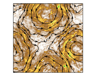
The vertical variation of the r.m.s. velocities can be understood from the Ekman pumping mechanism (Guzmán et al. Reference Guzmán, Madonia, Cheng, Ostilla-Mónico, Clercx and Kunnen2021). The velocity magnitudes around a plume site, as depicted in figure 2, can provide further insight into this phenomenon. Here, the conical plume sites can be recognized from the temperature isosurface  $\theta =0.45$ near the lower boundary in figure 2(a). The horizontal convergence (or divergence) of fluid at the sites of the vortical plumes (figure 2b) enhances the horizontal velocity near the wall with the no-slip boundary condition compared to the free-slip cases in figure 1(a). This fluid then gains vertical acceleration towards the bulk, resulting in higher vertical velocities (figure 2c), as plotted in figure 1(b). Ekman pumping induced by the no-slip boundaries is known to enhance momentum and heat transport (Stellmach et al. Reference Stellmach, Lischper, Julien, Vasil, Cheng, Ribeiro, King and Aurnou2014), and is the reason for the enhanced r.m.s. velocities and temperature fluctuations, especially near the boundaries.

Figure 2. (a) Plume sites visualized by an isosurface of the instantaneous temperature field with  $\theta =0.45$, coloured by the horizontal velocity for the NSC case at
  $\mathcal {R}=3$. A typical plume site in (a), as marked by the dashed rectangle, has been magnified and coloured by horizontal and vertical velocities in (b,c) respectively.
Furthermore, in the inset of figure 1(c), the thermal boundary layer thickness ( $\delta _T$) for the free-slip boundaries (horizontal black dashed line) is about three times higher than the no-slip boundaries (horizontal red dashed line). The thermal fluctuations are enhanced with no-slip boundary conditions, with maximum r.m.s. fluctuation shifting towards the wall. It is noteworthy that changing the boundary conditions can significantly modulate the bulk behaviour apart from the boundary layer dynamics. Also, the effects of changing the kinematic boundary condition on the velocity and thermal fields are more prominent than the magnetic conditions. The mean temperature profile shows a higher temperature gradient near the bottom wall for no-slip conditions (see the inset in figure 1d), with the highest vertical gradient for the NSC case indicating the highest heat transfer from the wall among all the cases at
  $\mathcal {R}=3$ (see § 3.4 for detailed discussion). However, the mean temperature profile and its gradient at the mid-plane remain nearly independent of boundary conditions.
In the present simulations, the magnetic Reynolds number  $Re_m=Re\,Pr_m=u_\tau d/\eta$ (where
  $u_\tau =u_f\langle 2K \rangle ^{1/2}$ is the turbulent velocity scale) has the same value with the Reynolds number
  $Re$, for
  $Pr_m=1$ (see tables 1–4). The Reynolds number increases by an order of magnitude in the range
  $\mathcal {R}=2\unicode{x2013} 20$, indicating increased velocity fluctuations with thermal forcing, irrespective of boundary conditions. The r.m.s. temperature fluctuations also increase monotonically with increased thermal forcing (figure not presented). The decreasing rotational constraint with increasing
  $\mathcal {R}$ leads to decreasing effect of Ekman pumping on the velocity and temperature field. Therefore, the differences between r.m.s. velocity and temperature magnitudes with no-slip and free-slip conditions diminish with increasing
  $\mathcal {R}$. We find LSV in the regime of geostrophic turbulence for FS cases (see tables 2–3 and § 3.4 for details). With this flow structure, the horizontal velocity becomes higher than for all the other cases.
Apart from the velocity and thermal fields, we look into the effect of boundary conditions on the enstrophy, relative helicity and the magnetic field. The vertical variations of horizontally averaged enstrophy, relative helicity, mean and r.m.s. magnetic field strengths are depicted in figures 3(a–d), respectively. In turbulent dynamos, the dynamical alignment of magnetic field lines (Tobias Reference Tobias2021) occurs around the edges of vortices. A measure of the strength of the vortical elements in the flow is given by the enstrophy  $Ek_{\omega }=1/2\,\overline {\omega _i\omega _i}$. The strength of the vortices can decide the extent to which they can deform the magnetic field lines around them, and therefore can be correlated with the local Lorentz force magnitude (Naskar & Pal Reference Naskar and Pal2022). The vorticity fluctuations are enhanced in the bulk, as depicted by the enstrophy, with a more than two orders of magnitude jump near the boundaries (see the inset in figure 3a). The strengths of the vortices are enhanced due to Ekman pumping near the wall. The presence of the energetic vortices near the wall may significantly alter the boundary layer dynamics and the associated heat transfer characteristics of a dynamo compared to the same without the presence of an Ekman layer with free-slip boundaries (Naskar & Pal Reference Naskar and Pal2022).

Figure 3. Vertical variation of the r.m.s. quantities: (a) enstrophy, (b) relative helicity, (c) mean magnetic field, (d) r.m.s. magnetic field at  $\mathcal {R}=3$. All the quantities are averaged in time and in the horizontal directions. The mean and r.m.s. magnetic fields in figures (c) and (d) are plotted using solid lines for x 1-direction and dashed line for x 3-direction.
Another important quantity is the kinetic helicity of the flow, which can induce large-scale mean fields in a dynamo (Tilgner Reference Tilgner2012). The relative kinetic helicity  $\mathcal {H}_r=\overline {u_{i}\omega _{i}}/2(KE_{\omega })^{1/2}$ exhibits the well-known spatial segregation in the vertical direction, as expected in RC, with negative and positive helicity dominating in the bottom and top halves of the domain, respectively (Cattaneo & Hughes Reference Cattaneo and Hughes2006; Schmitz & Tilgner Reference Schmitz and Tilgner2010). Helicity is enhanced by the presence of the wall, where the thermal plumes departing from the boundary layer towards the bulk are spun up by the Coriolis force, due to Ekman pumping (Schmitz & Tilgner Reference Schmitz and Tilgner2010). This phenomenon results in a strong correlation between local velocity and vorticity that leads to a peak of relative kinetic helicity near the wall, as shown in the inset in figure 3(b). However, in the bulk, the relative helicity magnitude remains similar for all the dynamo simulations.
Additionally, we look into the effect of boundary conditions on the strength and structure of the magnetic field produced by the dynamos. The horizontally averaged mean magnetic field is plotted in figure 3(c), which illustrates the dependence on magnetic boundary conditions, even in the bulk. NSC conditions lead to the highest mean field magnitude among all the cases. It should be noted here that for perfectly conducting boundaries, the vertical component of the mean magnetic field,  $\bar {B}_3$, is identically zero by the definition of averages (2.9) and the solenoidal field condition (2.1), so that the mean field remains horizontal. Conversely, the mean field is three-dimensional with a purely vertical field at the boundaries for pseudo-vacuum conditions. However, at
  $\mathcal {R}=3$, the mean vertical field remains small compared to the horizontal field for NSV and FSV conditions in figure 3(c). We find that the vertical averages of
  $\bar {B}_{1}$ and
  $\bar {B}_{2}$ are two orders of magnitude smaller than the maximum mean field strength for NSC and FSC boundary conditions. Jones & Roberts (Reference Jones and Roberts2000) also demonstrate analytically that for perfectly conducting boundaries, the vertical averages of the mean magnetic fields are zero. However, NSV and FSV boundaries do not satisfy this condition.
In contrast to the mean-field, the fluctuating part of the magnetic field is always three-dimensional, with all components non-zero except at the wall. The r.m.s. values of the fluctuating horizontal and vertical magnetic fields are plotted in figure 3(d). For  $\mathcal {R}=3$, the fluctuating magnetic field is approximately one order of magnitude stronger than the mean magnetic field. However, lower thermal forcing can generate strong, large-scale mean magnetic fields, as reported in earlier studies (Stellmach & Hansen Reference Stellmach and Hansen2004; Tilgner Reference Tilgner2012; Naskar & Pal Reference Naskar and Pal2022). Dynamos with no-slip boundary conditions lead to higher r.m.s. field strength than that with free-slip boundaries. For NSC conditions, a large horizontal r.m.s. field magnitude can be observed near the boundaries. The stretching of the magnetic field lines by the strong vortices near the wall results in an increase in the r.m.s. field strength. As the magnetic field has to remain parallel to a perfectly conducting surface, it remains trapped near the walls, leading to a build-up of the magnetic field strength (St Pierre Reference St Pierre1993). Recently, the DNS of Kolhey et al. (Reference Kolhey, Stellmach and Heyner2022) have confirmed this build-up of the field for NSC conditions that creates a stringent resolution requirement near the boundaries. The overall structure and magnitude of the magnetic field, both in the bulk and near the boundaries, are strongly dependent on the combination of kinematic and magnetic boundary conditions for all
  $\mathcal {R}$.
In tables 1–4, the traditional Elsasser number  $\varLambda _{tr}=\sigma B_{\tau }^{2}/2\rho \varOmega =2\,Ra\,EM\,Pr_m/Pr$ provides a non-dimensional measure of the magnetic field strength, where
  $M=1/2\langle B_iB_i\rangle$ is the volume-averaged magnetic energy, and
  $B_{\tau }=\sqrt {\rho \mu }\,u_{f}(2M)^{1/2}$ is a characteristic value of the magnetic field. The magnetic field strength of the dynamos rises monotonically with increasing thermal forcing for all boundary conditions. However, the relative mean field strength
  $\bar {M}/M$, where
  $\bar {M}=1/2\langle B_i\rangle \langle B_i\rangle$, is found to decrease (tables 1–4) with increasing
  $\mathcal {R}$, indicating a shift towards small-scale dynamo action with increasing thermal forcing (Tilgner Reference Tilgner2012, Reference Tilgner2014). We find ‘energetically robust’ dynamos at
  $\mathcal {R}=2$ (corresponding to
  $\widetilde {Re_m}=Re_{m}\,Ek^{1/3}=O(1)$) with significant
  $\bar {M}/M$, confirming the findings of Yan & Calkins (Reference Yan and Calkins2022b). The present study shows that such dynamos are generated for
  $\widetilde {Re_m}\approx O(1)$, irrespective of the boundary conditions.
3.2. Force balance
Now we look into the dynamical balances of the dynamos with different kinematic and magnetic boundary conditions at  $\mathcal {R}=3$. Figure 4 shows the vertical variation of the horizontally averaged forces, evaluated from the r.m.s. values of each term in the momentum equation (2.2) (Guzmán et al. Reference Guzmán, Madonia, Cheng, Ostilla-Mónico, Clercx and Kunnen2021; Yan et al. Reference Yan, Tobias and Calkins2021). The figure presents the forces for no-slip (figures 4a,c,e) and free-slip (figures 4b,d, f) boundary conditions at
  $\mathcal {R}=3$. Here, the RC simulation results (figures 4a,b) are used as a reference to interpret the results for DC simulations with perfectly conducting (figures 4c,d) and pseudo-vacuum (figures 4e, f) boundary conditions. At
  $\mathcal {R}=3$, we get the thermal and Ekman boundary layer thickness as
  $\delta _T=0.011$ and
  $\delta _{Ek}=0.002$ for the no-slip cases, whereas the thermal layer thickness increases to
  $\delta _T=0.034$ for the free-slip cases. The near-wall regions are magnified in the insets, with the velocity and thermal boundary layer edges marked by the black horizontal dashed and dash-dot lines, respectively, in figure 4(a). For all the cases shown in this plot, the leading-order balance between Coriolis and pressure force indicates a geostrophic state in the bulk. For non-magnetic rapid RC, geostrophic balance in the bulk has been confirmed by DNS (Guzmán et al. Reference Guzmán, Madonia, Cheng, Ostilla-Mónico, Clercx and Kunnen2021), apart from reduced-order models in the rapidly rotating limit (Julien et al. Reference Julien, Rubio, Grooms and Knobloch2012b). The DNS study of rapidly rotating DC by Yan & Calkins (Reference Yan and Calkins2022a) has also found leading-order geostrophic balance, for FSV conditions. Departure from the geostrophic state due to the other forces, which constitute a lower-order quasi-geostrophic balance, makes turbulent convection possible. In the non-magnetic simulations (NS and FS) in figures 4(a) and 4(b), the geostrophic and quasi-geostrophic forces behave similarly except near the boundaries (see insets), where the viscous force break the geostrophic balance and dominate the other quasi-geostrophic forces (inertia and buoyancy) in the Ekman layer near the plates with the no-slip boundary condition.

Figure 4. Vertical variation of forces for (a) NS, (b) FS, (c) NSC, (d) FSC, (e) NSV, ( f) FSV cases at  $\mathcal {R}=3$. The horizontally averaged force distribution is shown in the bulk and near the bottom plate (inset).
For the dynamo simulations, the Lorentz force exerted by the magnetic field on the flow also enters the quasi-geostrophic balance. For the NSC case, as shown in figure 4(c), the Lorentz force is minimum at the mid-plane, which increases towards the walls to dominate the quasi-geostrophic balance for  $x_3\leqslant -0.25$. Inside the thermal boundary layer, the Lorentz force increases to the same order of magnitude as the Coriolis force, and eventually becomes the highest force at the wall. This is reflected by the value of the local Elsasser number
  $\varLambda _T$ (the ratio of the r.m.s. magnitudes of the Lorentz and the Coriolis forces at the edge of the thermal boundary layer, calculated from the horizontally averaged variation of the two forces), as presented in tables 1–4. This increase in the Lorentz force at the thermal boundary layer edge leads to a local magnetorelaxation of the thermal boundary layer, which results in increased turbulence and heat transport (Naskar & Pal Reference Naskar and Pal2022). Similar behaviour of the Lorentz force near the boundary was found in the range
  $\mathcal {R}=3\unicode{x2013} 5$ for the NSC cases. However, no such enhancement of Lorentz force is found in the dynamo simulations with any other combinations of the boundary conditions. For the NSV case in figure 4(e), the Lorentz force is higher than the other quasi-geostrophic forces in the bulk, but decreases inside the thermal layer. Unlike the NSC case, the Lorentz force in the NSV case keeps decreasing towards the Ekman layer, where the viscous force dominates. The volume-averaged ratio of the Lorentz and Coriolis forces,
  $\varLambda _V$, is also presented in tables 1–4. This volume-averaged Elsasser number reaches a maximum near
  $\mathcal {R}=4$ for the NSV case in table 2. The Lorentz force inside the thermal layer is one order of magnitude smaller than the other quasi-geostrophic forces for the FSC case in figure 4(d), making the near-wall balance similar to the non-magnetic RC (FS). Though the Lorentz force has magnitude similar to that of the viscous force in the bulk for the FSV cases in figure 4( f), it becomes the smallest force inside the thermal boundary layer, again making the balance similar to the FS case near the walls. Therefore, our results corroborate the finding of Yan & Calkins (Reference Yan and Calkins2022a), that the Lorentz force acts as a small perturbation in the force balance, with magnitude similar to that of the viscous force, for the FSV boundaries. These results illustrate the dependence of the dynamical balance of the dynamo on the imposed boundary conditions, especially near the boundary. Also, the dynamo simulations with no-slip conditions exhibit distinctive balance compared to the non-magnetic convection inside the thermal boundary layer. In contrast, the dynamical balance in the thermal layer is similar to RC for free-slip boundary conditions with negligible contribution from the Lorentz force. The magnetic boundary condition decide the magnitude and vertical distribution of the Lorentz force in the dynamos.
The force balance in the NSC case at  $\mathcal {R}=3$ exhibits some interesting features near the boundary layer, as shown in figure 4. This case can be analysed in more detail from figure 5, where the horizontal and vertical balances are illustrated separately and compared with the NS case. As the rotation axis is aligned with the vertical, the Coriolis force acts only in the horizontal planes, whereas the buoyancy force is purely vertical. In the non-magnetic NS case, the leading-order horizontal balance is geostrophic between the Coriolis and pressure forces, as depicted in figure 5(a). The ageostrophy, as defined by the difference between the two forces, is balanced by the inertia and viscous forces. Near the walls, there is a sharp increase in the ageostrophy, balanced by the viscous force, indicating a loss of geostrophic balance inside the viscous boundary layers, as seen in the inset of figure 5(a) (see also Guzmán et al. Reference Guzmán, Madonia, Cheng, Ostilla-Mónico, Clercx and Kunnen2021). Among the vertical forces in figure 5(b), the vertical pressure gradient is balanced by the inertia and buoyancy forces in the bulk where the viscous forces remain small.

Figure 5. Vertical variation of the force components for (a,b) NS and (c,d) NSC cases. (a,c) Horizontal components of the forces  $F_h=\sqrt {F^2_{x_1}+F^2_{x_2}}$; (b,d) vertical components (
 $F_{x_3}$). The horizontally averaged force distribution is shown here at
  $\mathcal {R}=3$ both in the bulk, and near the bottom plate (inset).
In the NSC case, the leading-order balance remains geostrophic in the horizontal direction, as presented in figure 5(c). However, the ageostrophy is much higher than the NS case due to magnetorelaxation of the Taylor–Proudman theorem in the presence of the Lorentz force. The ageostrophic component is balanced by the Lorentz and inertial forces in the bulk. In the vertical direction, the pressure force is balanced by the Lorentz, buoyancy and inertial forces, as shown in figure 5(d). We note here that the horizontal components of the forces are always higher than the vertical forces, with the force magnitudes enhanced near the boundaries for all the cases. The flow velocities gradually come to zero inside the Ekman layer, resulting in an increase in the pressure at the boundary. Furthermore, the details of the force balance, especially the role of inertia, depend on  $\mathcal {R}$. With increase in
  $\mathcal {R}$, the inertial force eventually dominates the quasi-geostrophic balance, as observed for
  $\mathcal {R}=20$ in figures 6(a) and 6(b) for the NS and NSC cases, respectively. This increase in inertia with thermal forcing corroborates the findings of Guzmán et al. (Reference Guzmán, Madonia, Cheng, Ostilla-Mónico, Clercx and Kunnen2021), and is a common feature among all boundary conditions. The local magnetorelaxation of the rotational constraint in the thermal boundary layer, as a mechanism for increase in heat transfer in the NSC case compared to the NS case, becomes gradually ineffective with increasing
  $\mathcal {R}$. This is because the increased inertia, rather than the Lorentz force, breaks the Taylor–Proudman constraint for both RC and DC simulations, irrespective of boundary conditions.

Figure 6. Vertical profiles of the forces for (a) NS, (b) NSC cases at  $\mathcal {R}=20$. The horizontally averaged force distribution is shown in the bulk and near the bottom plate (inset).
3.3. Energy budget
We further analyse the various energetic terms in the TKE budget equation (A1) to illustrate the generation of TKE from thermal forcing, and its dissipation and conversion to magnetic energy for elucidating the turbulent dynamo mechanism. The significance of the TKE budget terms and their dependence on the boundary conditions have been explored, with particular attention paid to the near-wall features. In figure 7, the various terms in the TKE budget equation (see Appendix A) are plotted with the near-wall variation shown in the inset. All the terms are averaged in the horizontal planes, and their variation in the vertical direction is shown at  $\mathcal {R}=3$ with varying boundary conditions. For the NS and FS cases, in figures 7(a) and 7(b), the primary energy balance is between the buoyant production (
 $\mathcal {B}$) and viscous dissipation (
 $\epsilon _v$). The transport term
  $\partial \mathcal {T}_j/\partial x_j$ acts to redistribute the energy and becomes zero when averaged over the volume. This term includes the combined effect of diffusive transport, pressure transport and third-order correlation terms (see (A3)). A detailed discussion of a typical energy budget in RC with the individual treatment of these terms can be found in Kunnen, Geurts & Clercx (Reference Kunnen, Geurts and Clercx2009). In the absence of a mean flow, the shear production term
  $P$ is zero, whereas the unsteady term
  $\partial K/\partial t$ also becomes zero in the statistically stationary state. In the bulk, for the non-magnetic RC cases (as shown in figures 7a,b), some part of the TKE generated from the buoyant production is converted to thermal energy by viscous dissipation, and the rest is redistributed by the transport term. Near the boundaries, this transport of kinetic energy term transfers energy from the bulk towards the boundary layers, which undergoes viscous dissipation. Hence the primary balance is between the dissipation and transport terms near the plates. Due to the presence of viscous Ekman layers in the NS case, the viscous dissipation (and therefore the kinetic energy transport) increases by two orders of magnitude near the plates compared to their bulk values, as shown in the inset of figure 7(a). Such an order of magnitude jump is not present for the FS case in figure 7(b) owing to the absence of the Ekman boundary layer.

Figure 7. Vertical variation of TKE budget terms at  $\mathcal {R}=3$ for both no-slip (a,c,e) and free-slip (b,d, f) boundaries. Energy budget terms are presented for non-magnetic simulations (a,b) as well as dynamo simulations with both perfectly conducting (c,d) and pseudo-vacuum (e, f) conditions. The horizontally averaged budget terms in (A1) are averaged in time. The profiles near the bottom wall are magnified in the insets. The balance terms signify the difference between the left- and right-hand sides of (A1), and indicate sufficient accuracy of the present calculations.
For the dynamos, the magnetic production of TKE ( $\mathcal {P}$) appears in (A1) to represent the work done by the Lorentz force on the velocity field to produce TKE. A negative value of this term indicates transfer of energy from the velocity field to the magnetic field, and vice versa. This term is responsible for converting some part of the kinetic energy to magnetic energy to sustain dynamo action. For all the dynamo cases (NSC, NSV, FSC and FSV),
  $\mathcal {P}$ appears as an additional sink of TKE that balances the buoyant production of kinetic energy together with viscous dissipation. The behaviour of magnetic production is similar to viscous dissipation for the NSC case. Here, the budget terms show a peak near the edge of the Ekman layer, as shown in the inset of figure 7(c). For the NSV boundary condition in figure 7(e), the magnetic production term is not significant near the mid-plane but increases towards the boundary to reach a peak near
  $x=\pm 0.4$ before it decreases to zero at the wall. For FSC and FSV conditions, the contribution from this term is not significant to the overall budget, as plotted in figures 7(d) and 7( f). This magnetic production term in the TKE budget comprises of three components,
  $\mathcal {P}_1$,
  $\mathcal {P}_2$ and
  $\mathcal {P}_3$, as expressed in (A4a–c). Out of these, the first two magnetic production terms involving the mean magnetic field and its gradients (
 $\mathcal {P}_1$ and
  $\mathcal {P}_2$) are found to be small compared to
  $\mathcal {P}_3$ at
  $\mathcal {R}=3$. It should be noted here that for lower convective supercriticality, the mean magnetic field may become strong compared to the turbulent magnetic field, and therefore the terms
  $\mathcal {P}_1$ and
  $\mathcal {P}_2$ may contribute significantly to magnetic production. The transport of kinetic energy by the mean and fluctuating magnetic fields, as represented by the last two terms in the right-hand side of (A3), are also found to be small compared to the pressure transport and turbulent transport terms (figure not presented).
The dominant term among the magnetic production terms,  $\mathcal {P}_3$, represents the work done by the fluctuating magnetic field on the fluctuating velocity field to produce TKE. It is interesting to study this term for elucidating the mechanism of energy exchange between these two vector fields. The nine components of this term are represented by
  $\mathcal {P}^{ij}_3=\overline {B^{\prime }_{i}B^{\prime }_{j}\,\partial u^{\prime }_{i}/\partial x_{j}}$ in figure 8 for the NSC and NSV cases where magnetic production makes a significant contribution to the TKE budget. Among these nine components, the three terms involving the vertical gradient of the fluctuating velocity field,
  $\mathcal {P}^{i3}_3=\overline {B^{\prime }_{i}B^{\prime }_{3}\,\partial u^{\prime }_{i}/\partial x_{3}}$ (where
  $i=1,2,3$) are small due to the Taylor–Proudman constraint on the velocity field imposed by rotation that suppresses changes in the vertical direction. Interestingly, for the NSC case, there are components with both positive and negative values in figure 8(a). Here, the components
  $\mathcal {P}^{11}_3$ and
  $\mathcal {P}^{21}_3$ become positive away from the mid-plane, indicating a transfer of energy from the magnetic field to the velocity field. Vertical variations of the terms
  $\mathcal {P}^{12}_3$ and
  $\mathcal {P}^{22}_3$ are similar but opposite, with negative values away from the mid-plane indicating transfer of energy from the velocity to the magnetic field. The last two negative terms, being larger than the positive terms, provide a bias in the direction of energy transfer so that the system can extract kinetic energy of the fluid and convert it to magnetic energy to sustain dynamo action. However, at the mid-plane, all the terms are negative. Near the wall, these four terms exhibit peaks near the edge of the Ekman boundary layer where the values are two orders of magnitude higher than at the mid-plane. The two remaining terms,
  $\mathcal {P}^{31}_3$ and
  $\mathcal {P}^{32}_3$, are small compared to the dominant terms near the wall, but contribute most to the energy transfer at the mid-plane. In the NSV case, all the components of work done by the Lorentz force
  $\mathcal {P}^{ij}_3$ are negative, indicating unidirectional energy transfer from the velocity field to the magnetic field. This demonstrates that the imposed boundary conditions dictate the energy exchange mechanism between the velocity and magnetic fields, both in the bulk and near the boundaries.

Figure 8. Variation of the magnetic production terms for (a) NSC and (b) NSV cases at  $\mathcal {R}=3$. The components of the work done by the Lorentz force
  $\mathcal {P}_3$ are represented by the colours: black for
  $i=1$, red for
  $i=2$, and blue for
  $i=3$. Here, the lines with
  $+$ symbols and filled and open circles represent
  $j=1$,
  $j=2$ and
  $j=3$, respectively.
The volume-averaged budget of turbulent magnetic energy, reduces to a balance between the magnetic energy production and the Joule dissipation,  $\langle \mathcal {P}\rangle =\langle \epsilon _j\rangle$, for statistically stationary turbulence. This signifies that the part of TKE converted to magnetic energy ultimately converts to thermal energy via Joule dissipation. The Ohmic fraction, defined by the ratio of Joule dissipation to total dissipation
  $\langle \epsilon _j\rangle /\langle \epsilon \rangle$, is presented in tables 1–4. The Ohmic fraction does not show any particular trend in the range
  $\mathcal {R}=2\unicode{x2013} 20$. The global energy balance between buoyant production
  $\langle \mathcal {B}\rangle$ and total dissipation
  $\langle \epsilon \rangle$ is also presented in these tables, where the values have been scaled by a factor
  $10^4$. The difference between the two terms never exceeds
  $5\,\%$ of
  $\langle \mathcal {B}\rangle$, indicating the accuracy of the present DNS in capturing all the energy-containing scales. The vertical trends of the terms in the TKE equation remain similar to those presented in figure 7 over the range of thermal forcing studied here. The volume-averaged buoyancy flux and dissipation increase by an order of magnitude in the range
  $\mathcal {R}=2\unicode{x2013} 20$.
3.4. Heat transfer behaviour
Finally, we study the heat transfer behaviour of the dynamo simulations with increasing thermal forcing under the influence of different boundary conditions. In figure 9, the Nusselt number ratio  $Nu/Nu_0$ signifies the change in heat transport in DC simulations due to dynamo action compared to the non-magnetic RC simulations. For NSC, a peak is found near
  $\mathcal {R}=3$, with more than
  $72\,\%$ enhancement in heat transfer. A peak in Nusselt number ratio is also found for the NSV case at
  $\mathcal {R}=3$, with a
  $41\,\%$ increase in heat transport compared to non-magnetic RC. For FSC and FSV cases, the heat transfer ratio also peaks at
  $\mathcal {R}=4$ and
  $\mathcal {R}=3$, with enhancement up to
  $56\,\%$ and
  $34\,\%$, respectively. The ratio of viscous dissipation in the DC and RC simulations
  $\langle \epsilon _v\rangle /\langle \epsilon _0\rangle$ is also presented in tables 1–4, which shows a similar trend with the Nusselt number ratio. The peaks in heat transfer ratio and the viscous dissipation ratio occur at the same value of
  $\mathcal {R}$. We note here that the overall energy balance of the system leads to an exact relation between the Nusselt number and the total dissipation,
  $Nu=1+\sqrt {Ra\,Pr}\,\langle \epsilon \rangle$. Hence the dissipation ratio should behave similarly to the Nusselt number ratio with varying
  $\mathcal {R}$, as seen in tables 1–4. A local magnetorelaxation of the rotational constraint, due to enhanced Lorentz force in the thermal boundary layer (see figure 4c), has been proposed to be the reason for the rise in heat transfer in the NSC case (Naskar & Pal Reference Naskar and Pal2022). However, the build-up of the Lorentz force required for this magnetorelaxation process is not present for any other combinations of the boundary conditions (see figure 4). Notably, in the NSV case, the Lorentz force in the bulk is higher compared to the other cases in figure 4(e). Indeed, the volume-averaged Elsasser number
  $\varLambda _V$ in table 2 shows a peak at
  $\mathcal {R}=3$ that correlates well with the heat transfer behaviour. Therefore, the global relaxation of the Taylor–Proudman constraint is a possible mechanism for the heat transfer enhancement. For the free-slip cases, the heat transfer enhancement in dynamos is achieved by suppression of LSV by the small-scale magnetic field, as discussed in the next paragraph. It is interesting to note that the peak in heat transfer ratio appears within a narrow range of thermal forcing
  $\mathcal {R}=3\unicode{x2013} 4$, depending on the conditions at the boundary. Further investigations will be necessary to elucidate the appearance of the peak in heat transfer ratio for different boundary conditions. However, the heat transport properties of the dynamo depend on the boundary conditions and the associated dynamical balances both in the bulk and in the boundary layer.

Figure 9. Variation of the Nusselt number ratio  $Nu/Nu_0$ as a function of the thermal forcing for different boundary conditions. Here,
  $Nu_0$ represents the Nusselt number for the non-magnetic RC simulations.
The heat transfer enhancement in the dynamos with free-slip boundary conditions with respect to non-magnetic RC can be attributed to the absence of LSV in the former. In the FS cases, we find the presence of depth-independent, long-lived (compared to the free-fall time scale) LSV for  $\mathcal {R}\geqslant 4$, corroborating the findings of Guervilly et al. (Reference Guervilly, Hughes and Jones2014). Similar to freely decaying two-dimensional turbulence, the formation of LSV in RC involves an upscale energy transfer from the convective eddies to large-scale barotropic modes (Favier, Silvers & Proctor Reference Favier, Silvers and Proctor2014; Rubio et al. Reference Rubio, Julien, Knobloch and Weiss2014). The flow associated with these structures is nearly two-dimensional, which can be visualized from the contours of horizontal TKE,
  $K_h=1/2(u_{1}^2+u_{2}^2)$, which tends to be high in the shear layer around the core of these vortices, as shown in figure 10(a) for
  $\mathcal {R}=4$. An animation of the LSV, as visualized by the time evolution of the
  $K_h$ contours, can be found in the supplementary movie available at https://doi.org/10.1017/jfm.2022.841. Here, we find a pair of cyclonic and anti-cyclonic vortices centred around
  $(0.48,0.87)$ and
  $(0.93,0.34)$, respectively, as depicted in the horizontal mid-plane at
  $x_3=0.5$. The degree to which the two-dimensionality of the flow has been induced by the presence of an LSV can be measured by the ratio
  $\tau =\langle u_{1}^2+u_{2}^2+u_{3}^2\rangle /3\langle u_{3}^2\rangle$, as reported in tables 1–4. The kinetic energy ratio for the RC simulations
  $\tau _{0}$ is also reported in tables 2 and 3 for the NS and FS cases, respectively. As the kinetic energy associated with the horizontal flow in the LSV is higher than the kinetic energy in the vertical flow, the value of
  $\tau$ increases to values much higher than unity in the FS cases for
  $\mathcal {R}\geqslant 4$. We have also found LSV with no-slip boundary conditions without magnetic field (NS case) for
  $\mathcal {R}=10$ and
  $20$, which supports the findings of Guzmán et al. (Reference Guzmán, Madonia, Cheng, Ostilla-Mónico, Clercx and Kunnen2020) that LSV appear in RC irrespective of the kinematic boundary condition. However, the presence of no-slip boundaries suppresses the formation of LSV until higher convective supercriticality (
 $\mathcal {R}\geqslant 10$) compared to the free-slip cases (
 $\mathcal {R}\geqslant 4$).

Figure 10. Contours of horizontal TKE,  $K_h=1/2(u_{1}^2+u_{2}^2)$ for (a) FS and (b) FSC cases at
  $\mathcal {R}=4$. The instantaneous plots are shown in the horizontal mid-plane at
  $x_3=0.5$ to illustrate the presence of LSV in (a), which is superimposed with streamlines. The dynamo simulation with FSC conditions generates small-scale velocity and magnetic fields as illustrated by contours of TKE and magnetic field
  $B_1$ in (b,c), respectively. The vertical temperature gradients at
  $\mathcal {R}=4$ are shown in (d) for the free-slip cases. The mean temperature profile near the lower wall is also shown in the inset.
Guervilly et al. (Reference Guervilly, Hughes and Jones2017) reported that for  $Re_m\geqslant 550$, the formation of LSV can be suppressed by the presence of a small-scale magnetic field. Such a field acts to disrupt the correlations between the convective vortices that in turn hinder the upscale transfer of energy. This should be the reason why we do not find any LSV in our dynamo simulations with free-slip conditions that operate for
  $Re_m\geqslant 641$. The combined effect of the no-slip boundary condition and the presence of a magnetic field has suppressed the LSV in the NSC and NSV cases as well, as reflected by the value of
  $\tau$ in tables 1 and 2. Maffei et al. (Reference Maffei, Calkins, Julien and Marti2019) used an asymptotic magnetohydrodynamic model to study the effect of an imposed magnetic field on the inverse cascade of energy in the turbulent geostrophic regime of RC. The possibility of occurrence of LSV in the presence of the magnetic field was quantified by an interaction parameter
  $N$, which signifies the relative strengths of the Lorentz force and the non-linear advection. For
  $N\geqslant 0.013$, the magnetic field disrupts the upscale energy transfer, hence LSV can be present only below this limit. We have calculated the interaction parameter as a ratio of the volume-averaged r.m.s. magnitudes of the Lorentz force and the nonlinear advection terms, and found the ratio to be of
  $O(10^{-1})$ for all our dynamo simulations. Though the self-excited magnetic fields in our dynamo simulations are not directly comparable to the externally imposed field used by Maffei et al. (Reference Maffei, Calkins, Julien and Marti2019), the magnetic quenching of the inverse cascade is a plausible mechanism for the disappearance of LSV in our dynamo simulations. The horizontal TKE and the
  $x_1$ component of the magnetic field for FSC cases, as depicted in figures 10(b) and 10(c), show small-scale fields without any trace of LSV. The presence of LSV can disrupt the vertical mixing by transferring energy to horizontal barotropic modes (Guervilly et al. Reference Guervilly, Hughes and Jones2014). In figure 10(d), this phenomenon results in an increased gradient of temperature in the bulk for the FS case with LSV, compared to the FSC and FSV cases without LSV. The temperature profiles near the wall (see inset) show higher thermal boundary layer thickness in the FS case compared to the dynamo cases, indicating a decrease in heat transfer efficiency near the wall in the FS case. The thermal plumes near the wall get swept away by the horizontal flow associated with LSV, which can interrupt the vertical transport of heat by the plumes, leading to a decrease in the heat transfer efficiency.
4. Conclusions
We have performed high-fidelity DNS of dynamos driven by rapidly rotating RBC under four combinations of kinematic and magnetic boundary conditions. The simulations are performed in the rotation-dominated regime  $\mathcal {R}=2\unicode{x2013} 20$ at a fixed rotation rate
  $Ek=5\times 10^{-7}$ and fluid properties
  $Pr=Pr_{m}=1$. The dynamo simulations with the no-slip and free-slip kinematic boundary conditions combined with the perfectly conducting and pseudo-vacuum magnetic boundary conditions (NSC, NSV, FSC and FSV) are compared against non-magnetic simulations (NS and FS) to study the impact of the dynamo action on the convective flow properties. Our previous study (Naskar & Pal Reference Naskar and Pal2022) reported the existence of optimal heat transfer enhancement with respect to non-magnetic convection due to dynamo action for NSC boundary conditions at
  $\mathcal {R}=3$. Therefore, we have chosen this case to compare the statistics of the velocity, thermal and magnetic fields in addition to the dynamical balance, energy budget and heat transfer behaviour of the dynamos.
The flow and thermal field of the dynamos, apart from the structure of the magnetic field, are found to depend on the boundary conditions. Ekman pumping significantly enhances the velocity and thermal fluctuations in the dynamos, increasing the r.m.s. velocities and temperatures both in the bulk and near the boundaries. It also leads to a three orders of magnitude increase in enstrophy, signifying increased strength of the vortical plumes inside the Ekman layer with the no-slip boundary condition. The relative helicity also exhibits a peak near the Ekman layer, illustrating strong correlations between the velocity and vorticity fields. The perfectly conducting boundary conditions can trap the magnetic field near the boundaries to prevent its escape and make it purely horizontal. This leads to a jump of r.m.s. horizontal field strength near the boundaries for the NSC case. The r.m.s. field strength remains higher than the mean field for all combinations of the boundary conditions in the investigated range of thermal forcing.
The leading-order force balance in the dynamos remains geostrophic, similar to our non-magnetic RC simulations, irrespective of the boundary conditions. At  $\mathcal {R}=3$, the quasi-geostrophic balance corresponds to a Coriolis-inertial-Archimedean force balance between the ageostrophic part of Coriolis, inertia and buoyancy forces in the non-magnetic simulations. The extent to which the Lorentz force modulates the quasi-geostrophic balance is decided by the boundary conditions in the dynamo simulations. For NSC conditions, a build-up of the Lorentz force is seen near the walls, whereas this force dominates the quasi-geostrophic balance in the bulk for NSV conditions. For free-slip conditions, the Lorentz force is much weaker compared to the no-slip dynamos.
The budget of TKE for the non-magnetic cases exhibits an overall balance between the buoyant production and viscous dissipation. For the NS case, the viscous dissipation increases by two orders of magnitude from its bulk value due to viscous action inside the Ekman layer. For the dynamo simulations, some part of the TKE is converted to magnetic energy via work done by the Lorentz force, which is ultimately converted to thermal energy by the Joule dissipation. This additional term, signifying the production of magnetic energy in the dynamo simulations, is considerably weaker with free-slip boundaries than no-slip boundaries. A break up of the components that constitute this production of magnetic energy term (which can also be interpreted as the work done by the Lorentz force on the flow) reveals that the energy flows both ways, from the velocity field to the magnetic field and vice versa, when NSC conditions are imposed at the boundary. Conversely, the flow of energy is unidirectional, from kinetic energy to magnetic energy, when the NSV boundary condition is used, indicating the decisive role of the boundary conditions on the mechanism of energy transfer.
Another interesting finding of our study is the enhancement of heat transfer in the DC simulations with respect to the non-magnetic RC simulations. The heat transfer enhancement reaches a peak in the range  $\mathcal {R}=3\unicode{x2013} 4$ for all the combinations of boundary conditions. The magnetorelaxation of the rotational constraint by the Lorentz force is the mechanism for heat transfer enhancement for the no-slip cases, whereas for the free-slip dynamos, the suppression of LSV by magnetic field is found to be the reason behind the increased efficiency of heat transport. We have found the LSV in our non-magnetic simulations that are known to deteriorate the heat transfer, as reported in the literature (Guervilly et al. Reference Guervilly, Hughes and Jones2014). By comparing our results with the existing literature, we conclude that the magnetic quenching of LSV by the magnetic field is a possible reason for the heat transfer enhancement in our free-slip dynamo simulations. An interesting extension of the present study will be the search for power-law scaling of the heat transfer and flow speed with the thermal forcing in such convection-driven dynamos, and the effect of boundary conditions on the power-law exponent and the prefactor.
Finally, we would like to point out that the near-wall force balance and the heat transfer behaviour of rotating DC should also depend on  $Pr$, along with the boundary conditions. The length scale at which the Lorentz force enters the force balance (Aurnou & King Reference Aurnou and King2017; Schwaiger, Gastine & Aubert Reference Schwaiger, Gastine and Aubert2019), apart from its dependence on
  $Pr_m$ (if any), also warrants future investigations.
Supplementary movie
A supplementary movie depicting large-scale vortices is available at https://doi.org/10.1017/jfm.2022.841.
Funding
We gratefully acknowledge the support of the Science and Engineering Research Board, Government of India grant no. SERB/ME/2020318. We also want to thank the Office of Research and Development, Indian Institute of Technology, Kanpur for financial support through grant no. IITK/ME/2019194. The support and the resources provided by PARAM Sanganak under the National Supercomputing Mission, Government of India at the Indian Institute of Technology, Kanpur are gratefully acknowledged.
Declaration of interests
The authors report no conflict of interest.
Author contributions
The authors contributed equally to analysing data and reaching conclusions, and in writing the paper.
Appendix A
The TKE equation for a rapidly rotating dynamo can be derived by including the terms involving work done by the Lorentz force. We note here that the Coriolis force is a pseudo-force and does not enter the balance directly. The evolution of the horizontally averaged TKE (see § 3.1 for the definition of the averages) can be written as
 \begin{equation} \frac{{\rm d}K}{{\rm d}t}={-}P+\mathcal{B}-\epsilon_v-\frac{\partial\mathcal{T}_{j}}{\partial x_j}+\mathcal{P}, \end{equation}
where
 \begin{equation} K=\frac{1}{2}\,\overline{u^{\prime}_i{}u^{\prime}_i{}},\quad P={-}\overline{u^{\prime}_iu^{\prime}_j}\,\frac{\partial\overline{u_i}}{\partial x_j},\quad \mathcal{B}=\overline{u^{\prime}_3\theta^{\prime}},\quad \epsilon_v=\sqrt{\frac{Pr}{Ra}}\,\overline{\frac{\partial u^{\prime}_i}{\partial x_j}\,\frac{\partial u^{\prime}_i}{\partial x_j}} \end{equation}
are the TKE, shear production, buoyancy flux and viscous dissipation. The transport of  $K$ is
 \begin{equation} \mathcal{T}_j=\overline{u^{\prime}_jp^{\prime}}+\frac{1}{2}\, \overline{u^{\prime}_iu^{\prime}_iu^{\prime}_j}-\sqrt{\frac{Pr}{Ra}}\,\frac{\partial ^2K}{\partial x_j\,\partial x_j}-\overline{B_j}\,\overline{u^{\prime}_i{}B^{\prime}_i}-\overline{u^{\prime}_iB^{\prime}_iB^{\prime}_j}. \end{equation}
 The shear production term  $P$ in (A2b) is negligible in the absence of a mean flow in the present simulations. However, shear production may still arise in the presence of a mean vertical motion through the turbulent transport term in (A3) (Kerr Reference Kerr2001). The last term on the right-hand side of (A1) is the production of
  $K$ due to the work done by the Lorentz force on the flow field:
 \begin{align} \mathcal{P}_{1}={-}\overline{B_j}\,\overline{B^{\prime}_i\,\frac{\partial u^{\prime}_i}{\partial x_j}},\quad \mathcal{P}_{2}=\overline{u^{\prime}_iB^{\prime}_j}\,\frac{\partial \overline{B_i}}{\partial x_j},\quad \mathcal{P}_{3}={-}\overline{B^{\prime}_iB^{\prime}_j\,\frac{\partial u^{\prime}_i}{\partial x_j}},\quad \mathcal{P}=\mathcal{P}_{1}+\mathcal{P}_{2}+\mathcal{P}_{3}. \end{align}
These magnetic production terms  $\mathcal {P}_{1}$ to
  $\mathcal {P}_{3}$ in (A4a–c) represent the exchange of energy between the velocity and the magnetic fields. For example,
  $\mathcal {P}_1$ signifies the production of TKE due to work done by the mean magnetic field on the fluctuating strain rate of the velocity field. Furthermore,
  $\mathcal {P}_2$ represents the production of TKE due to the mean magnetic field gradient, analogous to the shear production term
  $P$ in (A2b). The amplification (or attenuation) of the magnetic energy, due to the work done by stretching (or squeezing) of magnetic field lines by the fluctuating velocity gradients, is represented by the term
  $\mathcal {P}_3$. The terms
  $\mathcal {P}_{1}$ and
  $\mathcal {P}_{2}$, apart from the last two terms in (A3), representing the transport of kinetic energy by the magnetic field, remain small except at
  $\mathcal {R}=2$.


