1. INTRODUCTION
Integration between the Global Positioning System (GPS) and Inertial Navigation Systems (INS) can be used to provide navigation information such as position, velocity and attitude (Chu et al., Reference Chu, Tsai, Chiang and Duong2013). This has been investigated for several years in different applications, such as military, agriculture and so on. In the integrated navigation system, GPS provides highly accurate position and velocity information over long periods, while the INS provides accurate attitude information in the short term. When a GPS receiver is used to obtain position, it needs to receive the satellite signal. In contrast, an INS is a self-contained device for velocity and attitude data. It is clear that integrating GPS and INS can deliver an enhanced performance over the individual systems (Nassar, Reference Nassar2003).
Recently, Precise Point Positioning (PPP) using un-differenced carrier phase and pseudorange observations has been developed to obtain position information at centimetre level accuracy with the advent of precise orbit and clock products (Kouba and Héroux, Reference Kouba and Héroux2001). In PPP applications, an important constraint is the long ambiguity convergence time, usually about 30 minutes under normal Global Navigation Satellite System (GNSS) observation conditions (Bisnath and Gao, Reference Bisnath and Gao2009). If there is cycle slip, the ambiguity parameter needs to be re-initialised. Cycle slip detection and repair is a key step for PPP data processing. Some methods of cycle slip detection and repair for PPP have been proposed. The problem of detection and identification of cycle slip in carrier phase observation was dealt with by applying the Bayesian theory (de Lacy et al., Reference de Lacy, Reguzzoni, Sansò and Venuti2008). In integration of the ionospheric total electron contents rate and Melbourne-Wübbena (MW) linear combination, one algorithm was proposed to uniquely identify the cycle slip on both L1 and L2 frequencies (Liu, Reference Liu2011). A weighted factor which is tightly related to the GPS satellite elevation angle was introduced in the cycle slip identification process and a modified TurboEdit algorithm (Blewitt, Reference Blewitt1990) was proposed (Miao et al., Reference Miao, Sun and Wu2010). A Forward and Backward Moving Window Averaging (FBMWA) scheme and a Second-order, Time-difference Phase Ionospheric Residual (STPIR) scheme were integrated to jointly detect and identify cycle slip (Cai et al., Reference Cai, Liu, Xia and Dai2013). To avoid a loss of lock on GPS signals, a scheme to instantaneously decrease the impacts of signal interruptions (cycle slip) was presented according to a time-differenced method in a least-squares adjustment (Banville and Langley, Reference Banville and Langley2009). The values of cycle slip could be estimated and fixed with the LAMBDA technique by exploiting a cascade cycle slip resolution algorithm (Zhang and Li, Reference Zhang and Li2012). A geometry-based approach with rigorous handling of the ionosphere is used to detect cycle slip (Banville and Langley, Reference Banville and Langley2013). A new scheme using a new single-frequency instantaneous cycle slip detection and correction algorithm based on optimum time differencing of a single-satellite phase-only observation was presented to handle single-frequency positioning challenges (Momoh and Ziebart, Reference Momoh and Ziebart2012). The presence of a new frequency signal introduced more degrees of freedom in the GNSS data combination. More linear combinations of GNSS observations aiming to detect and repair cycle slips in real time were constructed. Results show that these combinations were able to detect and identify all combinations of cycle slip in the three carriers (de Lacy et al., Reference de Lacy, Reguzzoni and Sansò2012). Though more combination observations can be obtained, GNSS receivers with three-frequency signals are still uncommon. Except for the method with three-frequency signals, the algorithm for cycle slip detection and repair used the pseudorange observation that will introduce high noise and multipath.
Some research has been conducted to integrate the precise point position and inertial navigation system, which will obtain more accurate position and attitude information. For the integrated PPP and INS navigation system, the cycle slip could be detected and repaired with inertial information. The residuals between the Doppler measurement and a calculated Doppler-based INS solution have shown significant changes whenever cycle slip occurs. The short-term stability of the INS is utilised to generate the calculated Doppler, which could reach higher accuracy (Lipp and Gu, Reference Lipp and Gu1994). Combined with GPS, the INS extended the usefulness of the long-range technique filling in gaps in the GPS solution. Further, it was able to improve the reliability of long-range solutions by helping detect and correct cycle slip (Colombo et al., Reference Colombo, Bhapkar and Evans1999). A cycle slip repair algorithm was developed using an available INS to estimate the standard deviation of the decision variables with high accuracy. The integrity of integrated navigation systems was greatly enhanced even under inconvenient conditions with this scheme (Altmayer, Reference Altmayer2000). An algorithm that could effectively detect and identify any type of cycle slip was presented. The algorithm used additional information provided by the INS, and applied a statistical technique known as the Cumulative-Sum (CUSUM) test. In this approach, the cycle slip decision variable was calculated by the INS-predicted position and the CUSUM test was used to identify cycle slip (Lee et al., Reference Lee, Wang and Rizos2003). With the aiding from INS, the proposed method jointly uses Wide-Lane (WL) and Extra Wide-Lane (EWL) phase combinations to uniquely identify cycle slip in the L1 and L2 frequencies, which was able to avoid the relatively high noise and multipath resulting from code measurements. Both high-grade Inertial Measurement Units (IMU) and low-cost Micro-Electromechanical System (MEMS) IMU systems were tested in different field tests and the results indicated that the cycle slip could be detected and repaired with a very high confidence level (Du and Gao, Reference Du and Gao2012). A cycle slip detection algorithm using a low cost inertial navigation sensor and single frequency GPS receiver was proposed with only the precise relative position between GPS epochs. An inertial navigation sensor was used because it had a good performance over a short period (Younsil et al., Reference Younsil, Junesol, Ho, Byungwoon and Changdon2013).
In the present study, an inertial-aided cycle slip detection and repair method presented by Colombo et al. (Reference Colombo, Bhapkar and Evans1999) for long-baseline kinematic GPS is applied in PPP/INS tightly coupled navigation and the detailed calculation process is shown to obtain higher accuracy navigation information. The INS-derived geometric range is calculated and introduced the wide-lane combination observation without pseudorange information. Thus the high noise and multipath of pseudorange is avoided. Combining the geometry free combination, a strategy for cycle slip detection and repair is presented. Differing from the method proposed by Du (Reference Du2010), this paper focuses on the error of inertial-aided combination observation. The errors of the traditional MW combination and inertial aided wide-lane combination are analysed and compared. When the INS position is in high accuracy, the inertial aided combination has less error than the MW combination. Therefore, the inertial aided wide-lane combination has advantages over the traditional MW combination for GPS observation with high sample interval. The paper is divided into seven sections. Following this introduction, the PPP tightly coupled navigation model is overviewed in Section 2. Section 3 describes GPS combination observation for cycle slip detection, including geometry free combination, Melbourne-Wübbena combination and inertial aided wide-lane combination. Section 4 reveals the inertial aided decision variable and its error analysis. The scheme of inertial-aided cycle slip detection and repair is overviewed in Section 5. Test results are then presented and analysed in Section 6, followed by a summary of the main conclusions.
2. PPP/INS TIGHTLY COUPLED NAVIGATION
2.1. PPP Observation
The traditional observation model, including the pseudorange, carrier phase and Doppler measurements, can be written as (Du, Reference Du2010):
 $$P_1 = \rho + c \cdot (dt - dt_s ) + I_1 + T + M_{P_1} + \varepsilon _{P_1} $$
 $$P_2 = \rho + c \cdot (dt - dt_s ) + \displaystyle{{\,f_1 ^2} \over {\,f_2 ^2}} I_1 + T + M_{P_2} + \varepsilon _{P_2} $$
 $${\it \Phi} _1 = \rho + c \cdot (dt - dt_s ) - I_1 + T + \lambda _1 N_1 + M_{{\it \Phi} _1} + \varepsilon _{{\it \Phi} _1} $$
 $${\it \Phi} _2 = \rho + c \cdot (dt - dt_s ) - \displaystyle{{\,f_1 ^2} \over {\,f_2 ^2}} I_1 + T + \lambda _2 N_2 + M_{{\it \Phi} _2} + \varepsilon _{{\it \Phi} _2} $$
 $${D}_1 = \dot \rho + c \cdot (\dot dt - \dot dt_s ) - \dot I_1 + \dot T + \varepsilon _{{D}_1} $$
 $${D}_2 = \dot \rho + c \cdot (\dot dt - \dot dt_s ) - \displaystyle{{\,f_1 ^2} \over {\,f_2 ^2}} \dot I_1 + \dot T + \varepsilon _{{D}_2} $$
where P, Φ and D are the pseudorange, carrier phase and Doppler measurements, respectively. ρ is the geometric distance as a function of receiver and satellite coordinates.
 $\dot \rho $
is the geometric range rate. c is the speed of light in a vacuum. f is the frequency. dt and dt
s
are the satellite clock error and receiver clock error, respectively.
$\dot \rho $
is the geometric range rate. c is the speed of light in a vacuum. f is the frequency. dt and dt
s
are the satellite clock error and receiver clock error, respectively.
 $\dot dt$
and
$\dot dt$
and
 $\dot dt_s $
are the satellite clock error drift and receiver clock error drift, respectively. N is the carrier-phase ambiguity. I and
$\dot dt_s $
are the satellite clock error drift and receiver clock error drift, respectively. N is the carrier-phase ambiguity. I and
 $\dot I$
are the first-order ionospheric delay and ionospheric delay drift, respectively. T and
$\dot I$
are the first-order ionospheric delay and ionospheric delay drift, respectively. T and
 $\dot T$
are the tropospheric delay and tropospheric delay drift. Because the hydrostatic part of tropospheric delay can be predicted using models, T represents the wet component of tropospheric delay. M
p
and M
Φ
is the multipath error of pseudorange, carrier phase observations. ε
p
, ε
Φ
and ε
D
are a combination noise of pseudorange, carrier phase and Doppler observations. The subscript 1 and 2 represent the observation of different frequencies.
$\dot T$
are the tropospheric delay and tropospheric delay drift. Because the hydrostatic part of tropospheric delay can be predicted using models, T represents the wet component of tropospheric delay. M
p
and M
Φ
is the multipath error of pseudorange, carrier phase observations. ε
p
, ε
Φ
and ε
D
are a combination noise of pseudorange, carrier phase and Doppler observations. The subscript 1 and 2 represent the observation of different frequencies.
By using precise GPS orbit and clock products, the uncertainties in the satellite orbit and clock corrections can be significantly reduced. The other error sources including satellite antenna phase centre offset, phase wind up, earth tide, ocean tide loading and atmosphere loading can be eliminated by correction model. The widely used ionosphere-free combination makes use of GPS radio frequency's dispersion property to mitigate the first order ionospheric delay effect. The observation model of ionosphere-free combination can be written (Abdel-Salam, Reference Abdel-Salam2005):
 $$P_{if} \, = \,\displaystyle{{\,f_1 ^2} \over {\,f_1 ^2 - f_2 ^2}} P_1 - \displaystyle{{\,f_2 ^2} \over {\,f_1 ^2 - f_2 ^2}} P_2 = \rho + c \cdot (dt - dt_s ) + T + M_{\,p_{if}} + \varepsilon _{\,p_{if}} $$
 $${\it \Phi} _{if} \, = \,\displaystyle{{\,f_1 ^2} \over {\,f_1 ^2 - f_2 ^2}} {\it \Phi} _1 - \displaystyle{{\,f_2 ^2} \over {\,f_1 ^2 - f_2 ^2}} {\it \Phi} _2 = \rho + c \cdot (dt - dt_s ) + T + \lambda _{if} N_{if} + M_{{\it \Phi} _{if}} + \varepsilon _{{\it \Phi} _{if}} $$
 $$D_{if} \, = \,\displaystyle{{\,f_1 ^2} \over {\,f_1 ^2 - f_2 ^2}} D_1 - \displaystyle{{\,f_2 ^2} \over {\,f_1 ^2 - f_2 ^2}} D_2 = \dot \rho + c \cdot (\dot dt - \dot dt_s ) + \dot T + \varepsilon _{D_{if}} $$
where the subscript if is the ionosphere-free combination observation.
Because the change of tropospheric delay is very slow the tropospheric delay drift can be neglected. The estimated variables herein are three positional parameters, receiver clock error, receiver clock error drift, zenith tropospheric delay, and ionosphere-free carrier ambiguity.
2.2. Tightly Coupled Dynamics Model
The system error dynamics model of integrated navigation used in the Kalman filter is designed based on the INS error equations. The insignificant terms are neglected in the process of linearization (Titterton and Weston, Reference Titterton and Weston2004). The psi-angle error equations of INS are as follows (Han and Wang, Reference Han and Wang2012):
 $$\delta {\dot{\bi r}} = - {\bi \omega} _{en} \times \delta {\bi r} + \delta {\bi v}$$
 $$\delta { \dot {\bi v}} = - (2{\bi \omega} _{ie} + {\bi \omega} _{en} ) \times \delta {\bi v} - \delta {\bi \psi} \times {\bi f} + {\bi \eta} $$
 $$\delta {\dot {\bi \psi}} = - ({\bi \omega} _{ie} + {\bi \omega} _{en} ) \times \delta {\bi \psi} + {\bi \varepsilon} $$
where
 $\delta {\bi r}$
,
$\delta {\bi r}$
,
 $\delta {\bi v}$
and δψ
are the position, velocity and orientation error vectors, respectively.
$\delta {\bi v}$
and δψ
are the position, velocity and orientation error vectors, respectively.
 ${\bi \omega} _{en} $
is the rate of navigation frame with respect to earth, and
${\bi \omega} _{en} $
is the rate of navigation frame with respect to earth, and
 ${\bi \omega} _{ie} $
is the rate of earth with respect to inertial frame. The system error dynamics of GPS/INS integration is obtained by expanding the accelerometer bias error vector
${\bi \omega} _{ie} $
is the rate of earth with respect to inertial frame. The system error dynamics of GPS/INS integration is obtained by expanding the accelerometer bias error vector
 ${\bi \eta} $
and the gyro drift error vector
${\bi \eta} $
and the gyro drift error vector
 ${\bi \varepsilon} $
.
${\bi \varepsilon} $
.
The accelerometer bias error vector
 ${\bi \eta} $
and the gyro drift error vector
${\bi \eta} $
and the gyro drift error vector
 ${\bi \varepsilon} $
are regarded as the random walk process vectors, which are modelled as follows (Li et al., Reference Li, Wang, Li, Gao and Tan2014):
${\bi \varepsilon} $
are regarded as the random walk process vectors, which are modelled as follows (Li et al., Reference Li, Wang, Li, Gao and Tan2014):
 $${\dot {\bi \eta}} = {\bi u}_\eta $$
 $${\dot {\bi \varepsilon}} = {\bi u}_\varepsilon $$
where
 ${\bi u}_\eta $
and
${\bi u}_\eta $
and
 ${\bi u}_\varepsilon $
are white Gaussian noise vectors.
${\bi u}_\varepsilon $
are white Gaussian noise vectors.
The receiver clock, tropospheric delay and ionosphere-free carrier ambiguity state dynamic equations can be written as (Abdel-Salam, Reference Abdel-Salam2005):
 $$\dot dt = \delta dt + u_{dt} $$
 $$\delta \dot dt = u_{\delta dt} $$
 $$\dot T = u_T $$
 $$\dot N_{if} = u_N $$
where u dt , u δdt , u T and u N are white Gaussian noise vectors of receiver clock error, receiver clock error drift, zenith tropospheric delay, and ionosphere-free carrier ambiguity.
By combining Equations (10) to (18), the system dynamics model can be generalised in matrix and vector form:
 $${\dot{\bi X}} = {\bi FX} + {\bi u}$$
where X is the error state vector, F is the system transition matrix, and u is the process noise vector.
2.3. Tightly Coupled Observation Model
The observation model in PPP/INS tightly coupled navigation is composed of the pseudorange, carrier phase and Doppler difference vector between the GPS observation and the INS computation value (Zhang and Gao, Reference Zhang and Gao2008):
 $${\bi Z = }\left[ {\matrix{ {{P_j}^{{\rm GPS}} - {P_j}^{{\rm INS}} } \cr {{{\it \Phi} _j}^{{\rm GPS}} - {{\it \Phi} _j}^{{\rm INS}} } \cr {{D_j}^{{\rm GPS}} - {D_j}^{{\rm INS}} } \cr \vdots \cr } } \right]$$
where
 $P_j^{{\rm GPS}} $
, Φ
j
GPS and
$P_j^{{\rm GPS}} $
, Φ
j
GPS and
 ${D}_j^{{\rm GPS}} $
are the ionosphere-free pseudorange, carrier phase and Doppler value of the jth satellite observed by GPS, respectively,
${D}_j^{{\rm GPS}} $
are the ionosphere-free pseudorange, carrier phase and Doppler value of the jth satellite observed by GPS, respectively,
 $P_j^{{\rm INS}} $
, Φ
j
JNS and
$P_j^{{\rm INS}} $
, Φ
j
JNS and
 ${D}_j^{{\rm INS}} $
are the ionosphere-free pseudorange, carrier phase and Doppler measurement of the jth satellite predicted by INS, respectively.
${D}_j^{{\rm INS}} $
are the ionosphere-free pseudorange, carrier phase and Doppler measurement of the jth satellite predicted by INS, respectively.
The generic measurement equation system of the Kalman filter can be written as:
 $${\bi Z}_k = {\bi H}_k {\bi X}_k + {\bi \tau} $$
Where H k is the observation matrix, k is the time index, and τ is the measurement noise vector, assumed to be white Gaussian noise.
3. GPS COMBINATION OBSERVATION FOR CYCLE SLIP DETECTION
3.1. Linear Combination of Double GPS Signals
With the GPS L1 and L2 signals, the linear combination of double fundamental signals can be generally formulated as (Feng, Reference Feng2008):
 $${\it \Phi} _{i,j} = \displaystyle{{i \cdot f_1 \cdot {\it \Phi} _1 + j \cdot f_2 \cdot {\it \Phi} _2} \over {i \cdot f_1 + j \cdot f_2}} $$
where i, j are integer coefficients. This linearly combined signal has the virtual frequency:
 $${\,f}_{i,j} = i \cdot f_1 + j \cdot f_2 $$
the virtual length:
 $$\lambda _{i,j} = {c / {{\,f}_{i,j}}} $$
and the cycle ambiguity:
 $$N_{i,j} = i \cdot N_1 + j \cdot N_2 $$
The virtual phase signals will be described by
 $${\it \Phi} _{i,j} = \rho + c \cdot (dt - dt_s ) - \beta _{i,j} I_1 + T + \lambda _{i,j} N_{i,j} + M_{{\it \Phi} _{i,j}} + \varepsilon _{{\it \Phi} _{i,j}} $$
where β i,j is known as the ionospheric scale factor (ISF) defined with respect to the ionospheric delay on the L1 carrier:
 $$\beta _{i,j} = \displaystyle{{\,f_1 ^2 \left( {{i / {\,f_1 + {\,j / {\,f_2}}}}} \right)} \over {{\,f}_{i,j}}} $$
If we assume that the noise terms of different frequency are independent and identical in variance σ Φ 2. The variances of the combined phase are simply expressed as:
 $$\sigma _{{\it \Phi} _{i,j}} ^2 = \displaystyle{{\left( {i \cdot f_1} \right)^2 \cdot \sigma _{\it \Phi} ^2 + \left( {\,j \cdot f_2} \right)^2 \cdot \sigma _{\it \Phi} ^2} \over {{\,f}_{i,j} ^2}} = u_{i,j}^2 \sigma _{\it \Phi} ^2 $$
where u i,j is defined as the phase noise factor:
 $$u_{i,j} ^2 = \displaystyle{{(i \cdot f_1 )^2 + (i \cdot f_2 )^2} \over {\,f_{i,j} ^2}} $$
3.2. Geometry Free Combination
The cycle slip detection uses a multi-frequency observation. With two different frequency signals it is possible to make the carrier phase geometry free combination in order to remove the geometry, including clocks, and all non-dispersive effects in the signal.
The geometry free combination cancels the geometric part of the measurement, leaving all the frequency-dependent effects besides multipath and measurement noise. The geometry free combination can be expressed as (Miao et al., Reference Miao, Sun and Wu2010):
 $${\it \Phi} _{{\rm GF}} = {\it \Phi} _1 - {\it \Phi} _2 = \lambda _1 N_1 - \lambda _2 N_2 + \displaystyle{{\,f_1 ^2 - f_2 ^2} \over {\,f_2 ^2}} I_1 + M_{{\it \Phi} _1} - M_{{\it \Phi} _2} + \varepsilon _{{\it \Phi} _1} - \varepsilon _{{\it \Phi}_2} $$
The observation equation differencing between two consecutive epochs in the time domain is obtained, which is called the geometry free decision variable (DV GF) for cycle slip detection:
 $$DV_{{\rm GF}} = \Delta {\it \Phi} _{{\rm GF}} = \lambda _1 b_1 - \lambda _2 b_2 + \displaystyle{{\,f_1 ^2 - f_2 ^2} \over {\,f_2 ^2}} \Delta I_1 + \Delta M_{{\it \Phi} _1} - \Delta M_{{\it \Phi} _2} + \Delta \varepsilon _{{\it \Phi} _1} - \Delta \varepsilon _{{\it \Phi} _2} $$
Where b 1 and b 2 are the number of cycle slip in GPS L1 and L2 signals and Δ denotes a differencing operator between two consecutive epochs in the time domain.
This very precise test signal performs as a smooth function, driven by the ionospheric refraction, with very few changes between close epochs. Indeed although for instance the jump produced by a simultaneous one-cycle slip in both signal components is smaller in this combination than in the original signals, it can provide a reliable detection, also for small jumps.
3.3. Melbourne-Wübbena Combination
The geometry free combination can be applied to detect the position of cycle slip, but not to compute the size of cycle slip directly. The other combination observations need to be constructed. When i = 1 and j = −1 in Equation (22), we can get the wide-lane combination:
 $$\eqalign{{\it \Phi} _{1, - 1} & = \displaystyle{{\,f_1 \cdot {\it \Phi} _1 - f_2 \cdot {\it \Phi} _2} \over {\,f_1 - f_2}} \cr & = \rho + c \cdot (dt - dt_s ) - \beta _{1, - 1} I_1 + T + \lambda _{1, - 1} N_{1, -1} + M_{{\it \Phi} _{1, - 1}} + \varepsilon _{{\it \Phi} _{1, - 1}}}$$
In order to remove the geometric range ρ, the pseudorange combination is made as below:
 $$P_{1, 1} = \displaystyle{{\,f_1 \cdot P_1 - f_2 \cdot P_2} \over {\,f_1 + f1}} = \rho + c \cdot (dt - dt_s ) + \beta _{1,1} I_1 + T + M_{P_{1, 1}} + \varepsilon _{P_{1,1}} $$
With Equation (32) and Equation (33), the Melbourne-Wübbena combination is built up as (Miao et al., Reference Miao, Sun and Wu2010):
 $${\it \Phi} _{{\rm MW}} = {\it \Phi} _{{\rm 1, - 1}} - P_{{\rm 1,1}} = \lambda _{{\rm 1, - 1}} N_{{\rm 1, - 1}} + M_{{\it \Phi} _{{\rm 1, - 1}}} - M_{{P}_{{\rm 1,1}}} + \varepsilon _{{\it \Phi} _{{\rm 1, - 1}}} - \varepsilon _{{P}_{{\rm 1,1}}} $$
The differencing observation equation differencing between two consecutive epochs in the time domain is obtained, which is called DV MW for cycle slip detection:
 $$DV_{{\rm MW}} = \Delta {\it \Phi} _{{\rm MW}} = \lambda _{1, - 1} (b_1 - b_2 ) + \Delta M_{{\it \Phi} _{1, - 1}} - \Delta M_{P_{1,1}} + \Delta \varepsilon _{{\it \Phi} _{1, - 1}} - \Delta \varepsilon _{P_{1,1}} $$
3.4. Inertial Aided Wide-lane Combination
With the pseudorange combination P 1,1, the geometric range, clock error and ionospheric error are eliminated and only the items that relate to integer ambiguity are left in the MW combination, At the same time, the multipath error M P and pseudorange noise ε p are introduced. Given the satellites' positions, the INS-derived geometric ranges are computed based on INS positions. The relation between the INS-derived geometric ranges ρ INS and the geometric distance can be expressed as:
 $$\rho = \rho _{{\rm INS}} + \varepsilon _{{\rm INS}} $$
Based on the above equation, the inertial aided wide-lane combination
 ${{\it \Phi}'}_{{\rm MW}} $
can be written as:
${{\it \Phi}'}_{{\rm MW}} $
can be written as:
 $$\eqalign{{{\it \Phi} ^{\prime}}_{{\rm WL}} & = {\it \Phi} _{{\rm 1, - 1}} - \rho _{{\rm INS}} \cr & = c \cdot (dt - dt_s ) - \beta _{{\rm 1, - 1}} I_1 + T + \lambda _{{\rm 1, - 1}} N_{{\rm 1, - 1}} + M_{{\it \Phi}_{{\rm 1, - 1}}} + \varepsilon _{{\it \Phi} _{{\rm 1, - 1}}} + \varepsilon _{{\rm INS}}}$$
The observation equation differencing between two consecutive epochs in the time domain is obtained:
 $$\eqalign{\Delta {\it \Phi}^{\prime}_{\rm WL} & = c \cdot (\Delta dt - \Delta dt_s ) - \beta _{{\rm 1}, - 1} \Delta I_1 + \Delta T + \lambda_{{\rm 1}, - 1} \left( {b_1 - b_2} \right) + \Delta M_{{\it \Phi}_{{\rm 1}, - 1}} \cr & + \Delta \varepsilon_{{\it \Phi}_{{\rm 1}, - 1}} + \Delta \varepsilon_{\rm INS}}$$
Compared with the MW combination, the inertial aided wide-lane combination eliminates the pseudorange multipath and pseudorange noise, while the other errors (such as satellite clock error and receiver clock error) are left. Ionospheric delay and tropospheric delay vary slightly over a short time period and can be ignored through differencing between two consecutive epochs in the time domain, which will be analysed in a later section.
4. INERTIAL AIDED DECISION VARIABLE AND ERROR ANALYSIS
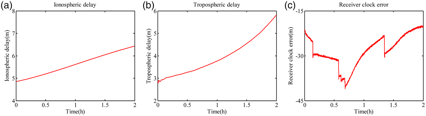
In the inertial aided wide-lane combination, the satellite clock error, receiver clock error, ionospheric delay and tropospheric delay are not eliminated. The satellite clock error can be removed with the precise satellite orbit. So the receiver clock error, ionospheric delay and tropospheric delay are analysed. The one-second dual-frequency GPS data was taken from ftp://cddis.gsfc.nasa.gov/pub/gps/data. In particular, data corresponding to the day 2014-01-07 taken from the IGS station of SHAO (Ashtech UZ12 receiver) are considered. The cut-off elevation angle is set at 15°. The sky plot of GPS is show in Figure 1.

Figure 1. Sky plots (azimuth vs. elevation).
The time series of the above three types of error is shown in Figure 2. The error differencing between two consecutive epochs in the time domain is given in Figure 3. The error series from Figure 2 and Figure 3 shows that the ionospheric delay and wet tropospheric delay varies slightly between two consecutive epochs (Zhang, Reference Zhang2007). The observation equation differencing between two consecutive epochs in the time domain can weaken both of the errors. In contrast, the receiver clock error fluctuates significantly in time. More data from multiple locations are used to analyse the variation of ionospheric delay, wet tropospheric delay and receiver clock error and all experience obtain the same result. In order to eliminate the receiver clock error in the inertial aided wide-lane combination, the differencing computation between two satellites is conducted. The inertial aided wide-lane combination DV (DV′ WL) is expressed as:
 $$DV^{\prime}_{{\rm WL}} = \Delta {{\it \Phi} ^{\prime}}_{{\rm WL}}^i - \Delta {{\it \Phi} ^{\prime}}_{{\rm WL}}^{{\rm base}} = \lambda _{{\rm 1, - 1}} \left( {b_1 - b_2} \right) + \delta \Delta M_{\it \Phi} + \delta \Delta \varepsilon _{\it \Phi} + \delta \Delta \varepsilon _{{\rm INS}} $$
where the superscript i indicates the ith satellite, the superscript base indicate the base satellite without cycle slip.

Figure 2. Error analysis: (a) ionospheric delay; (b) tropospheric delay; (c) receiver clock error.

Figure 3. Error variation (1s) analysis: (a) ionospheric delay; (b) tropospheric delay; (c) receiver clock error.
The standard deviation of DV GF, DV MW and DV′ WL are expressed as:
 $$\sigma _{{\rm GF}} = 2\sqrt {\sigma _{{M}_{\it \Phi}} ^2 + \sigma _{\varepsilon _{\it \Phi}} ^2} $$
 $$\sigma _{{\rm MW}} = \sqrt {2u_{1, - 1}^2 \sigma _{M_{\it \Phi}} ^2 + 2u_{1,1}^2 \sigma _{M_{P}} ^2 + 2u_{1, - 1}^2 \sigma _{\varepsilon _{\it \Phi}} ^2 + 2u_{1,1}^2 \sigma _{\varepsilon _{P}} ^2} $$
 $$\sigma ^{\prime}_{{\rm WL}} = 2\sqrt {u_{1, - 1}^2 \sigma _{M_{\it \Phi}} ^2 + u_{1, - 1}^2 \sigma _{\varepsilon _{\it \Phi}} ^2 + \sigma _{{\rm INS}}^2} $$
Compared with the DV
MW, the inertial aided DV is without the pseudorange multipath and pseudorange noise, while the INS position error is introduced. In the process to compare the σ
MW and
 ${\sigma^{\prime}_{{\rm WL}}} $
, the pseudorange multipath, pseudorange noise and INS error are the most important factors. Multipath effect is caused by the reflections of satellite signals from nearby objects, such as buildings, trees, vehicles and water. The multipath effect varies in different environments, so it is difficult to determine its variances. Typically, the maximum value of multipath is less than 1 m for pseudorange and less than 15 mm for carrier phase (Strang and Borre, Reference Strang and Borre1997). Though the work to determine the value of multipath effect is difficult, what is certain is that the pseudorange is more affected by multipath than carrier phase. So suppose the variance of multipath effect is one third of the maximum and the variances
${\sigma^{\prime}_{{\rm WL}}} $
, the pseudorange multipath, pseudorange noise and INS error are the most important factors. Multipath effect is caused by the reflections of satellite signals from nearby objects, such as buildings, trees, vehicles and water. The multipath effect varies in different environments, so it is difficult to determine its variances. Typically, the maximum value of multipath is less than 1 m for pseudorange and less than 15 mm for carrier phase (Strang and Borre, Reference Strang and Borre1997). Though the work to determine the value of multipath effect is difficult, what is certain is that the pseudorange is more affected by multipath than carrier phase. So suppose the variance of multipath effect is one third of the maximum and the variances
 $\sigma _{\varepsilon _{\it \Phi}} $
,
$\sigma _{\varepsilon _{\it \Phi}} $
,
 $\sigma _{\varepsilon _{P}} $
,
$\sigma _{\varepsilon _{P}} $
,
 $\sigma _{{M}_{\it \Phi}} $
and
$\sigma _{{M}_{\it \Phi}} $
and
 $\sigma _{{M}_{P}} $
are set as 5 mm, 200 mm, 5 mm and 300 mm. At the same time, the assumption that standard deviation of the multipath and noise are identical on both frequencies and considered uncorrelated is used. The detection accuracy of cycle slip for DV
MW and inertial aided DV is calculated by:
$\sigma _{{M}_{P}} $
are set as 5 mm, 200 mm, 5 mm and 300 mm. At the same time, the assumption that standard deviation of the multipath and noise are identical on both frequencies and considered uncorrelated is used. The detection accuracy of cycle slip for DV
MW and inertial aided DV is calculated by:
 $$\sigma _s = \displaystyle{\sigma \over {\lambda _{1, - 1}}} $$
where σ is the standard deviation of DV.
The INS position variance σ INS changes with different INS grade and self-navigation time. The accuracy of cycle slip for DV MW and inertial aided DV WL (DV′ WL) is computed and given in Figure 4. When the INS position error is less than 0·179 m, the DV′ WL has higher accuracy than DV MW.

Figure 4. Detection accuracy of cycle slip for DV MW and DV′ WL.
5. INERTIAL AIDED CYCLE SLIP DETECTION AND REPAIR
The cycle slip detection and repair algorithms are mathematically derived from testing statistical hypotheses. Cycle slip detection and repair are basically two different tasks. The first work of cycle slip detection is to know whether cycle slip occurs or not. The second step is the work to calculate the size of slip cycle for correction (Altmayer, Reference Altmayer2000).
The null hypothesis means no cycle slip occurred. The probability density function follows that of a Gaussian distribution. The mean value of the decision variable is zero and the standard deviation is σ, which is described:
 $$H_0 :DV \sim N\left( {0,\sigma} \right)$$
The alternative hypothesis means cycle slip follows the Gaussian distribution but is centred at b, with the standard deviation σ, which is described:
 $$H_1 :DV \sim N\left( {b,\sigma} \right)$$
where b is the number of cycle slips. When the decision variable is less than a certain threshold, the null hypothesis H 0 will be accepted, which implies no cycle slip is present, otherwise the alternative hypothesis H 1 will be accepted, which implies at least one cycle slip occurred.
The testing probabilities, such as probabilities of false alarm and missed detection are also derived from the statistical testing. The probabilities of false alarm and missed detection are shown in Figure 5. T D represents the chosen threshold for cycle slip detection. It can be seen that the probabilities of missed detection and false alarm are S1 and S2, respectively, with the standard deviation σ′WL. At the same time the probabilities of missed detection and false alarm are S1 + S3 and S2 + S4, respectively, if the standard deviation is equal to σ MW. The probability of false alarm and missed detection for the DV MW is more than these for DV′ WL. Compared with the Melbourne-Wübbena decision variable, the inertial aided decision variable has the higher accuracy. The analysis process of cycle determination is similar to cycle detection, which is not repeated here.

Figure 5. Probability of false alarm and missed detection.
Figure 6 shows the scheme of cycle slip detection and repair algorithm applied in the paper. The DV
GF with high accuracy is used to detect whether cycle slip exists. If DV
GF is less than the threshold T
D, there is no cycle slip in the carrier phase observation. Otherwise, the value of
 $\Delta {{\it \Phi} '}_{{\rm WL}} $
for base satellite without cycle slip and the ith satellite with cycle slip will be calculated. Then the inertial aided decision variable (DV
′
WL) is calculated. The cycle slip is identified and repaired with the value of DV
GF.
$\Delta {{\it \Phi} '}_{{\rm WL}} $
for base satellite without cycle slip and the ith satellite with cycle slip will be calculated. Then the inertial aided decision variable (DV
′
WL) is calculated. The cycle slip is identified and repaired with the value of DV
GF.

Figure 6. Cycle slip detection and repair.
According the above analysis, the DV GF has high accuracy. It is able to detect the position of cycle slip, but not to calculate the size of cycle slip alone. If the cycle slip cannot be calculated accurately, the ambiguity parameter will be re-initialised when the cycle slip occurs. The resolution method is the primary scheme subject to the unrepaired cycle slip in PPP/INS tightly coupled navigation. With the inertial aided DV, the cycle slip can be identified and repaired. The ambiguity parameter resolved in the last epoch will be regarded as the filter initial value for the next epoch, which is the new resolution scheme. The two resolution schemes are sketched in Figure 7.

Figure 7. Two process schemes for cycle slip.
6. FIELD TEST AND ANALYSIS
Field tests were conducted to evaluate the performance of the inertial aided cycle slip detection and repair method. The test system comprised two Leica GPS receivers and one navigation grade IMU. Raw IMU data and GPS data were collected throughout the test navigation. One of the Leica receivers was set up as a reference station and the other one was used as rover receiver with its antenna above the roof of the test vehicle. A set of dual-frequency observational GPS data with 1 s sampling interval was collected and 100 Hz INS data was received and stored in a book computer. The whole time of the test was about 20 minutes. The GPS observation was processed using the GPS software GrafNav™ 8·0 in Differential GPS (DGPS) mode and the solution was regarded as the position and velocity reference. The attitude reference was generated by the DGPS/INS integrated system using Inertial Explorer processing software, which promises much better accuracy than the proposed PPP/INS tightly coupled navigation system using precise point position mode. The specifications of the IMU are given in Table 1. The reference solution accuracy in these conditions is summarised in Table 2. The experienced trajectory is shown in Figure 8.

Figure 8. Field test trajectories.
Table 1. Navigation grade IMU technical data.
Table 2. Reference solution accuracy.

A self-navigation position accuracy of the INS used in the field test with PPP observation correction is given in Figure 9. The results show that the position can achieve an accuracy of 0·006 m, 0·055 m and 0·153 m for 1 s, 3 s and 5 s self-navigation time, respectively. According to the analysis result of Figure 2, the accuracy of cycle slip for DV′ WL is better than DV MW over less than 5 s self-navigation time. When the PPP/INS tightly coupled system is applied for the navigation work, the GPS sampling interval is usually less than 1 s in order to calculate the position of a high speed object accurately.

Figure 9. Inertial navigation system position accuracy.
In order to verify the efficiency of the inertial aided cycle slip detection and repair method, a length of observation without cycle slip is chosen. The value of DV GF, DV MW and DV′ WL are calculated and shown in Figure 10. The standard deviations (STD) of the DV are 0·002 m, 0·045 m and 0·010 mm, respectively. The STD of DV GF is the least of the above three values. The STD of DV′ WL is less than the STD of DV MW, which shows the inertial aided decision variable for cycle slip has higher accuracy than DV MW. In general, the cycle slip detection threshold is set less than a quarter of wavelength. The maximum value of DV MW reaches 0·243 m, which is more than a quarter of wavelength. So the DV MW will lead to large error, if it is used to detect the cycle slip. In addition, some receivers have much larger code noise, which may result in larger errors in DV MW.

Figure 10. Cycle slip decision variable without cycle slip.
For testing the case when cycle slip occurs on the carrier phase observations, a simulated small cycle slip ranging from one to six cycles have been added to the carrier phase observation. The simulated cycle slip values of L1 and L2 on PRN5 are shown in Table 3. The value of DV GF and DV′ WL with simulated small slip cycle on PRN5 is given in Figure 11. The values of DV GF and DV′ WL on the time of 373319 s, 373519 s, 373719 s and 373919 s are significantly greater than the other values, which can detect the position of cycle slip. The cycle slip repair result is summarised in Table 4 combining the value of DV GF and DV′ WL. This clearly illustrates that the new inertial aided method is very effective, and all the simulated small cycle slip is successfully identified.

Figure 11. Cycle slip decision variable with small cycle slip.
Table 3. Simulated small cycle slip on PRN5.
Table 4. Repair result for simulated small cycle slip.
In order to study the influence of small cycle slip on integrated navigation, the ambiguity result of PRN5 for the two schemes in Figure 7 are shown in Figure 12. The simulated cycle slip at the GPS time of 373719 s is left in the observation. The legend of scheme one represents the primary method which needs ambiguity re-initialisation and the legend of scheme two represents the method which can detect and repair the cycle slip. There is an obvious ambiguity initialisation process for scheme one in Figure 12.

Figure 12. Ambiguity resolution of PRN5 with small cycle slip.
Simulated large cycle slip ranging from 10 to 20 cycles has been added to the carrier phase observation at the same time. The simulated cycle slip values of L1 and L2 on PRN5 are shown in Table 5. The value of DV GF and DV′ WL with simulated large slip cycle on PRN5 is shown in Figure 13. The cycle slip repair result is summarised in Table 6. The same as the result for small cycle slip, the new inertial aided method is very effective in detecting and identifying the large cycle slip.

Figure 13. Cycle slip decision variable with large cycle slip.
Table 5. Simulated large cycle slip on PRN5.
Table 6. Repair result for simulated small cycle slip.
The simulated cycle slip at the GPS time of 373719 s is left in the observation. Figure 14 plots the ambiguity resolution series of PRN5. A position comparison of the two schemes is conducted in Figure 15. Table 7 illustrates Root Mean Square (RMS) and maximum value of position error for the data from 373919 s to 374119 s. There is an obvious ambiguity initialisation process for scheme one, which is the same as the small cycle slip situation. Figure 15 shows that scheme two, which can realise the repair of cycle slip, provides the better navigation results. The results show that the position of scheme two can achieve an accuracy of 0·039 m, 0·052 m and 0·308 m in the north, east and down coordinate components, respectively. Compared to scheme one, scheme two improves all the errors of position error in the north, east and down directions by 60%, 26% and 22% RMS, respectively. The three-dimensional position error for scheme one and scheme two is shown in Figure 16. Compared with the scheme one (0·415 m), the 3D position error from scheme two dropped down to 0·315 m. To further assess the effect of INS on the state covariance estimate, estimated variance of the position is shown in Figure 17, where the two schemes are the same as that in Figure 16. Figure 17 shows that the position accuracy in the north, east and down directions are improved by scheme two, especially at the time when the cycle slip occurs.

Figure 14. Ambiguity resolution of PRN5 with large cycle slip.

Figure 15. The position error for different schemes: (a) position error in north; (b) position error in east; (c) position error in down.

Figure 16. The three-dimensional position error for different schemes.

Figure 17. Kalman filter estimated position variances for different schemes: (a) position variances in north; (b) position variances in east; (c) position variances in down.
Table 7. Comparison of two schemes in terms of position error.

The roll, pitch and yaw errors of scheme one and scheme two are given in Table 8 and Figure 18. Compared with the scheme one, the scheme two improves all the errors of roll angles, pitch angles, and yaw angles by 2·6%, 2·4%, and 2·8% RMS, respectively. The improvement in the attitude is much less than the position, since the attitude estimation mainly relies on the Doppler measurements, which are without cycle slip.

Figure 18. The attitude error for different schemes: (a) attitude error in roll; (b) attitude error in pitch; (c) attitude error in yaw.
Table 8. Comparison of two schemes in terms of attitude error.
The influence of large cycle slip on several satellites is analysed. The three-dimensional position error for scheme one and scheme two is shown in Figure 19. The blue line and green line are the solution differences with respect to the reference value from scheme one, when the large cycle slip occurs on three and five satellites, respectively. The red line is the solution differences with respect to the reference value from scheme two. The navigation results of scheme two are the same as the situation when cycle slip occurs on three or five satellites. When large cycle slip occurs on several satellites, cycle slip is detected and repaired from scheme two, which is able to obtain better performance than scheme one.

Figure 19. The three-dimensional position error for different schemes.
7. CONCLUSION
This paper presents an inertial aided cycle slip detection and repair method applied in PPP/INS tightly coupled navigation to improve the accuracy of position, velocity and attitude parameters. Inertial information is used to construct the new wide-lane combination decision variable, which avoids the high noise and multipath from pseudorange.
Through the analysis and comparison of the error of traditional Melbourne-Wübbena decision variable and inertial aided decision variable, the critical value of INS position error which makes the new decision variable attain better performance is calculated. When the INS position error is less than the critical value, the inertial aided decision variable has higher accuracy than the DV MW.
Simulated small and large cycle slip are added to the carrier phase observation. The inertial aided method is very effective in detecting and repairing small and large cycle slips. The ambiguity re-initialisation method and cycle slip method are compared under large cycle slip situations. The inertial aided cycle slip detection and repair method can provide benefits in the accuracy of the navigation solution, compared to the ambiguity re-initialisation method.
FINANCIAL SUPPORT
The work is partially sponsored by the Fundamental Research Funds for the Central Universities (grant number: 2014ZDPY29) and partially sponsored by A Project Funded by the Priority Academic Program Development of Jiangsu Higher Education Institutions (grant number: SZBF2011-6-B35).