Introduction
Goosegrass is a troublesome weed in turfgrass and many cropping systems throughout the world (Holm et al. Reference Holm, Plucknett, Pancho and Herberger1977; Lee and Ngim Reference Lee and Ngim2000; Mueller et al. Reference Mueller, Barnett, Brosnan and Steckel2011; Takano et al. Reference Takano, Oliveira, Constantin, Braz and Padovese2016). Goosegrass is a diploid summer annual that can produce approximately 50,000 seeds with high (greater than 90%) viability potential (Chauhan and Johnson Reference Chauhan and Johnson2008; Jalaludin et al. Reference Jalaludin, Ngim, Bakar and Alias2010; Takano et al. Reference Takano, Oliveira, Constantin, Braz and Padovese2016).
Before the development of herbicides, farmers were required to understand a weed’s life cycle to develop proper management strategies. In the post-herbicide era, understanding a weed’s life cycle is pertinent due to multiple herbicide resistance (Van Acker Reference Van Acker2009). The development of herbicide resistance in goosegrass populations has been documented with dinitroanilines (Mudge et al. Reference Mudge, Gossett and Murphy1984), glyphosate (Lee and Ngim Reference Lee and Ngim2000), paraquat (Buker et al. Reference Buker, Steed and Stall2002), metribuzin plus MSMA (Brosnan et al. Reference Brosnan, Nishimoto and DeFrank2008), glufosinate-ammonium (Jalaludin et al. Reference Jalaludin, Ngim, Bakar and Alias2010), glufosinate plus paraquat (Seng et al. Reference Seng, Van Lun, San and Sahid2010), acetyl-CoA carboxylase inhibitors (McCullough et al. Reference McCullough, Yu, Raymer and Chen2016), and oxadiazon (McElroy et al. Reference McElroy, Head, Wehtje and Spak2017), and is suspected in several other populations. The development of herbicide resistance in weeds can be delayed with proper integration of cultural and chemical control practices (Van Acker Reference Van Acker2009).
Goosegrass germination begins in late winter or early spring and continues throughout the summer (Chauhan and Johnson Reference Chauhan and Johnson2008). A surge in late-summer germination may also occur as the residual effects of spring-applied PRE herbicides dissipate in the soil. Heavy rainfall during this period may also enhance goosegrass germination, further exacerbating late-summer infestations. The potential maturation of goosegrass plants establishing in late summer could warrant control by turf managers if viable seed is produced in the autumn.
Environmental cues impact the time a weedy species completes its life cycle; this, in turn, influences timing of control measures. There is an interaction of goosegrass growth stage on the efficacy of many herbicides used for POST control in turfgrass. Generally, most herbicides become less effective as goosegrass matures, and multiple applications may be required for control (Burke et al. Reference Burke, Wilcut and Porterfield2002; Corbett et al. Reference Corbett, Askew, Thomas and Wilcut2004). Studying the impact of reduced average weekly temperatures in the autumn on goosegrass development will lead to a better understanding about whether controlling plants with herbicides is needed before viable seed is produced. The study objective was to determine whether goosegrass seeds germinating on August 15 would complete a life cycle and produce viable seed before the first killing frost in Clemson, SC, typically November 15.
Materials and Methods
Goosegrass seeds were collected from a low maintenance turf site, the Cherry Farm at Clemson University (Clemson, SC) on October 25, 2016, and stored at 4 C. Seeds were sown in 1020 NCR trays (Landmark Plastic, Akron, OH, USA) filled with a sterile growing medium (Farfard® Growing Mix 3B, Sun Gro Horticulture Agawam, MA, USA). Trays were placed on a misting bench to promote germination for a period of 10 d, then relocated into a growth chamber (Controlled Environments, Hendersonville, NC, USA). Growth-chamber temperatures were maintained at the weekly temperature regime representing the 30-yr average (1986 to 2016) for Clemson, SC, beginning August 15 (Table 1; NOAA 2018). Once a minimum of 80 plants emerged and matured to the 2-leaf stage, seedlings were transplanted to 10 by 9 cm greenhouse pots (Landmark Plastic) filled with sterile growing medium (Farfard® Growing Mix 3B). Plants were maintained under a 14-h photoperiod and a light intensity of 500 µmol m−2 s−1 and subirrigated to prevent moisture stress. Plants were not clipped, and no supplemental nutrition was added throughout the experiment.
Table 1 Growth-chamber air temperature regime to simulate late-summer conditions in Clemson, SC.Footnote a

a Temperatures represent 30-yr weekly averages (1986–2016) from August 15 (Week 1) through December 5 (Week 16). The maximum temperature was maintained for 14 h, and the minimum temperature was maintained for 10 h. Plants were maintained under a 14-h photoperiod and a light intensity of 500 µmol m−2 s−1.
The experiment was arranged in a randomized complete block design, each block consisted of 20 goosegrass plants, for a total of 80 plants. Blocking was used to eliminate any spatial effect within the growth chamber. Two experimental runs were conducted, October to January 2016 to 2017 and 2017 to 2018. Plants were harvested at 7, 12, 19, 26, 33, 40, 47, 54, 61, and 68 d after emergence (DAE). On each sampling date, 1 plant was removed from each of the blocks. The stage of phenological development was noted and characterized based on the BBCH scale. As described by Hess et al. (Reference Hess, Barralis, Bleiholder, Buhr, Eggers, Hack and Stauss1997), the abbreviation “BBCH” derives from the institutes that jointly developed the scale: BBA, Biologische Bundesanstalt fur Land- und Forstwirtschaft (German Federal Biological Research Centre for Agriculture and Forestry); BSA, Bundessortenaml (German Federal Variety Authority); Chemical Industry, Industrieverband Agrar, IVA (German Association of Manufacturers of Agrochemical Products). Plant material was destructively harvested into plant parts to determine leaf dry weight (LDW), culm dry weight (CDW), root dry weight (RDW), and raceme dry weight (RaDW). Leaf, culm, and raceme material was rinsed with flowing water to remove soil and unwanted debris. Root material was washed in a basin with a combination of free-flowing water and sieves. Dissected rinsed plant material was then placed into paper bags and oven-dried at 80 C for 72 h. At the completion of the drying period, plant material was weighed to determine biomass. The root-to-shoot ratio was determined by dividing the RDW by the combined LDW, CDW, and RaDW (Oliveira et al. Reference Oliveira, Rodríguez-Soalleiro, Pérez-Cruzado, Cañellas, Sixto and Ceulemans2018).
To determine the quantity of seeds produced by each plant, the number of florets in 10 mm of the raceme was randomly sampled 25 times for each plant, and the average number was calculated; therefore, means were based on 100 samples. The average raceme length and total number of racemes for each plant were measured, and the number of seeds per plant was determined by extrapolating the number of florets in 10 mm by the total length of raceme per plant. At the completion of the life cycle, germination rates were determined in triplicate on petri dishes.
JMP Pro v. 13 (SAS Institute, Cary, NC, USA) was used for all statistical calculations and graphics. A logistic four-parameter growth curve was used to model the response of each variable (Yano et al. Reference Yano, Morisaki, Matsubara, Ito and Kitano2018). The terms in the model included: upper asymptote, lower asymptote, inflection point (i.e., point of maximum growth), and overall growth rate (Paine et al. Reference Paine, Marthews, Vogt, Purves, Rees, Hector and Turnbull2012). The equation used to model response variables is (Paine et al. Reference Paine, Marthews, Vogt, Purves, Rees, Hector and Turnbull2012):
 $$y{\equals}{{d{\minus}c} \over {[{\rm }1{\rm }{\plus}{\rm exp}\left( {{\minus}a{\rm }{\times}{\rm Time }{\minus}b} \right)]}}{\plus}\in{\rm }$$
Where y is the plant response of interest (e.g., LDW, CDW, RDW, RaDW, number of racemes, number of seeds per plant, root-to-shoot ratio, and total dry weight [TDW]), d is the upper bound of the y values, c is the lower bound of the y values, b is the inflection point of the growth of y over time, a is the growth rate, and ∈ is random error as outlined by Paine et al. (Reference Paine, Marthews, Vogt, Purves, Rees, Hector and Turnbull2012). Note that the reported adjusted growth rate for this nonlinear function is (Paine et al. Reference Paine, Marthews, Vogt, Purves, Rees, Hector and Turnbull2012):
 $${\rm \tau }{\equals}{{(d{\minus}c)(a)} \over 6}$$
Several parameters were estimated through logistic regression based on the biomass for leaf, culm, root, and raceme of individual goosegrass plants over time. These parameters included growth rate (both culm and leaf), inflection point, lower asymptote, upper asymptote, and R2 values (Table 2). The upper asymptote is the point of the growth curve that represents the maximum of the parameter measured. The lower asymptote is the point of the growth curve that represents the minimum of the parameter measured. The inflection point represents the DAE when exponential growth of the parameter measured occurs (Paine et al. Reference Paine, Marthews, Vogt, Purves, Rees, Hector and Turnbull2012).
Table 2 Goosegrass growth rate, inflection point, lower asymptote, upper asymptote, and R2 values for culm dry weight, leaf dry weight, number of racemes, number of seeds per plant, raceme dry weight, root dry weight, root-to-shoot ratio, and total dry weight estimated through logistic regression for growth models of goosegrass plants sampled at 7-d intervals for 68 d.Footnote a

a Plants grown in a controlled environment under late-summer simulated maximum and minimum temperatures for Clemson, SC. The maximum temperature was maintained for 14 h, and the minimum temperature was maintained for 10 h. Plants were maintained under a 14-h photoperiod and a light intensity of 500 µmol m−2 s−1. Two experimental runs with four replications were conducted: October to January 2016–2017 and 2017–2018.
b DAE, days after emergence.
Results and Discussion
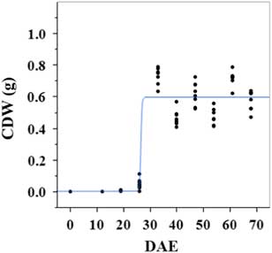
Estimated growth parameters for CDW were 0.46 g d−1, inflection point of 26.5 DAE, lower asymptote of 0.002 g, upper asymptote of 0.6 g, and an R2 value of 0.9 (Figure 1; Table 2). Estimated growth parameters for LDW were 0.39 g d−1, inflection point of 26.6 DAE, lower asymptote of 0.01 g, upper asymptote of 0.73 g, and an R2 value of 0.95 (Figure 2; Table 2). Culm and leaf growth experienced a similar trend, and at approximately 26 to 27 DAE, exponential growth occurred and the upper asymptote was reached.

Figure 1 Logistic regression of combined culm dry weight (CDW) and days after emergence (DAE) for two runs of a growth-chamber experiment under simulated autumn maximum and minimum temperatures. Ten sampling dates are represented, with 8 individual plants harvested on each date, n = 1 (refer to Equations 1 and 2 in text).
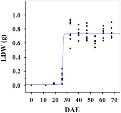
Figure 2 Logistic regression of combined leaf dry weight (LDW) and days after emergence (DAE) for two runs of a growth chamber experiment under simulated autumn maximum and minimum temperatures. Ten sampling dates are represented, with 8 individual plants harvested on each date, n = 1 (refer to Equations 1 and 2 in text).
In a greenhouse study, Takano et al. (Reference Takano, Oliveira, Constantin, Braz and Padovese2016) indicated the inflection point for goosegrass culm and leaf material occurred at 53 DAE. Takano et al. (Reference Takano, Oliveira, Constantin, Braz and Padovese2016) conducted the greenhouse experiment from May to September 2015 in Maringa, Brazil. Neither temperature nor light conditions within the greenhouse were provided. Damalas et al. (Reference Damalas, Koutroubas and Fotiadis2018) noted European field violet (Viola arvensis Murray) initiated flowering at 53 DAE, seed started to shed at 60 DAE, and the life cycle was considered complete at 100 DAE. Bakhshandeh et al. (Reference Bakhshandeh, Pirdashti and Gilani2018) noted rice (Oryza sativa L.) initiated flowering at 93 DAE, and the life cycle was considered completed at 107 DAE.
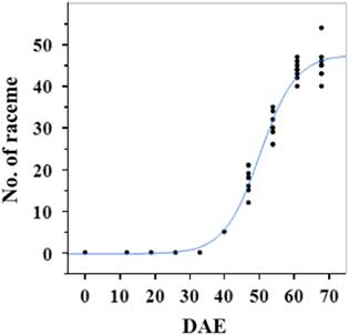
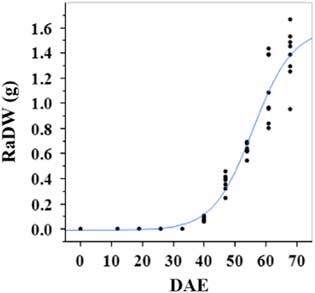
Estimated growth parameters for number of racemes were growth rate of 8 racemes d−1, inflection point of 50.3 DAE, lower asymptote of 0, upper asymptote of 47.6, and an R2 value of 0.99 (Figure 3; Table 2). Estimated growth parameters for number of seeds per plant were 317.4 seeds d−1, inflection point of 50.7 DAE, lower asymptote of 0, upper asymptote of 1901.2, and an R2 value of 0.97 (Figure 4; Table 2). Estimated growth parameters for RaDW (including germinable seed) were 0.04 g d−1, inflection point of 56.0 DAE, lower asymptote of 0.00 g, upper asymptote of 1.59 g, and an R2 value of 0.95 (Figure 5; Table 2). Racemes emerged at 26 DAE, indicating the initiation of reproductive growth (Table 3). Our model estimated that each plant would produce 1,901.2 seeds at the completion of its life cycle (Figure 4). Following seed production, it was determined in a separate petri-dish study that 33% of this seed could immediately germinate (unpublished data). The germination assay was performed in the greenhouse under natural light conditions and temperatures ranged from 21 to 26 C. Therefore, each goosegrass plant emerging during late summer in Clemson, SC, has the potential to produce approximately 630 new plants that season (if weather conditions are favorable for germination) or deposit this quantity of viable seed back into the soil seedbank. If the plants that produce the viable seeds have been exposed to herbicides and survive, there are also implications for the development of herbicide resistance. The viable seeds that are being deposited back into the soil seedbank could have developed resistance, and over time the resistant biotype will dominate the soil seedbank.
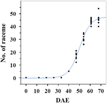
Figure 3 Logistic regression of combined number of raceme and days after emergence (DAE) for two runs of a growth chamber experiment under simulated autumn maximum and minimum temperatures. Ten sampling dates are represented, with 8 individual plants harvested on each date, n = 1 (refer to Equations 1 and 2 in text).

Figure 4 Logistic regression of combined number of seeds per plant and days after emergence (DAE) for two runs of a growth chamber experiment under simulated autumn maximum and minimum temperatures. Ten sampling dates are represented, with 8 individual plants harvested on each date, n = 1 (refer to Equations 1 and 2 in text).
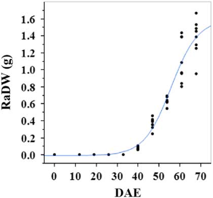
Figure 5 Logistic regression of combined raceme dry weight (RaDW) and days after emergence (DAE) for two runs of a growth chamber experiment under simulated autumn maximum and minimum temperatures. Ten sampling dates are represented, with 8 individual plants harvested on each date, n = 1 (refer to Equations 1 and 2 in text).
Table 3 Developmental stage of goosegrass on days after sowing (DAS) and days after emergence (DAE) with phenological development characterized on BBCH scale.Footnote a

a Goosegrass plants were sampled at 7-d intervals for 68 d, and phenological development was noted. Plants were grown in a controlled environment under late-summer simulated maximum and minimum temperatures for Clemson, SC. The maximum temperature was maintained for 14 h, and the minimum temperature was maintained for 10 h. Plants were maintained under a 14-h photoperiod and a light intensity of 500 µmol m−2 s−1. Two experimental runs with four replications were conducted: October to January 2016–2017 and 2017–2018.
b Abbreviation: BBCH scale as described by Hess et al. (Reference Hess, Barralis, Bleiholder, Buhr, Eggers, Hack and Stauss1997). See text for description.
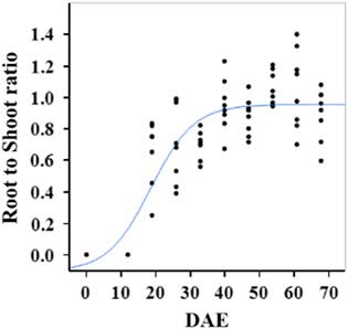
Estimated growth parameters for RDW were 0.04 g d−1, inflection point of 42.1 DAE, lower asymptote of 0.00 g, upper asymptote of 2.76 g, and an R2 value of 0.91 (Figure 6; Table 2). Estimated growth parameters for root-to-shoot ratio were 0.03 d−1, inflection point of 18.7 DAE, lower asymptote of 0, upper asymptote of 0.95, and an R2 value of 0.78 (Figure 7; Table 2). Estimated growth parameters for TDW were 0.98 g d−1, inflection point of 41.7 DAE, lower asymptote of 0.00 g, upper asymptote of 5.83 g, and an R2 value of 0.93 (Figure 8; Table 2).
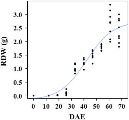
Figure 6 Logistic regression of combined root dry weight (RDW) and days after emergence (DAE) for two runs of a growth chamber experiment under simulated autumn maximum and minimum temperatures. Ten sampling dates are represented, with 8 individual plants harvested on each date, n = 1 (refer to Equations 1 and 2 in text).
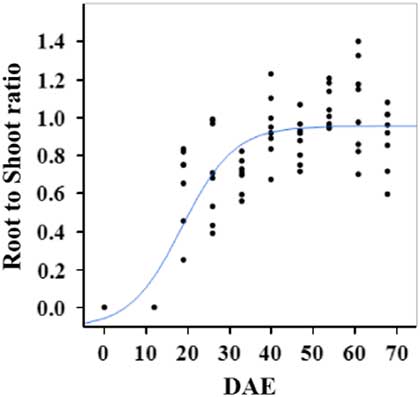
Figure 7 Logistic regression of combined root-to-shoot ratio and days after emergence (DAE) for two runs of a growth chamber experiment under simulated autumn maximum and minimum temperatures. Ten sampling dates are represented, with 8 individual plants harvested on each date, n = 1 (refer to Equations 1 and 2 in text).
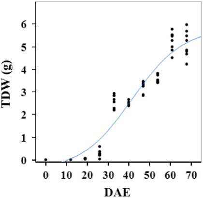
Figure 8 Logistic regression of combined total dry weight (TDW) and days after emergence (DAE) for two runs of a growth chamber experiment under simulated autumn maximum and minimum temperatures. Ten sampling dates are represented, with 8 individual plants harvested on each date, n = 1 (refer to Equations 1 and 2 in text).
Seedling emergence began 15 d after sowing (DAS); 2-leaf stage reached at 22 DAS; and, tillering commenced and 4-leaf stage reached at 27 DAS. At 34 DAS, 6-leaf stage was reached while at 41 DAS, 7-leaf stage, 4 to 5 tillers, and raceme initial emergence occurred. At 55 DAS, full raceme emergence and pollen was produced while at 62 DAS, 7 leaf, 8 to 9 tillers present started to mature, and leaf senescence began. Finally, seed began to shed at 76 DAS; and the life cycle was considered complete at 83 DAS (Table 3). Takano et al. (Reference Takano, Oliveira, Constantin, Braz and Padovese2016) reported goosegrass seedling emergence at 12 DAS; 2-leaf staged reached at 14 DAS while tillering commencement and 4-leaf staged reached at 21 DAS. At 41 DAS, 6- to 7-leaf stage was reached, tillering continued, and raceme emergence occurred. Pollen production and leaf senescence began at 50 DAS, while the life cycle was considered complete at 120 DAS.
Under controlled environmental conditions in the present study, goosegrass plants completed their life cycle in 83 DAS in comparison to 120 DAS in the greenhouse study by Takano et al. (Reference Takano, Oliveira, Constantin, Braz and Padovese2016). The reduction of 37 d could be due to lower maximum and minimum temperatures simulating autumn environmental conditions in Clemson, SC, or possible differences among biotypes used. Goosegrass germinating on approximately August 15 in Clemson, SC, will complete its life cycle and produce viable seed by approximately October 22, suggesting a need to control goosegrass plants emerging in late summer. However, this response should be evaluated under field conditions in Clemson, SC, and other locations in the southern United States.
Acknowledgments
No conflicts of interests have been declared. This research received no specific grant from any funding agency or the commercial or not-for-profit sectors.