


1. Introduction
The pioneering works of Mollo-Christensen (Reference Mollo-Christensen1963), Crow & Champagne (Reference Crow and Champagne1971), Moore (Reference Moore1977) and others have shown that the near field of turbulent jets comprises coherent structures which have inspired the recent development of reduced-order models for jet noise sources. The coherent structures were found to be fluctuations of a convected wave form, exhibiting the characteristics of amplification, saturation and decay. These instability waves, or wavepackets, arise due to the divergence of the jet which leads to a decay of downstream amplitudes. They have spatial extensions much larger than turbulence length scales and thus constitute a non-compact sound source, but are acoustically efficient due to their azimuthal coherence. It was not until recent times, however, that progress in numerical and experimental techniques allowed quantitative comparisons to be made between the near field of natural turbulent jets and various wavepacket models (Suzuki & Colonius Reference Suzuki and Colonius2006; Gudmundsson & Colonius Reference Gudmundsson and Colonius2011; Cavalieri et al. Reference Cavalieri, Rodríguez, Jordan, Colonius and Gervais2013). A consensus on how wavepacket structures in the jet relate to the far-field sound still remains elusive despite the great strides made in the methodology of predicting the acoustic field of jets. A description of the far-field sound in terms of such near-field structures is desirable for a more causal understanding of jet noise and the development of control strategies based on the physics of the flow.
From a theoretical perspective, wavepacket descriptions are useful since they capture certain aspects of jet turbulence and the radiated sound field, without recourse to equivalent source formulations and acoustic analogies such as those proposed by Lighthill (Reference Lighthill1952), Goldstein (Reference Goldstein2003) and Sinayoko, Agarwal & Hu (Reference Sinayoko, Agarwal and Hu2011). Wavepackets have thus been explored as a source mechanism (Crow & Champagne Reference Crow and Champagne1971; Michalke Reference Michalke1971; Crow Reference Crow1972) ever since the observation of coherent structures in jets.
Early attempts to model wavepackets using linear stability were often based on forced jets (e.g. Crighton & Gaster Reference Crighton and Gaster1976) or transitional jets with a laminar boundary layer at the jet nozzle (e.g. Laufer & Yen Reference Laufer and Yen1983) due to limitations of the available experimental equipment. In natural jets, the small amplitudes in the velocity field and the lack of a fixed phase reference made it difficult to draw conclusions about the nature of the source mechanism. Several important findings were nevertheless made, which are relevant to our present work. Azimuthally coherent wavepackets were found to be most clearly observed in the near pressure field of natural round jets, which is dominated only by a few low-order azimuthal modes (Michalke & Fuchs Reference Michalke and Fuchs1975; Armstrong, Michalke & Fuchs Reference Armstrong, Michalke and Fuchs1977; Fuchs & Michel Reference Fuchs and Michel1978). Michalke & Fuchs (Reference Michalke and Fuchs1975) also demonstrated that the two-point cross-spectral density (CSD) for any azimuthal mode depends only on the constituent of the pressure field for that azimuthal mode, which motivates azimuthally resolved analysis of wavepackets and source mechanisms.
Several early investigators such as Crighton & Gaster (Reference Crighton and Gaster1976) and Mankbadi & Liu (Reference Mankbadi and Liu1984) also observed that large-scale perturbations only constituted a small fraction of the total fluctuation energy. This led to the notion that, although high-Reynolds-number turbulent jets are characterized by the presence of small-scale structures across a wide range of wavenumbers and frequencies, as far as large-scale modes are concerned, turbulence establishes an equivalent base flow profile, and instability modes about this time-invariant base flow result in wavepackets. Crighton & Gaster (Reference Crighton and Gaster1976) extended parallel flow stability theory to the idealized mean flow of a slowly diverging turbulent jet by modelling these instability modes as linear perturbations. Due to linearization about a mean flow field which incorporates the results of Reynolds stresses, linear stability analysis of this form takes into account some of the inherent nonlinearities of the flow.
Recent works have built on these ideas to show that the pressure field near the jet flow can be characterized as superposed linear wavepackets of different azimuthal modes and frequencies. Suzuki & Colonius (Reference Suzuki and Colonius2006) used a quasi-parallel linear analysis and found reasonable agreement between the phase speed and growth rates predicted based on the measured mean flow field and those found experimentally, using a caged microphone array that measured azimuthally resolved pressure on a conical surface in the near acoustic field. Gudmundsson & Colonius (Reference Gudmundsson and Colonius2011) extended the analysis formally to consider the effect of a slowly diverging mean flow via a linear parabolized stability equation (LPSE) calculation, and investigated the extent to which pressure and velocity fluctuations in subsonic turbulent round jets can be described as linear perturbations to the mean flow field. By expanding the disturbances about the experimentally measured jet mean flow field, they found that linear models are useful for a statistical rendering of a wavepacket. Further corroborating the linear theory, Cavalieri et al. (Reference Cavalieri, Rodríguez, Jordan, Colonius and Gervais2013) found good agreement of LPSE solutions with time-resolved stereoscopic particle image velocimetry (PIV) in cross-stream planes up to the end of the potential core. Linear models have thus been shown to be particularly compelling due to the significant correlation of axisymmetric fluctuations in the jet with far-field sound and the close agreement between the near-field hydrodynamic amplitude and averaged phase predictions and experiments. An extensive review of wavepackets and turbulent jet noise is found in Jordan & Colonius (Reference Jordan and Colonius2013).
By contrast, far-field sound computation using linear wavepacket models is not as simple or as successful as the prediction of the near-field dynamics. The LPSE model appears to work well for supersonic jets, as shown by Sinha et al. (Reference Sinha, Rodríguez, Brès and Colonius2014), who found encouraging far-field sound results by using Kirchhoff surfaces to extend the near field obtained using the LPSE to the far field. However, for subsonic jets, LPSE models have largely been unsuccessful in predicting the sound field. One problem with the LPSE model is that since it does not yield the sound field directly, it is difficult to ascertain the reason behind this discrepancy. Combination of the LPSE model with a Kirchhoff-surface-based approach to predict the far-field sound is not straightforward as it is sensitive to the conditions of the model and the surface (Jordan & Colonius Reference Jordan and Colonius2013). Recent numerical simulations by Suponitsky, Sandham & Morfey (Reference Suponitsky, Sandham and Morfey2010) for low-Reynolds-number jets suggests that nonlinear interactions between instability waves can result in efficient sound radiators. However, the question of whether nonlinearity is equally important for high-Reynolds-number jets has never been adequately addressed. In this work, we present a linear model that gives the near-field hydrodynamics and produces a sound field directly in a single calculation using the linearized Euler equation (LEE). We show that the far-field sound pressure levels (SPLs) predicted are more than an order of magnitude smaller than the experimental results and investigate why this is the case through an investigation of two-point coherence in linear models such as LEE and experiments. The final model developed is not meant to be a predictive scheme but serves to explore the main missing feature of linear models related to this discrepancy.
This difference between experimental measurements and the sound field predicted can be understood through the effect of jitter (the randomness in the phase of wavepackets) on the amplitude of radiated sound in subsonic and supersonic jets. Although Ffowcs Williams & Kempton (Reference Ffowcs Williams and Kempton1978) found that, in general, jitter can increase the amplitude of radiated sound, Cavalieri et al. (Reference Cavalieri, Jordan, Agarwal and Gervais2011) showed that this has a significant effect in subsonic jets and only a minor influence in supersonic ones. This explains why the LPSE implementation used by Sinha et al. (Reference Sinha, Rodríguez, Brès and Colonius2014) did not encounter this problem. In subsonic turbulent jets, the flow fluctuations are not periodic, and randomness in the phase is associated with a coherence decay with distance, whereas in linear wavepacket models such as the ones developed in LEE computations, the fluctuations are time-periodic, and the coherence is exactly equal to unity. Using this observation, Cavalieri & Agarwal (Reference Cavalieri and Agarwal2014) showed that agreement in averaged near-field amplitudes and phases of a statistical source, which would be obtained by linear wavepacket models, is not a sufficient condition for a good agreement of the far-field sound. The sufficient condition is found to also require a match in the coherence function of the flow fluctuations, which is defined as the normalized CSD between two points in the jet. While matching the coherence between every two-point combination in a model with that found in physical jets is not trivial, for a line source such an operation is feasible. This is shown in a model problem in Cavalieri & Agarwal (Reference Cavalieri and Agarwal2014), which proves useful for the present work.
In §§ 2 and 3, we investigate how wavepackets in subsonic jets radiate sound by a direct axisymmetric computation using LEE, which leads to both the near-field hydrodynamics and the radiated sound, allowing us to relax some of the assumptions made in LPSE. We focus on the range of Strouhal numbers
 $0.3\leqslant \mathit{St}\leqslant 0.7$
at which peak noise occurs for polar angles less than 40° (Cavalieri et al.
Reference Cavalieri, Jordan, Colonius and Gervais2012). The computation is based on the mean flows measured by Cavalieri et al. (Reference Cavalieri, Rodríguez, Jordan, Colonius and Gervais2013), and the near-field and far-field results are compared with azimuthally resolved data from experiments (Breakey et al.
Reference Breakey, Jordan, Cavalieri, Léon, Zhang, Lehnasch, Colonius and Rodrıguez2013; Cavalieri et al.
Reference Cavalieri, Rodríguez, Jordan, Colonius and Gervais2013). The effect of coherence decay on the radiated sound is then studied in § 4 by imposing the experimentally obtained coherence data from Breakey et al. (Reference Breakey, Jordan, Cavalieri, Léon, Zhang, Lehnasch, Colonius and Rodrıguez2013) on the CSD of the near-field pressure from LEE at control surfaces enclosing the jet flow. Two surface types are explored: cylindrical surfaces that intersect the axisymmetric plane at a line parallel to the jet axis and conical surfaces that intersect the axisymmetric plane at a line sloping away from the jet axis with a positive nozzle–plane intercept. Since the CSD of the axisymmetric mode depends only on the axisymmetric component of the pressure field (see appendix A), application of the measured two-point coherence along the intersection lines is sufficient to match the coherence on these enclosing surfaces. The far-field sound is calculated using boundary value formulations based on the linear wave equation, as developed by Freund (Reference Freund2001) for cylindrical surfaces and Reba, Narayanan & Colonius (Reference Reba, Narayanan and Colonius2010) for conical surfaces. Sections 5 and 6 include further analysis of the role of coherence matching on the near-field hydrodynamics and the location of the surfaces on which this is applied. The objective is to investigate whether matching the near-field coherence profile in this manner improves the far-field SPL agreement with experimental results. This will indicate whether coherence is indeed the main missing feature in relating the far-field sound of turbulent subsonic jets to near-field fluctuations in linear wavepacket models.
$0.3\leqslant \mathit{St}\leqslant 0.7$
at which peak noise occurs for polar angles less than 40° (Cavalieri et al.
Reference Cavalieri, Jordan, Colonius and Gervais2012). The computation is based on the mean flows measured by Cavalieri et al. (Reference Cavalieri, Rodríguez, Jordan, Colonius and Gervais2013), and the near-field and far-field results are compared with azimuthally resolved data from experiments (Breakey et al.
Reference Breakey, Jordan, Cavalieri, Léon, Zhang, Lehnasch, Colonius and Rodrıguez2013; Cavalieri et al.
Reference Cavalieri, Rodríguez, Jordan, Colonius and Gervais2013). The effect of coherence decay on the radiated sound is then studied in § 4 by imposing the experimentally obtained coherence data from Breakey et al. (Reference Breakey, Jordan, Cavalieri, Léon, Zhang, Lehnasch, Colonius and Rodrıguez2013) on the CSD of the near-field pressure from LEE at control surfaces enclosing the jet flow. Two surface types are explored: cylindrical surfaces that intersect the axisymmetric plane at a line parallel to the jet axis and conical surfaces that intersect the axisymmetric plane at a line sloping away from the jet axis with a positive nozzle–plane intercept. Since the CSD of the axisymmetric mode depends only on the axisymmetric component of the pressure field (see appendix A), application of the measured two-point coherence along the intersection lines is sufficient to match the coherence on these enclosing surfaces. The far-field sound is calculated using boundary value formulations based on the linear wave equation, as developed by Freund (Reference Freund2001) for cylindrical surfaces and Reba, Narayanan & Colonius (Reference Reba, Narayanan and Colonius2010) for conical surfaces. Sections 5 and 6 include further analysis of the role of coherence matching on the near-field hydrodynamics and the location of the surfaces on which this is applied. The objective is to investigate whether matching the near-field coherence profile in this manner improves the far-field SPL agreement with experimental results. This will indicate whether coherence is indeed the main missing feature in relating the far-field sound of turbulent subsonic jets to near-field fluctuations in linear wavepacket models.
2. Numerical simulation with a fluctuating inflow boundary condition
The numerical set-up involves first solving the axisymmetric LEE for turbulent jets of speed Mach 0.4 and 0.6, whose mean velocity profiles are obtained from the experimental results of Cavalieri et al. (Reference Cavalieri, Rodríguez, Jordan, Colonius and Gervais2013). Based on unforced natural jets, these experiments were guided by the earlier experiments of Cavalieri et al. (Reference Cavalieri, Jordan, Colonius and Gervais2012), where it was determined that downstream superdirective radiation was predominantly due to the axisymmetric mode. Normalized quantities are used throughout the computation. Thus, in this section and the ones that follow, unless denoted by a tilde, e.g.
 $\tilde{q}$
, all variables
$\tilde{q}$
, all variables
 $q$
represent quantities normalized by using the jet diameter
$q$
represent quantities normalized by using the jet diameter
 $\tilde{D}$
, jet exit speed
$\tilde{D}$
, jet exit speed
 $\tilde{U} _{j}$
and ambient density
$\tilde{U} _{j}$
and ambient density
 $\tilde{{\it\rho}}_{\infty }$
as the length, velocity and density scales respectively.
$\tilde{{\it\rho}}_{\infty }$
as the length, velocity and density scales respectively.
The LEE is solved for the cases being investigated using a finite-difference solver (Dieste & Gabard Reference Dieste and Gabard2009), in which the spatial derivatives are approximated using a seven-point fourth-order dispersion-relation-preserving (DRP) scheme (Tam & Webb Reference Tam and Webb1993), which is optimized to minimize the dispersion error. A six-stage optimized explicit Runge–Kutta scheme is implemented to perform the time integration. The simulation domain is divided into six overlapping blocks which are synchronized between the stages of the Runge–Kutta scheme using message passing interfaces (MPIs). The time step is specified using a Courant–Friedrichs–Lewy (CFL) number of 1.2, and non-dimensional variables are used as input.
2.1. Adapting turbulent base flows for LEE
The turbulent base flows in Cavalieri et al. (Reference Cavalieri, Rodríguez, Jordan, Colonius and Gervais2013) were obtained using measurements from a traversing Pitot tube. Mean-flow measurements were subsequently interpolated to cylindrical coordinates based on numerical fits developed by Rodrıguez et al. (Reference Rodrıguez, Sinha, Bres and Colonius2013) and adapted to a grid suitable for LPSE. The results thus available consist of
 $95\times 351$
velocity vectors between
$95\times 351$
velocity vectors between
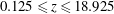 $0.125\leqslant z\leqslant 18.925$
and
$0.125\leqslant z\leqslant 18.925$
and
 $0.008\leqslant r\leqslant 5$
, where
$0.008\leqslant r\leqslant 5$
, where
 $z$
and
$z$
and
 $r$
are axial and radial distances respectively. The maximum grid separations of these data are
$r$
are axial and radial distances respectively. The maximum grid separations of these data are
 $({\rm\Delta}z)_{max}=0.2$
and
$({\rm\Delta}z)_{max}=0.2$
and
 $({\rm\Delta}r)_{max}=0.0389$
. In order to obtain results at a higher spatial resolution, and to ensure that directivity comparisons of the far-field SPLs can be made at a distance of 35 jet diameters (
$({\rm\Delta}r)_{max}=0.0389$
. In order to obtain results at a higher spatial resolution, and to ensure that directivity comparisons of the far-field SPLs can be made at a distance of 35 jet diameters (
 $D$
), it is required to first interpolate the data to a finer grid and then extrapolate the data in both the axial and radial directions such that the domain exceeds a distance of
$D$
), it is required to first interpolate the data to a finer grid and then extrapolate the data in both the axial and radial directions such that the domain exceeds a distance of
 $35D$
from the origin at polar angles between 0° and 90°. Furthermore, since the local density and pressure distributions corresponding to the base flow are not readily available from the experiments, they must be estimated from the velocity profiles based on some reasonable assumptions.
$35D$
from the origin at polar angles between 0° and 90°. Furthermore, since the local density and pressure distributions corresponding to the base flow are not readily available from the experiments, they must be estimated from the velocity profiles based on some reasonable assumptions.
In order to interpolate the data to a finer grid from the coarse experimental grid, a bivariate spline is used over a rectangular mesh. To extend the experimental data cross-stream, an exponentially decaying function is used such that the profiles are continuous in the radial direction. In the turbulent jets used, for
 $z\leqslant 18.925$
, the mean axial velocity decays to nearly zero as
$z\leqslant 18.925$
, the mean axial velocity decays to nearly zero as
 $r\rightarrow 5$
, so a simple exponential function with gradient matching at
$r\rightarrow 5$
, so a simple exponential function with gradient matching at
 $r=5$
suffices to give a smooth radial profile.
$r=5$
suffices to give a smooth radial profile.
To extrapolate the axial velocity data downstream, however, more attention is required as the profile both decays and spreads. Assuming a linear spread rate, a self-similarity profile is used as described by Pope (Reference Pope2000). Linear regression is applied to
 $1/\bar{u}(z,0)$
, the inverse of the normalized mean axial velocity along the jet centreline, between
$1/\bar{u}(z,0)$
, the inverse of the normalized mean axial velocity along the jet centreline, between
 $17.158\leqslant z\leqslant 18.925$
(which corresponds to the last 40 grid points in the finer grid) where its profile is nearly linear. The axial velocity along the jet centreline can thus be extrapolated using
$17.158\leqslant z\leqslant 18.925$
(which corresponds to the last 40 grid points in the finer grid) where its profile is nearly linear. The axial velocity along the jet centreline can thus be extrapolated using
 $$\begin{eqnarray}\frac{1}{\bar{u}(z,0)}=\frac{\tilde{U} _{j}}{\tilde{u} (z,0)}=\frac{1}{B}(z-z_{0}),\end{eqnarray}$$
where
 $z_{0}$
and
$z_{0}$
and
 $B$
are constants determined from linear regression. The axial variation of
$B$
are constants determined from linear regression. The axial variation of
 $1/\bar{u}(z,0)$
and the best-fit line obtained for the linear trailing section for the Mach 0.4 turbulent jet are shown in figure 1(a), and the extrapolated mean centreline axial velocity,
$1/\bar{u}(z,0)$
and the best-fit line obtained for the linear trailing section for the Mach 0.4 turbulent jet are shown in figure 1(a), and the extrapolated mean centreline axial velocity,
 $\bar{u}(z,0)$
, is shown in figure 1(b).
$\bar{u}(z,0)$
, is shown in figure 1(b).

Figure 1. For the Mach 0.4 turbulent jet: (a) linear regression on the trailing linear section of
 $1/\bar{u}(z,0)$
, (b) centreline axial velocity
$1/\bar{u}(z,0)$
, (b) centreline axial velocity
 $\bar{u}(z,0)$
extrapolated beyond
$\bar{u}(z,0)$
extrapolated beyond
 $z=18.925$
.
$z=18.925$
.
For the self-similar velocity profile along the radial direction, the cross-stream similarity variable was taken as
 $$\begin{eqnarray}{\it\eta}=\frac{r}{z-z_{0}}.\end{eqnarray}$$
The self-similar mean velocity profile is thus defined by
 $$\begin{eqnarray}f({\it\eta})=\frac{\bar{u}(z,r)}{\bar{u}(z,0)}.\end{eqnarray}$$
This is shown for the Mach 0.4 turbulent jet in figure 2(a), and a contour plot of the mean axial velocity plot is shown in figure 2(b). The mean radial velocity,
 $\bar{v}$
, is assumed to be zero as the radial velocity obtained from experiment had a lower order of magnitude than the axial velocity and is therefore assumed to have had negligible effect on the near-field structures and the radiated sound field; the results in § 3 confirm this hypothesis.
$\bar{v}$
, is assumed to be zero as the radial velocity obtained from experiment had a lower order of magnitude than the axial velocity and is therefore assumed to have had negligible effect on the near-field structures and the radiated sound field; the results in § 3 confirm this hypothesis.

Figure 2. For the Mach 0.4 turbulent jet: (a) self-similar radial profile of the mean axial velocity and its match at
 $z=43.1$
, (b) mean axial velocity
$z=43.1$
, (b) mean axial velocity
 $\bar{u}$
adapted for the LEE solver.
$\bar{u}$
adapted for the LEE solver.
2.2. Derivation of mean density, momentum and pressure using Crocco–Busemann relations
Although the experimental data of Cavalieri et al. (Reference Cavalieri, Rodríguez, Jordan, Colonius and Gervais2013) provided the mean velocity fields associated with the turbulent base flows, to incorporate the base flows in the LEE solver, it was necessary to derive the corresponding mean density, pressure and momenta. This is achieved using the Crocco–Busemann relation for the local mean density distribution of a round jet, which can be written as in Agarwal, Morris & Mani (Reference Agarwal, Morris and Mani2004):
 $$\begin{eqnarray}\frac{1}{\tilde{\bar{{\it\rho}}}(z,r)}=-\frac{1}{2}\frac{{\it\gamma}-1}{{\it\gamma}\tilde{\bar{p}}}(\tilde{\bar{u}}(z,r)-\tilde{U_{j}})\tilde{\bar{u}}(z,r)+\frac{1}{\tilde{{\it\rho}_{j}}}\frac{\tilde{\bar{u}}(z,r)}{\tilde{U_{j}}}+\frac{1}{\tilde{{\it\rho}}_{\infty }}\frac{\tilde{U_{j}}-\tilde{\bar{u}}(z,r)}{\tilde{U_{j}}}.\end{eqnarray}$$
Here,
 $\tilde{\bar{p}}=101\,325~\text{Pa}$
is the standard atmospheric pressure, and the far-field density,
$\tilde{\bar{p}}=101\,325~\text{Pa}$
is the standard atmospheric pressure, and the far-field density,
 $\tilde{{\it\rho}}_{\infty }=1.225~\text{kg}~\text{m}^{-3}$
, is equal to the ambient density of air at room temperature and atmospheric pressure. Assuming that the density at the jet exit,
$\tilde{{\it\rho}}_{\infty }=1.225~\text{kg}~\text{m}^{-3}$
, is equal to the ambient density of air at room temperature and atmospheric pressure. Assuming that the density at the jet exit,
 $\tilde{{\it\rho}}_{j}$
, is the same as the far-field ambient density,
$\tilde{{\it\rho}}_{j}$
, is the same as the far-field ambient density,
 $\tilde{{\it\rho}}_{\infty }$
(i.e. assuming constant static pressure and that the jet is at ambient temperature), equation (2.4) is simplified to
$\tilde{{\it\rho}}_{\infty }$
(i.e. assuming constant static pressure and that the jet is at ambient temperature), equation (2.4) is simplified to
 $$\begin{eqnarray}\tilde{\bar{{\it\rho}}}(z,r)=\left(-\frac{1}{2}\frac{{\it\gamma}-1}{{\it\gamma}\tilde{\bar{p}}}(\tilde{\bar{u}}(z,r)-\tilde{U_{j}})\tilde{\bar{u}}(z,r)+\frac{1}{\tilde{{\it\rho}}_{\infty }}\right)^{-1}.\end{eqnarray}$$
This is normalized by the jet exit density to give the non-dimensional density,
 $\bar{{\it\rho}}(z,r)=\tilde{{\it\rho}}(z,r)/\tilde{{\it\rho}}_{j}$
. The non-dimensional mean axial and radial momenta are then computed as
$\bar{{\it\rho}}(z,r)=\tilde{{\it\rho}}(z,r)/\tilde{{\it\rho}}_{j}$
. The non-dimensional mean axial and radial momenta are then computed as
 $\bar{{\it\rho}}\bar{u}$
and
$\bar{{\it\rho}}\bar{u}$
and
 $\bar{{\it\rho}}\bar{v}$
respectively. The mean density and axial momentum thus derived are shown for the Mach 0.4 turbulent jet in figure 3(a,b). It should be noted that the mean radial momentum is zero as the mean radial velocity has been assumed to be negligible. The non-dimensional mean pressure is assumed to be constant and is defined using the ambient pressure
$\bar{{\it\rho}}\bar{v}$
respectively. The mean density and axial momentum thus derived are shown for the Mach 0.4 turbulent jet in figure 3(a,b). It should be noted that the mean radial momentum is zero as the mean radial velocity has been assumed to be negligible. The non-dimensional mean pressure is assumed to be constant and is defined using the ambient pressure
 $\tilde{\bar{p}}$
and the jet exit velocity and density as
$\tilde{\bar{p}}$
and the jet exit velocity and density as
 $$\begin{eqnarray}\bar{p}(z,r)=\frac{\tilde{\bar{p}}}{\tilde{{\it\rho}}_{j}\tilde{U} _{j}^{2}}.\end{eqnarray}$$
The same procedure is carried out to adapt the base flow of the Mach 0.6 jet for the LEE solver.

Figure 3. For the Mach 0.4 turbulent jet: (a) mean density
 $\bar{{\it\rho}}$
, (b) mean axial momentum
$\bar{{\it\rho}}$
, (b) mean axial momentum
 $(\bar{{\it\rho}u})$
.
$(\bar{{\it\rho}u})$
.
2.3. Fluctuating inflow boundary condition
Since linearity allows separate computations for each frequency and azimuthal mode, we are able to focus on the axisymmetric mode, which is known to dominate the sound field at low polar angles (Cavalieri et al. Reference Cavalieri, Jordan, Colonius and Gervais2012). At larger polar angles, higher-order azimuthal modes are known to contribute to the sound field, but this is not the focus of the present work. To introduce axisymmetric linear instability waves into the jet, we modify the LEE solver with a fluctuating inflow boundary condition to match the frequency corresponding to the most energetic axisymmetric mode. This work is inspired by that of Bodony & Jambunathan (Reference Bodony and Jambunathan2012), who used an inflow boundary condition to perturb a high-speed mixing layer with spatial instability waves in order to investigate the effect of heating on the acoustic field radiated. However, any approach of perturbing a jet with linear instability waves in this manner must overcome two key obstacles. First, the linear instability waves introduced at the inflow must be able to pass through any upstream buffer zones, which are typically used to implement artificial boundary conditions that emulate an infinite computational domain by damping outgoing waves. Second, it needs to be ensured that the boundary condition does not generate sound on its own.

Figure 4. Computational set-up for generating the near field using LEE (not to scale).
One intuitive way to implement the inflow boundary condition would be to place momentum sources along the upstream boundary, which gives a resulting behaviour similar to that of a piston vibrating along the streamwise direction. However, this is incompatible with the buffer zone in place, which has similar features to that used by Dieste & Gabard (Reference Dieste and Gabard2009). Along the grid points on the buffer zone, the amplitude of characteristic waves travelling into the simulation domain,
 $q_{a}^{-}$
, is scaled by a factor
$q_{a}^{-}$
, is scaled by a factor
 ${\it\alpha}$
decreasing from 1 to 0:
${\it\alpha}$
decreasing from 1 to 0:
 $q_{a}^{-}(1-{\it\alpha})$
, where
$q_{a}^{-}(1-{\it\alpha})$
, where
 ${\it\alpha}$
varies as a simple cosine function along
${\it\alpha}$
varies as a simple cosine function along
 $z$
. This means that the amplitude of the characteristic wave travelling into the domain is set to zero at the boundary of the computational domain. Therefore, to implement momentum sources, it was required to increment the upstream boundary axial and radial momenta at each time step instead of setting them to prescribed values. The required instantaneous momenta are derived from the LPSE results for axial and radial velocities near the nozzle exit. These are given below with primes representing perturbation values and hats denoting complex variables:
$z$
. This means that the amplitude of the characteristic wave travelling into the domain is set to zero at the boundary of the computational domain. Therefore, to implement momentum sources, it was required to increment the upstream boundary axial and radial momenta at each time step instead of setting them to prescribed values. The required instantaneous momenta are derived from the LPSE results for axial and radial velocities near the nozzle exit. These are given below with primes representing perturbation values and hats denoting complex variables:
 $$\begin{eqnarray}\displaystyle & ({\it\rho}u)_{boundary}^{\prime }=\text{Re}\{(\bar{{\it\rho}}\hat{u} ^{\prime }+\hat{{\it\rho}}^{\prime }\bar{u})\text{e}^{\text{i}{\it\omega}t}\}, & \displaystyle\end{eqnarray}$$
 $$\begin{eqnarray}\displaystyle & ({\it\rho}v)_{boundary}^{\prime }=\text{Re}\{(\bar{{\it\rho}}\hat{v}^{\prime }+\hat{{\it\rho}}^{\prime }\bar{v})\text{e}^{\text{i}{\it\omega}t}\}. & \displaystyle\end{eqnarray}$$
However, such a boundary condition produces acoustic waves as well as instability waves, which makes it difficult to isolate the noise propagated from wavepackets formed in the jet. To get around this obstacle, a parallel flow section was added upstream of the jet nozzle, and the upstream buffer zone was extended to apply to the entire parallel flow region, as shown in the schematic in figure 4. The fluctuating boundary condition was applied to the boundary upstream of the parallel section. It was found that parallel flow sections of streamwise length greater than double the wavelength of the acoustic waves,
 $l>2{\it\lambda}$
, damp out the acoustic waves from the inflow boundary but allow linear instability waves to pass through. This is due to the fact that the parallel section exponentially amplifies instability waves introduced by the fluctuating boundary condition as they travel downstream, which overcomes the cosine damping of the buffer region. The amplitude of the instability wave at the jet nozzle is not particularly important as linearity allows us to scale results by matching the amplitude with experimental results at an axial station close to the jet nozzle in the same manner as done by Cavalieri et al. (Reference Cavalieri, Rodríguez, Jordan, Colonius and Gervais2013) for LPSE.
$l>2{\it\lambda}$
, damp out the acoustic waves from the inflow boundary but allow linear instability waves to pass through. This is due to the fact that the parallel section exponentially amplifies instability waves introduced by the fluctuating boundary condition as they travel downstream, which overcomes the cosine damping of the buffer region. The amplitude of the instability wave at the jet nozzle is not particularly important as linearity allows us to scale results by matching the amplitude with experimental results at an axial station close to the jet nozzle in the same manner as done by Cavalieri et al. (Reference Cavalieri, Rodríguez, Jordan, Colonius and Gervais2013) for LPSE.

Figure 5. Radiated pressure fields obtained by applying the fluctuating boundary condition on the Mach 0.4 turbulent jet base flow at (a)
 $\mathit{St}=0.3$
, (b)
$\mathit{St}=0.3$
, (b)
 $\mathit{St}=0.5$
and (c)
$\mathit{St}=0.5$
and (c)
 $\mathit{St}=0.7$
.
$\mathit{St}=0.7$
.

Figure 6. Radiated pressure field obtained by applying the fluctuating boundary condition on the Mach 0.6 turbulent jet base flow at (a)
 $\mathit{St}=0.3$
, (b)
$\mathit{St}=0.3$
, (b)
 $\mathit{St}=0.5$
and (c)
$\mathit{St}=0.5$
and (c)
 $\mathit{St}=0.7$
.
$\mathit{St}=0.7$
.
Numerical simulations using this set-up are carried out for the Mach 0.4 and 0.6 jets for Strouhal numbers of 0.3 to 0.7. The resulting pressure distributions, comparison of centreline axial velocity and the radial profile of axial velocity are shown in § 3.
3. Near-field wavepacket structure and far-field sound from LEE
The instantaneous radiated pressure fields obtained by implementing the inflow boundary condition on the Mach 0.4 turbulent jet for Strouhal numbers of 0.3, 0.5 and 0.7 are shown in figure 5(a)–(c) respectively. The same is shown for the Mach 0.6 turbulent jet in figure 6. All of these results are obtained after the initial transient phase during which spurious waves develop and exit the computational domain. The steady-state solution is achieved when the near- and far-field solutions have become periodic and only involves the single frequency at which the flow is excited using the inflow boundary condition. A wavepacket structure appears to be present in all cases immediately downstream of the jet nozzle and in the potential core region. It is also evident that acoustic waves are radiated to the far field. The magnitude and directivity of this sound field are compared with experimental data in § 3.4. It should be noted that the contour levels for figures 5 and 6 have been arbitrarily chosen to display the near- and far-field structures, and they are not representative of the actual amplitudes of the radiated pressure in any way.
3.1. Comparison between velocity fluctuations on the jet centreline obtained from LEE, LPSE and experiment
To determine the velocity fluctuations from LEE, the power spectral density (PSD) of the axial velocity data was computed for the final 20 periods of the simulations, when the transient effects become negligible and the simulation can be considered as periodic in time. As discussed earlier, the linear solutions have a free amplitude, which can be adjusted using the velocity spectra on the jet centreline. The free constant used to multiply the LEE amplitudes was chosen by matching amplitudes at a single point
 $(z,r)=(2,0)$
with experimental data in the same manner as done by Cavalieri et al. (Reference Cavalieri, Rodríguez, Jordan, Colonius and Gervais2013) for LPSE. Figure 7 shows comparisons between LEE, LPSE and experiment of the axial velocity fluctuations for the Mach 0.4 jet at Strouhal numbers between 0.3 and 0.7.
$(z,r)=(2,0)$
with experimental data in the same manner as done by Cavalieri et al. (Reference Cavalieri, Rodríguez, Jordan, Colonius and Gervais2013) for LPSE. Figure 7 shows comparisons between LEE, LPSE and experiment of the axial velocity fluctuations for the Mach 0.4 jet at Strouhal numbers between 0.3 and 0.7.

Figure 7. Comparison between LEE (blue lines), LPSE (grey dashed lines) and experimental velocity fluctuations (red dots) on the centreline for the Mach 0.4 jet. Panels (a)–(e) refer respectively to Strouhal numbers from 0.3 to 0.7 with increments of 0.1.
There is an amplification of four orders of magnitude of the fluctuation energy in the experiment between the nozzle and the end of the potential core (
 $z\approx 5$
–5.5), and, in this region, close agreement is observed between LEE, LPSE and experimental results. However, downstream of the potential core end, LEE underpredicts the experimental velocity fluctuations, but the agreement with experimental results is better than that found using LPSE. Apart from Cavalieri et al. (Reference Cavalieri, Rodríguez, Jordan, Colonius and Gervais2013), this behaviour was also observed by Suzuki & Colonius (Reference Suzuki and Colonius2006) and Gudmundsson & Colonius (Reference Gudmundsson and Colonius2011), who attributed this discrepancy to fluctuations that were uncorrelated with upstream instability waves. These authors noted that the application of proper orthogonal decomposition (POD) on the pressure fluctuations to obtain modes correlated axially, and use of the first POD modes, allowed uncorrelated fluctuations to be filtered out and significantly improved agreement at downstream positions. However, since the experimental results included here were obtained from single-point hot-wire measurements, the POD filtered results were not available for comparison. Similar behaviour is found in the Mach 0.6 jet, as shown in figure 8.
$z\approx 5$
–5.5), and, in this region, close agreement is observed between LEE, LPSE and experimental results. However, downstream of the potential core end, LEE underpredicts the experimental velocity fluctuations, but the agreement with experimental results is better than that found using LPSE. Apart from Cavalieri et al. (Reference Cavalieri, Rodríguez, Jordan, Colonius and Gervais2013), this behaviour was also observed by Suzuki & Colonius (Reference Suzuki and Colonius2006) and Gudmundsson & Colonius (Reference Gudmundsson and Colonius2011), who attributed this discrepancy to fluctuations that were uncorrelated with upstream instability waves. These authors noted that the application of proper orthogonal decomposition (POD) on the pressure fluctuations to obtain modes correlated axially, and use of the first POD modes, allowed uncorrelated fluctuations to be filtered out and significantly improved agreement at downstream positions. However, since the experimental results included here were obtained from single-point hot-wire measurements, the POD filtered results were not available for comparison. Similar behaviour is found in the Mach 0.6 jet, as shown in figure 8.

Figure 8. Comparison between LEE (blue lines), LPSE (grey dashed lines) and experimental velocity fluctuations (red dots) on the centreline for the Mach 0.6 jet. Panels (a)–(e) refer respectively to Strouhal numbers from 0.3 to 0.7 with increments of 0.1.
3.2. Cross-stream comparison of velocity fluctuations at
 $z=2.5$

As amplitude matching at
 $(z,r)=(2,0)$
ensures that the LEE velocity fluctuations are scaled appropriately, it is possible to compare the radial profile of the velocity fluctuations from LEE, LPSE and the axisymmetric mode (
$(z,r)=(2,0)$
ensures that the LEE velocity fluctuations are scaled appropriately, it is possible to compare the radial profile of the velocity fluctuations from LEE, LPSE and the axisymmetric mode (
 $m=0$
) from experiments. As discussed by Cavalieri et al. (Reference Cavalieri, Rodríguez, Jordan, Colonius and Gervais2013), POD was applied for each axial position of the jets so as to filter fluctuations uncorrelated to wavepackets. This was seen to improve the agreement between the linear models and the experiments, as also found by Suzuki & Colonius (Reference Suzuki and Colonius2006) and Gudmundsson & Colonius (Reference Gudmundsson and Colonius2011). Comparisons of LEE, LPSE and experimental velocity fluctuations at
$m=0$
) from experiments. As discussed by Cavalieri et al. (Reference Cavalieri, Rodríguez, Jordan, Colonius and Gervais2013), POD was applied for each axial position of the jets so as to filter fluctuations uncorrelated to wavepackets. This was seen to improve the agreement between the linear models and the experiments, as also found by Suzuki & Colonius (Reference Suzuki and Colonius2006) and Gudmundsson & Colonius (Reference Gudmundsson and Colonius2011). Comparisons of LEE, LPSE and experimental velocity fluctuations at
 $z=2.5$
for the Mach 0.4 jet at Strouhal numbers of 0.3–0.7 are shown in figure 9. The results show that LEE has a similar profile to LPSE and POD filtered experimental results across all Strouhal numbers.
$z=2.5$
for the Mach 0.4 jet at Strouhal numbers of 0.3–0.7 are shown in figure 9. The results show that LEE has a similar profile to LPSE and POD filtered experimental results across all Strouhal numbers.

Figure 9. Comparison between LEE (blue lines), LPSE (grey dashed lines) and experimental (red dots and green crosses) velocity fluctuations at
 $z=2.5$
for the Mach 0.4 jet. Panels (a)–(e) refer respectively to Strouhal numbers from 0.3 to 0.7 with increments of 0.1.
$z=2.5$
for the Mach 0.4 jet. Panels (a)–(e) refer respectively to Strouhal numbers from 0.3 to 0.7 with increments of 0.1.
The LEE results for Mach 0.6, however, are only compared against LPSE results, because the time-resolved PIV results for these cases suffer from aliasing problems and do not facilitate a straightforward comparison (Cavalieri et al.
Reference Cavalieri, Rodríguez, Jordan, Colonius and Gervais2013). Like the Mach 0.4 jet, a close match was observed between LEE and LPSE for the Mach 0.6 jet, as shown in figure 10. From figure 9, it is evident that, in general, LEE velocity fluctuations match slightly more closely with the radial profile of the experimental axisymmetric mode compared with LPSE velocity fluctuations. This is seen clearly close to the jet lip line where the dip in magnitude for LEE is not as severe in most cases as LPSE and therefore matches the pattern observed for the
 $m=0$
POD1 results slightly more accurately.
$m=0$
POD1 results slightly more accurately.

Figure 10. Comparison between LEE (blue lines) and LPSE (grey dashed lines) velocity fluctuations at
 $z=2.5$
for the Mach 0.6 jet. Panels (a)–(e) refer respectively to Strouhal numbers from 0.3 to 0.7 with increments of 0.1.
$z=2.5$
for the Mach 0.6 jet. Panels (a)–(e) refer respectively to Strouhal numbers from 0.3 to 0.7 with increments of 0.1.

Figure 11. Comparison of LEE phase estimates along the cylindrical (grey dashed lines) and conical surfaces (blue lines) and phases from seven-microphone-ring experiments (green plus symbols) for the axisymmetric mode
 $m=0$
of the Mach 0.4 jet. The experimental measurements were made along a line with polar angle 8° and intersection with the nozzle plane at
$m=0$
of the Mach 0.4 jet. The experimental measurements were made along a line with polar angle 8° and intersection with the nozzle plane at
 $r=1.3$
. The reference phase is at
$r=1.3$
. The reference phase is at
 $z=2.0$
: (a)
$z=2.0$
: (a)
 $\mathit{St}=0.3$
, (b)
$\mathit{St}=0.3$
, (b)
 $\mathit{St}=0.4$
, (c)
$\mathit{St}=0.4$
, (c)
 $\mathit{St}=0.5$
, (d)
$\mathit{St}=0.5$
, (d)
 $\mathit{St}=0.6$
, (e)
$\mathit{St}=0.6$
, (e)
 $\mathit{St}=0.7$
.
$\mathit{St}=0.7$
.
3.3. Comparison of near-field phases
In addition to a comparison of the amplitudes of near-field velocity fluctuations, LEE phase estimates along surfaces close to the jet are compared with experimentally obtained phases for the Mach 0.4 and Mach 0.6 jets from Breakey et al. (Reference Breakey, Jordan, Cavalieri, Léon, Zhang, Lehnasch, Colonius and Rodrıguez2013). The measurements were carried out along a conical surface with a cone half-angle of
 ${\it\alpha}=8^{\circ }$
that intersects the jet-nozzle plane at a radial distance of 0.8 jet diameters. For the Mach 0.6 jet, two different methods were used: a four-microphone-ring non-simultaneous measurement run and a seven-microphone-ring simultaneous measurement run. For the Mach 0.4 jet, only the seven-microphone-ring run was carried out. Phase estimates from the axisymmetric LEE simulations are obtained along the line intersection of the conical surface with the axisymmetric plane. A further set of phase estimates are taken for the line intersection of a cylindrical surface with the axisymmetric plane at
${\it\alpha}=8^{\circ }$
that intersects the jet-nozzle plane at a radial distance of 0.8 jet diameters. For the Mach 0.6 jet, two different methods were used: a four-microphone-ring non-simultaneous measurement run and a seven-microphone-ring simultaneous measurement run. For the Mach 0.4 jet, only the seven-microphone-ring run was carried out. Phase estimates from the axisymmetric LEE simulations are obtained along the line intersection of the conical surface with the axisymmetric plane. A further set of phase estimates are taken for the line intersection of a cylindrical surface with the axisymmetric plane at
 $R=1.3$
. This cylindrical surface, along with the conical surface, is relevant to the analysis involving coherence decay in § 4.
$R=1.3$
. This cylindrical surface, along with the conical surface, is relevant to the analysis involving coherence decay in § 4.
From figures 11 and 12 it is evident that for both jets, LEE phase estimates agree with experimental measurements up to the end of the potential core, and that there is little difference between the phases along the cylindrical and conical surfaces in this region. Downstream of the potential core, there are some deviations from experiments in the LEE estimates along the conical surface, particularly for Strouhal numbers of 0.6 and 0.7 for both jets. This is because the CSD between the reference point
 $z=2.0$
and these locations is so small that limitations of the spatial and temporal resolution mean that phase estimates begin to show significant uncertainty.
$z=2.0$
and these locations is so small that limitations of the spatial and temporal resolution mean that phase estimates begin to show significant uncertainty.

Figure 12. Comparison of LEE phase estimates along the cylindrical (grey dashed lines) and conical surfaces (blue lines) and phases from four-microphone-ring experiments (red dots) and seven-microphone-ring experiments (green plus symbols) for the axisymmetric mode
 $m=0$
of the Mach 0.6 jet. The experimental measurements were made along a line with polar angle 8° and intersection with the nozzle plane at
$m=0$
of the Mach 0.6 jet. The experimental measurements were made along a line with polar angle 8° and intersection with the nozzle plane at
 $r=1.3$
. The reference phase is at
$r=1.3$
. The reference phase is at
 $z=2.0$
: (a)
$z=2.0$
: (a)
 $\mathit{St}=0.3$
, (b)
$\mathit{St}=0.3$
, (b)
 $\mathit{St}=0.4$
, (c)
$\mathit{St}=0.4$
, (c)
 $\mathit{St}=0.5$
, (d)
$\mathit{St}=0.5$
, (d)
 $\mathit{St}=0.6$
, (e)
$\mathit{St}=0.6$
, (e)
 $\mathit{St}=0.7$
.
$\mathit{St}=0.7$
.
3.4. Comparison of far-field directivity
Cavalieri et al. (Reference Cavalieri, Jordan, Colonius and Gervais2012) measured the far-field SPLs for the Mach 0.4 and 0.6 turbulent jets using an azimuthal ring of six microphones in the acoustic field with a fixed polar angle
 ${\it\theta}$
from the jet axis. These measurements were scaled to a distance of
${\it\theta}$
from the jet axis. These measurements were scaled to a distance of
 $35D$
, i.e. 35 jet diameters from the centre of the jet-nozzle exit. Since the far-field pressures generated from the corresponding cases in LEE are available at this distance, it is possible to directly compare the results by computing the SPLs. This is done by first determining the dimensional perturbation pressure:
$35D$
, i.e. 35 jet diameters from the centre of the jet-nozzle exit. Since the far-field pressures generated from the corresponding cases in LEE are available at this distance, it is possible to directly compare the results by computing the SPLs. This is done by first determining the dimensional perturbation pressure:
 $$\begin{eqnarray}\tilde{p}^{\prime }=p^{\prime }\tilde{{\it\rho}}_{\infty }\tilde{U} _{j}^{2}.\end{eqnarray}$$
The SPLs obtained from
 $\tilde{p}^{\prime }$
for the Mach 0.4 and 0.6 turbulent jets at Strouhal numbers of 0.3–0.7 are shown in figures 13 and 14 respectively. These are compared with the SPLs from the axisymmetric mode of the experimental results. It can be seen that LEE underpredicts the far-field sound by at least two orders of magnitude.
$\tilde{p}^{\prime }$
for the Mach 0.4 and 0.6 turbulent jets at Strouhal numbers of 0.3–0.7 are shown in figures 13 and 14 respectively. These are compared with the SPLs from the axisymmetric mode of the experimental results. It can be seen that LEE underpredicts the far-field sound by at least two orders of magnitude.

Figure 13. SPL from LEE and experiments for the Mach 0.4 jet showing the directivity of radiated pressure at polar radius
 $35D$
from the jet-nozzle centre. Panels (a)–(e) refer respectively to Strouhal numbers from 0.3 to 0.7 with increments of 0.1.
$35D$
from the jet-nozzle centre. Panels (a)–(e) refer respectively to Strouhal numbers from 0.3 to 0.7 with increments of 0.1.

Figure 14. SPL from LEE and experiments for the Mach 0.6 jet showing the directivity of radiated pressure at polar radius
 $35D$
from the jet-nozzle centre. Panels (a)–(e) refer respectively to Strouhal numbers from 0.3 to 0.7 with increments of 0.1.
$35D$
from the jet-nozzle centre. Panels (a)–(e) refer respectively to Strouhal numbers from 0.3 to 0.7 with increments of 0.1.
Cavalieri & Agarwal (Reference Cavalieri and Agarwal2014) attribute this discrepancy to the difference in the coherence function of near-field fluctuations between the LEE and experimental results. Using a model problem, they showed that coherence decay with distance results in a more compact wavepacket source that is more efficient at sound radiation than those generated in linear models such as LEE. The sections that follow demonstrate ways in which the mismatch in the SPL can be corrected by matching the coherence function in the LEE solution (after it has become periodic in time) with that obtained from experiments.
4. Coherence matching on control surfaces and propagation of pressure to the far field
Cavalieri & Agarwal (Reference Cavalieri and Agarwal2014) used a general inhomogeneous wave equation with a source term
 $S(\boldsymbol{x},t)$
, which was used to define the coherence between two points
$S(\boldsymbol{x},t)$
, which was used to define the coherence between two points
 $\boldsymbol{y}$
and
$\boldsymbol{y}$
and
 $\boldsymbol{z}$
:
$\boldsymbol{z}$
:
 $$\begin{eqnarray}{\it\eta}^{2}(\boldsymbol{y},\boldsymbol{z},{\it\omega})=\frac{|\langle S(\boldsymbol{y},{\it\omega})S^{\ast }(\boldsymbol{z},{\it\omega})\rangle |^{2}}{\langle |S(\boldsymbol{y},{\it\omega})|^{2}\rangle \langle |S(\boldsymbol{z},{\it\omega})|^{2}\rangle },\end{eqnarray}$$
which is exactly equal to unity for a statistical source. A statistical source,
 ${\check{S}}(\boldsymbol{x},t)$
, is defined to be one that has the same PSD and averaged phase as the original source, but with coherence equal to unity between any pair of points. This is the case for sources generated in the LEE simulations. Cavalieri & Agarwal (Reference Cavalieri and Agarwal2014) showed that, if instead of using the integral solution of the inhomogeneous wave equation to obtain the pressure field,
${\check{S}}(\boldsymbol{x},t)$
, is defined to be one that has the same PSD and averaged phase as the original source, but with coherence equal to unity between any pair of points. This is the case for sources generated in the LEE simulations. Cavalieri & Agarwal (Reference Cavalieri and Agarwal2014) showed that, if instead of using the integral solution of the inhomogeneous wave equation to obtain the pressure field,
 $p^{\prime }(\boldsymbol{x},{\it\omega})$
, the PSD averaged between realizations,
$p^{\prime }(\boldsymbol{x},{\it\omega})$
, the PSD averaged between realizations,
 $\langle p^{\prime }(\boldsymbol{x},{\it\omega})p^{\ast \prime }(\boldsymbol{x},{\it\omega})\rangle$
, is sought, the two-point CSD of the source can be used:
$\langle p^{\prime }(\boldsymbol{x},{\it\omega})p^{\ast \prime }(\boldsymbol{x},{\it\omega})\rangle$
, is sought, the two-point CSD of the source can be used:
 $$\begin{eqnarray}\langle p^{\prime }(\boldsymbol{x},{\it\omega})p^{\ast \prime }(\boldsymbol{x},{\it\omega})\rangle =\int _{{\it\nu}}\int _{{\it\nu}}\langle S(\boldsymbol{y},{\it\omega})S^{\ast }(\boldsymbol{z},{\it\omega})\rangle G(\boldsymbol{x},\boldsymbol{y},{\it\omega})G^{\ast }(\boldsymbol{x},\boldsymbol{z},{\it\omega})\,\text{d}\boldsymbol{y}\,\text{d}\boldsymbol{z}.\end{eqnarray}$$
Here,
 $G(\boldsymbol{x},\boldsymbol{y},{\it\omega})$
is defined as any Green’s function for a line source in the frequency domain. Since the coherence of the statistical source is exactly unity, imposing a coherence profile involves simply multiplying the CSD of the statistical source
$G(\boldsymbol{x},\boldsymbol{y},{\it\omega})$
is defined as any Green’s function for a line source in the frequency domain. Since the coherence of the statistical source is exactly unity, imposing a coherence profile involves simply multiplying the CSD of the statistical source
 $\langle {\check{S}}(\boldsymbol{y},{\it\omega}){\check{S}}^{\ast }(\boldsymbol{z},{\it\omega})\rangle$
with a coherence envelope
$\langle {\check{S}}(\boldsymbol{y},{\it\omega}){\check{S}}^{\ast }(\boldsymbol{z},{\it\omega})\rangle$
with a coherence envelope
 ${\it\eta}(\boldsymbol{y},\boldsymbol{z},{\it\omega})$
. That is, the CSD of the resulting source term is given as
${\it\eta}(\boldsymbol{y},\boldsymbol{z},{\it\omega})$
. That is, the CSD of the resulting source term is given as
 $$\begin{eqnarray}\langle S(\boldsymbol{y},{\it\omega})S^{\ast }(\boldsymbol{z},{\it\omega})\rangle =\langle {\check{S}}(\boldsymbol{y},{\it\omega}){\check{S}}^{\ast }(\boldsymbol{z},{\it\omega})\rangle {\it\eta}(\boldsymbol{y},\boldsymbol{z},{\it\omega}).\end{eqnarray}$$
The coherence envelope can be determined from experimental results such as those of Breakey et al. (Reference Breakey, Jordan, Cavalieri, Léon, Zhang, Lehnasch, Colonius and Rodrıguez2013) or can be modelled for a line source using a Gaussian envelope with a defined coherence length scale,
 $L_{c}$
, as done by Cavalieri & Agarwal (Reference Cavalieri and Agarwal2014). For instance, for a line source along any particular direction
$L_{c}$
, as done by Cavalieri & Agarwal (Reference Cavalieri and Agarwal2014). For instance, for a line source along any particular direction
 $z$
, a model coherence function between two points
$z$
, a model coherence function between two points
 $z_{1}$
and
$z_{1}$
and
 $z_{2}$
can be written as
$z_{2}$
can be written as
 $$\begin{eqnarray}{\it\eta}(z_{1},z_{2},{\it\omega})=\exp \left(-\frac{(z_{1}-z_{2})^{2}}{L_{c}^{2}}\right).\end{eqnarray}$$

Figure 15. Propagation of the near-field pressure to the far field for the Mach 0.4 turbulent jet at
 $\mathit{St}=0.5$
. The grey lines in (a) and (b) show the location of the control surface: (a) pressure
$\mathit{St}=0.5$
. The grey lines in (a) and (b) show the location of the control surface: (a) pressure
 $p^{\prime }$
from LEE, (b) pressure
$p^{\prime }$
from LEE, (b) pressure
 $p^{\prime }$
from propagation, (c)
$p^{\prime }$
from propagation, (c)
 $p_{LEE}^{\prime }$
and
$p_{LEE}^{\prime }$
and
 $p_{propagated}^{\prime }$
at
$p_{propagated}^{\prime }$
at
 $r=30$
.
$r=30$
.
This procedure is adapted to apply to boundary value formulations on two different surface geometries which enclose the near field of the turbulent jet cases in the LEE simulations. The first of these is a cylindrical surface (Freund Reference Freund2001) and the second is a conical surface (Reba et al. Reference Reba, Narayanan and Colonius2010). Since we are investigating only the axisymmetric modes, the CSD of the pressure field along the line at which these surfaces intersect with the axisymmetric plane can be used for the CSD of the statistical source in (4.3) (see appendix B). Therefore, the coherence-matching technique for the line source can be applied here without any modification.
4.1. Coherence matching and far-field sound from a cylindrical control surface
In order to extend the solution of the direct numerical simulation (DNS) of a turbulent round jet to the far field, Freund (Reference Freund2001) uses the fact that the flow is effectively irrotational outside the main jet flow and hence the governing equation in this region is the linear wave equation. This approach is adapted for the axisymmetric LEE in the present work. A cylindrical shell surface is defined at
 $r=R$
, at and beyond which the linear wave equation accurately describes the pressure fluctuations. If this wave equation is Fourier transformed in time,
$r=R$
, at and beyond which the linear wave equation accurately describes the pressure fluctuations. If this wave equation is Fourier transformed in time,
 $t$
, and the axial direction in space,
$t$
, and the axial direction in space,
 $z$
, it becomes
$z$
, it becomes
 $$\begin{eqnarray}\frac{\partial \hat{p}_{m}^{\prime }}{\partial r^{2}}+\frac{1}{r}\frac{\partial \hat{p}_{m}^{\prime }}{\partial r}+\left\{\frac{{\it\omega}^{2}}{c_{\infty }^{2}}-k_{z}^{2}-\frac{m^{2}}{r^{2}}\right\}\hat{p}_{m}^{\prime }=0,\end{eqnarray}$$
where
 $m$
is the azimuthal mode number and
$m$
is the azimuthal mode number and
 ${\it\omega}$
and
${\it\omega}$
and
 $k_{z}$
represent the frequency and wavenumber after Fourier transforming in
$k_{z}$
represent the frequency and wavenumber after Fourier transforming in
 $t$
and
$t$
and
 $z$
respectively. Using the outgoing radiation condition at
$z$
respectively. Using the outgoing radiation condition at
 $r\rightarrow \infty$
and invoking the axisymmetric condition,
$r\rightarrow \infty$
and invoking the axisymmetric condition,
 $m=0$
, the solution is restricted to be
$m=0$
, the solution is restricted to be
 $$\begin{eqnarray}\hat{p}_{0}^{\prime }(k_{z},r,{\it\omega})=\left\{\begin{array}{@{}ll@{}}\hat{p}_{0}^{\prime }(k_{z},R,{\it\omega})H_{0}^{(1)}\left(r\sqrt{{\it\omega}^{2}/c_{\infty }^{2}-k_{z}^{2}}\right)/H_{0}^{(1)}\left(R\sqrt{{\it\omega}^{2}/c_{\infty }^{2}-k_{z}^{2}}\right),\quad & \text{if }{\it\omega}>0,\\ \hat{p}_{0}^{\prime }(k_{z},R,{\it\omega})H_{0}^{(2)}\left(r\sqrt{{\it\omega}^{2}/c_{\infty }^{2}-k_{z}^{2}}\right)/H_{0}^{(2)}\left(R\sqrt{{\it\omega}^{2}/c_{\infty }^{2}-k_{z}^{2}}\right),\quad & \text{if }{\it\omega}<0,\end{array}\right.\end{eqnarray}$$
where
 $H_{0}^{(1)}$
and
$H_{0}^{(1)}$
and
 $H_{0}^{(2)}$
are zeroth-order Hankel functions of the first and second kind respectively. Inverse Fourier transforming this solution in
$H_{0}^{(2)}$
are zeroth-order Hankel functions of the first and second kind respectively. Inverse Fourier transforming this solution in
 $z$
and
$z$
and
 $t$
leads to the pressure fluctuations for
$t$
leads to the pressure fluctuations for
 $r>R$
.
$r>R$
.
Using
 $R=10$
and retaining only radiating modes for which
$R=10$
and retaining only radiating modes for which
 $|k_{z}|<{\it\omega}/c_{\infty }$
, far-field propagation of the solution for the Mach 0.4, Strouhal number 0.5 axisymmetric jet shows good agreement with the LEE solution. This is shown in figure 15, where it should be noted that the pressure
$|k_{z}|<{\it\omega}/c_{\infty }$
, far-field propagation of the solution for the Mach 0.4, Strouhal number 0.5 axisymmetric jet shows good agreement with the LEE solution. This is shown in figure 15, where it should be noted that the pressure
 $p^{\prime }$
is not scaled. Since our focus is on the axisymmetric mode, the coherence-matching method used by Cavalieri & Agarwal (Reference Cavalieri and Agarwal2014) for the model line source can be applied on the line intersection of the cylindrical shell with the axisymmetric plane (see appendix B) of the LEE simulations.
$p^{\prime }$
is not scaled. Since our focus is on the axisymmetric mode, the coherence-matching method used by Cavalieri & Agarwal (Reference Cavalieri and Agarwal2014) for the model line source can be applied on the line intersection of the cylindrical shell with the axisymmetric plane (see appendix B) of the LEE simulations.
To adapt this propagation method used by Freund (Reference Freund2001) into a form that allows us to match the coherence profile on the control surface, we can write (4.6) using cross-spectral densities:
 $$\begin{eqnarray}\langle \hat{p}_{0}^{\prime }(k_{z_{1}},r,{\it\omega})\hat{p}_{0}^{\ast \prime }(k_{z_{2}},r,{\it\omega})\rangle =\left\{\begin{array}{@{}ll@{}}P(k_{z_{1}},k_{z_{2}},R,{\it\omega})h_{1}(k_{z_{1}},r,R,{\it\omega})h_{1}^{\ast }(k_{z_{2}},r,R,{\it\omega}),\quad & \text{if }{\it\omega}>0,\\ P(k_{z_{1}},k_{z_{2}},R,{\it\omega})h_{2}(k_{z_{1}},r,R,{\it\omega})h_{2}^{\ast }(k_{z_{2}},r,R,{\it\omega}),\quad & \text{if }{\it\omega}<0,\end{array}\right.\end{eqnarray}$$
where
 $P(k_{z_{1}},k_{z_{2}},R,{\it\omega})$
is the Fourier transform in space of the CSD of the pressure on the surface (in the frequency domain) multiplied by the coherence envelope. Mathematically, it can be written as
$P(k_{z_{1}},k_{z_{2}},R,{\it\omega})$
is the Fourier transform in space of the CSD of the pressure on the surface (in the frequency domain) multiplied by the coherence envelope. Mathematically, it can be written as
 $$\begin{eqnarray}P(k_{z_{1}},k_{z_{2}},R,{\it\omega})=\frac{1}{2{\rm\pi}}\int _{-\infty }^{\infty }\int _{-\infty }^{\infty }\langle \hat{p}_{0}^{\prime }(z_{1},R,{\it\omega})\hat{p}_{0}^{\ast \prime }(z_{2},R,{\it\omega})\rangle {\it\eta}(z_{1},z_{2},{\it\omega})\text{e}^{\text{i}k_{z_{1}}z_{1}}\text{e}^{\text{i}k_{z_{2}}z_{2}}\,\text{d}z_{1}\,\text{d}z_{2}\end{eqnarray}$$
and
 $$\begin{eqnarray}\displaystyle & h_{1}(k_{z},r,R,{\it\omega})=H_{0}^{(1)}\left(r\sqrt{{\it\omega}^{2}/c_{\infty }^{2}-k_{z}^{2}}\right)\!/H_{0}^{(1)}\left(R\sqrt{{\it\omega}^{2}/c_{\infty }^{2}-k_{z}^{2}}\right), & \displaystyle\end{eqnarray}$$
 $$\begin{eqnarray}\displaystyle & h_{2}(k_{z},r,R,{\it\omega})=H_{0}^{(2)}\left(r\sqrt{{\it\omega}^{2}/c_{\infty }^{2}-k_{z}^{2}}\right)\!/H_{0}^{(2)}\left(R\sqrt{{\it\omega}^{2}/c_{\infty }^{2}-k_{z}^{2}}\right). & \displaystyle\end{eqnarray}$$
 $k_{z}=k_{z_{1}}=k_{z_{2}}$
, from which the far-field SPL can be computed.
$k_{z}=k_{z_{1}}=k_{z_{2}}$
, from which the far-field SPL can be computed.
In addition to this modification, the cylindrical surface used to enclose the jet must be placed sufficiently close to the turbulent flow region so that hydrodynamic pressure can also be captured. The line source model of Cavalieri & Agarwal (Reference Cavalieri and Agarwal2014) demonstrates that this is important, because the imposition of a coherence envelope changes the shape of the Fourier transform in space of the CSD of the statistical source, which includes hydrodynamic components. However, for the propagation method to be accurate, the enclosing surface must also lie far enough away such that the linear wave equation describes both the hydrodynamic pressure field and the acoustic wave propagation.
The coherence envelopes are obtained from the measurements of a Mach 0.6 turbulent jet by Breakey et al. (Reference Breakey, Jordan, Cavalieri, Léon, Zhang, Lehnasch, Colonius and Rodrıguez2013), who used four azimuthal rings consisting of six microphones each that could be moved independently in the axial direction. The two-point correlations determined using this technique allow the construction of cross-spectral matrices of jet statistics. These measurements, like the phases, were made in the axial range
 $0.5\leqslant z\leqslant 8.9$
with an axial resolution of
$0.5\leqslant z\leqslant 8.9$
with an axial resolution of
 ${\rm\Delta}z=0.4$
. This grid is coarser than the one used for the LEE solver. The extent of the domain is also much smaller than the computational domain used in LEE simulations. Therefore, the coherence envelopes are interpolated to the LEE grid using rectilinear bivariate splines and extrapolated upstream and downstream along the diagonal in the
${\rm\Delta}z=0.4$
. This grid is coarser than the one used for the LEE solver. The extent of the domain is also much smaller than the computational domain used in LEE simulations. Therefore, the coherence envelopes are interpolated to the LEE grid using rectilinear bivariate splines and extrapolated upstream and downstream along the diagonal in the
 $(z_{1},z_{2})$
domain, as shown in figure 16(a).
$(z_{1},z_{2})$
domain, as shown in figure 16(a).

Figure 16. (a) Extrapolated coherence profile for the axisymmetric mode of the near-field pressure of the Mach 0.6 jet at
 $\mathit{St}=0.5$
over the axial distances
$\mathit{St}=0.5$
over the axial distances
 $z_{1}$
and
$z_{1}$
and
 $z_{2}$
from the nozzle exit, (b) Gaussian coherence envelope for the same case with coherence length scale
$z_{2}$
from the nozzle exit, (b) Gaussian coherence envelope for the same case with coherence length scale
 $L_{c}=1.0$
.
$L_{c}=1.0$
.
It must be noted that the measurements of Breakey et al. (Reference Breakey, Jordan, Cavalieri, Léon, Zhang, Lehnasch, Colonius and Rodrıguez2013) were not made along a cylindrical surface enclosing the jet but on a conical surface with a cone half-angle of 8° that intersected the jet-nozzle plane at
 $r=0.8$
. However, as a first approximation, the coherence envelope is assumed to apply to a cylindrical surface that cuts the conical surface at the centre of the axial range of the measurements, which corresponds approximately to a cylinder of radius
$r=0.8$
. However, as a first approximation, the coherence envelope is assumed to apply to a cylindrical surface that cuts the conical surface at the centre of the axial range of the measurements, which corresponds approximately to a cylinder of radius
 $R=1.3$
. These results are only available for the Mach 0.6 turbulent jet. The SPL results (measured at 35 jet diameters from the origin) from using such coherence envelopes in (4.7) are shown in figure 17 for the Mach 0.6 turbulent jet for Strouhal numbers from 0.3 to 0.7.
$R=1.3$
. These results are only available for the Mach 0.6 turbulent jet. The SPL results (measured at 35 jet diameters from the origin) from using such coherence envelopes in (4.7) are shown in figure 17 for the Mach 0.6 turbulent jet for Strouhal numbers from 0.3 to 0.7.

Figure 17. Comparison of the SPLs obtained from LEE, experiments and propagation from a cylindrical surface at
 $R=1.3$
with and without applying coherence envelopes from experiments for the Mach 0.6 jet: (a)
$R=1.3$
with and without applying coherence envelopes from experiments for the Mach 0.6 jet: (a)
 $\mathit{St}=0.3$
, (b)
$\mathit{St}=0.3$
, (b)
 $\mathit{St}=0.4$
, (c)
$\mathit{St}=0.4$
, (c)
 $\mathit{St}=0.5$
, (d)
$\mathit{St}=0.5$
, (d)
 $\mathit{St}=0.6$
, (e)
$\mathit{St}=0.6$
, (e)
 $\mathit{St}=0.7$
.
$\mathit{St}=0.7$
.
A number of observations can be made. It is evident that without using a coherence envelope, the propagation method yields an SPL that agrees well with the LEE results; this both validates our method and ensures that the use of the cylindrical surface of radius
 $R=1.3$
is appropriate. Some errors are noticeable for angles greater than 70°, which is a consequence of the fact that this method is derived for a closed surface. The use of an open cylindrical surface, as has been done in the present work, leads to errors near the openings as described in Freund, Lele & Moin (Reference Freund, Lele and Moin1996).
$R=1.3$
is appropriate. Some errors are noticeable for angles greater than 70°, which is a consequence of the fact that this method is derived for a closed surface. The use of an open cylindrical surface, as has been done in the present work, leads to errors near the openings as described in Freund, Lele & Moin (Reference Freund, Lele and Moin1996).
Matching the coherence profile of the near-field pressure from LEE with experimental measurements has two effects. The first effect is to raise the average SPL to the levels observed in experiments, and the second is to flatten the directivity profile to what would be characteristic of a more compact source. Although the directivity shape is not exact, this method provides strong evidence for the role of coherence decay in relating the acoustic near and far fields in turbulent jets. The approximation in equating the coherence profile on a conical surface of small angle to that on a cylindrical surface and the extrapolation of the same coherence profile downstream are suspected to be possible causes for these inaccuracies. Another possibility is that the coherence measurements were taken too far away from the jet axis, and so the location at which coherence is matched is not close enough to capture all of the salient hydrodynamic features of the flow. A qualitative analysis of this effect is presented in § 6.
Since measurements of the coherence envelopes for the Mach 0.4 and Mach 0.6 turbulent jets on the cylindrical surface investigated here are unavailable, a parametric study of the Gaussian envelope proposed by Cavalieri & Agarwal (Reference Cavalieri and Agarwal2014) (as shown in (4.4) and figure 16
b) was carried out. The objective was to determine the average coherence length scale
 $L_{c}$
that would provide the best fit for the far-field SPL from experiments, and this was done by testing Gaussian envelopes within a range
$L_{c}$
that would provide the best fit for the far-field SPL from experiments, and this was done by testing Gaussian envelopes within a range
 $0.25\leqslant L_{c}\leqslant 2.5$
with a resolution of
$0.25\leqslant L_{c}\leqslant 2.5$
with a resolution of
 ${\rm\Delta}L_{c}=0.25$
(figure 23 in § 5 shows results from the parametric study of the Mach 0.6, Strouhal 0.5 case). The SPL results obtained by using the best-fit Gaussian envelopes are shown in figures 18 and 19 for the Mach 0.4 and 0.6 jets with Strouhal numbers from 0.3 to 0.7. The coherence length scales used for each case are also specified in the figures. It is observed for both jets that the length scales obtained become smaller with increasing Strouhal numbers, which is similar to the trends observed by Reba et al. (Reference Reba, Narayanan and Colonius2010).
${\rm\Delta}L_{c}=0.25$
(figure 23 in § 5 shows results from the parametric study of the Mach 0.6, Strouhal 0.5 case). The SPL results obtained by using the best-fit Gaussian envelopes are shown in figures 18 and 19 for the Mach 0.4 and 0.6 jets with Strouhal numbers from 0.3 to 0.7. The coherence length scales used for each case are also specified in the figures. It is observed for both jets that the length scales obtained become smaller with increasing Strouhal numbers, which is similar to the trends observed by Reba et al. (Reference Reba, Narayanan and Colonius2010).

Figure 18. Comparison of the SPL obtained from LEE, experiments and propagation from a cylindrical surface at
 $R=1.3$
, with and without applying a Gaussian coherence envelope for the Mach 0.4 jet: (a)
$R=1.3$
, with and without applying a Gaussian coherence envelope for the Mach 0.4 jet: (a)
 $\mathit{St}=0.3,L_{c}=2.25$
; (b)
$\mathit{St}=0.3,L_{c}=2.25$
; (b)
 $\mathit{St}=0.4,L_{c}=1.75$
; (c)
$\mathit{St}=0.4,L_{c}=1.75$
; (c)
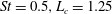 $\mathit{St}=0.5,L_{c}=1.25$
; (d)
$\mathit{St}=0.5,L_{c}=1.25$
; (d)
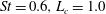 $\mathit{St}=0.6,L_{c}=1.0$
; (e)
$\mathit{St}=0.6,L_{c}=1.0$
; (e)
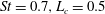 $\mathit{St}=0.7,L_{c}=0.5$
.
$\mathit{St}=0.7,L_{c}=0.5$
.

Figure 19. Comparison of the SPL obtained from LEE, experiments and propagation from a cylindrical surface at
 $R=1.3$
, with and without applying a Gaussian coherence envelope for the Mach 0.6 jet: (a)
$R=1.3$
, with and without applying a Gaussian coherence envelope for the Mach 0.6 jet: (a)
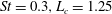 $\mathit{St}=0.3,L_{c}=1.25$
; (b)
$\mathit{St}=0.3,L_{c}=1.25$
; (b)
 $\mathit{St}=0.4,L_{c}=1.25$
; (c)
$\mathit{St}=0.4,L_{c}=1.25$
; (c)
 $\mathit{St}=0.5,L_{c}=1.0$
; (d)
$\mathit{St}=0.5,L_{c}=1.0$
; (d)
 $\mathit{St}=0.6,L_{c}=0.5$
; (e)
$\mathit{St}=0.6,L_{c}=0.5$
; (e)
 $\mathit{St}=0.7,L_{c}=0.25$
.
$\mathit{St}=0.7,L_{c}=0.25$
.
4.2. Coherence matching and far-field sound from a conical control surface
From figures 17–19, it can be seen that coherence matching along a cylindrical surface gives the right level of far-field sound but flattens the directivity. In particular, the directivity shape is not predicted accurately for low angles from the jet axis.
In order to determine whether this is caused by the cylindrical approximation of the measured surface, the coherence-matching process was adapted to a conical surface using the method developed by Reba et al. (Reference Reba, Narayanan and Colonius2010). In this case, the far-field PSD with coherence matching on the surface is computed as shown in (4.11). In this set-up,
 $\mathscr{R}$
and
$\mathscr{R}$
and
 ${\it\Theta}$
are defined in spherical polar coordinates with the origin placed at the projected apex upstream of the jet nozzle as shown in the schematic in figure 20:
${\it\Theta}$
are defined in spherical polar coordinates with the origin placed at the projected apex upstream of the jet nozzle as shown in the schematic in figure 20:
 $$\begin{eqnarray}\displaystyle \langle \hat{p}_{m}^{\prime }(\mathscr{R}^{\prime },{\it\Theta}^{\prime },{\it\omega})\hat{p}_{m}^{\ast \prime }(\mathscr{R}^{\prime },{\it\Theta}^{\prime },{\it\omega})\rangle & = & \displaystyle 4{\rm\pi}^{2}\sin ^{2}{\it\alpha}\iint P_{m}(\mathscr{R}_{1},\mathscr{R}_{2},{\it\omega})\frac{\partial g_{m}}{\partial {\it\Theta}}\left(\mathscr{R}_{1},{\it\alpha};\mathscr{R}^{\prime },{\it\Theta}^{\prime }\right)\nonumber\\ \displaystyle & & \displaystyle \times \,\frac{\partial g_{m}}{\partial {\it\Theta}}^{\ast }\left(\mathscr{R}_{2},{\it\alpha};\mathscr{R}^{\prime },{\it\Theta}^{\prime }\right)\,\text{d}r_{1}\,\text{d}r_{2}.\end{eqnarray}$$
Here,
 $g_{m}$
is a Green’s function tailored for the conical surface based on the reduced wave equation such that its value is set to zero on the surface;
$g_{m}$
is a Green’s function tailored for the conical surface based on the reduced wave equation such that its value is set to zero on the surface;
 $\mathscr{R}^{\prime }$
and
$\mathscr{R}^{\prime }$
and
 ${\it\Theta}^{\prime }$
indicate observer locations;
${\it\Theta}^{\prime }$
indicate observer locations;
 $P_{m}(\mathscr{R}_{1},\mathscr{R}_{2},{\it\omega})$
is the coherence-matched CSD of the near-field pressure on the conical surface, which is given by
$P_{m}(\mathscr{R}_{1},\mathscr{R}_{2},{\it\omega})$
is the coherence-matched CSD of the near-field pressure on the conical surface, which is given by
 $$\begin{eqnarray}P_{m}(\mathscr{R}_{1},\mathscr{R}_{2},{\it\omega})=\int \langle p_{m}^{\ast \prime }(\mathscr{R}_{1},{\it\alpha},t)p_{m}^{\prime }(\mathscr{R}_{2},{\it\alpha},t+{\it\tau})\rangle {\it\eta}(\mathscr{R}_{1},\mathscr{R}_{2},{\it\omega})\text{e}^{\text{i}{\it\omega}{\it\tau}}\,\text{d}{\it\tau}.\end{eqnarray}$$
 ${\it\eta}(\mathscr{R}_{1},\mathscr{R}_{2},{\it\omega})$
is the coherence profile along the line corresponding to the axisymmetric representation of the conical surface. It should be noted that prior to computing the near-field CSD, the pressure on the surface is windowed using a Butterworth filter to ensure that it decays smoothly to zero in the upstream parallel flow region, thereby preventing the occurrence of discontinuities. The results from propagating to the far field are shown in figure 21. It is evident that although this technique yields very similar results to the cylindrical surface approach, the mismatch in directivity persists and is more evident for low angles from the jet axis. This issue is further explored in § 6.
${\it\eta}(\mathscr{R}_{1},\mathscr{R}_{2},{\it\omega})$
is the coherence profile along the line corresponding to the axisymmetric representation of the conical surface. It should be noted that prior to computing the near-field CSD, the pressure on the surface is windowed using a Butterworth filter to ensure that it decays smoothly to zero in the upstream parallel flow region, thereby preventing the occurrence of discontinuities. The results from propagating to the far field are shown in figure 21. It is evident that although this technique yields very similar results to the cylindrical surface approach, the mismatch in directivity persists and is more evident for low angles from the jet axis. This issue is further explored in § 6.

Figure 20. Schematic showing the arrangement of the far-field propagation method using a conical surface.

Figure 21. Comparison of the SPL obtained for the Mach 0.6 turbulent jet from LEE, experiments and propagation from a conical surface that intersects the jet-nozzle plane at
 $R=0.8$
and has a cone half-angle of
$R=0.8$
and has a cone half-angle of
 ${\it\alpha}=8^{\circ }$
with and without applying coherence envelopes from experiments: (a)
${\it\alpha}=8^{\circ }$
with and without applying coherence envelopes from experiments: (a)
 $\mathit{St}=0.3$
, (b)
$\mathit{St}=0.3$
, (b)
 $\mathit{St}=0.4$
, (c)
$\mathit{St}=0.4$
, (c)
 $\mathit{St}=0.5$
, (d)
$\mathit{St}=0.5$
, (d)
 $\mathit{St}=0.6$
, (e)
$\mathit{St}=0.6$
, (e)
 $\mathit{St}=0.7$
.
$\mathit{St}=0.7$
.
5. The role of coherence decay on the near-field CSD
An investigation of the CSD on the cylindrical surface with and without coherence matching highlights the effect of a decaying coherence profile on the near field of a turbulent jet. From figure 22, it is evident that the coherence-matched CSD is more concentrated in space and hence more spread in the wavenumber domain when compared with the CSD obtained from the LEE results.

Figure 22. For the Mach 0.6, Strouhal 0.5 turbulent jet: (a) real part of the CSD without coherence matching, (b) real part of the CSD with coherence matching, (c) Fourier transform in space of the CSD without coherence matching, (d) Fourier transform in space of the CSD with coherence matching. The lines in grey denote the wavenumbers corresponding to sonic phase speeds defined by
 $k_{\infty }={\it\omega}/c_{\infty }$
.
$k_{\infty }={\it\omega}/c_{\infty }$
.
The grey lines drawn in figure 22 represent wavenumbers corresponding to sonic phase speeds, and only wavenumbers lying within the square bounded by these lines correspond to acoustic radiation (Cavalieri & Agarwal Reference Cavalieri and Agarwal2014). The impact of coherence matching on sound radiation can be understood by noting that most of the source energy for the original CSD without coherence matching lies outside this square area in the wavenumber domain (figure 22 c). This is not the case for the coherence-matched CSD (figure 22 d), where the supersonic tail is spread more into this region due to its narrow shape in the spatial domain, as shown by figure 22(b). The SPLs for the coherence-matched cases are hence higher in magnitude since only the supersonic tail inside the square area is related to far-field sound, and this is much larger in figure 22(d) than in figure 22(c).
The effect of decaying coherence is, therefore, to spread the hydrodynamic component of the source on to acoustic wavenumbers, resulting in a more efficient acoustic source. This result demonstrates the main reason behind the failure of linear models in matching the far-field SPL for subsonic turbulent jets. Because of the radial decay of the hydrodynamic component of the pressure field, the far-field SPL computed depends on both the coherence profile and the location of the surface at which the CSD is measured. Figure 23 demonstrates results from the parametric study conducted for figures 18 and 19 using Gaussian coherence envelopes for the Mach 0.6, Strouhal number 0.5 case. The far-field SPL computed using Gaussian envelopes of varying coherence length scales,
 $L_{c}$
(from 0.5 to 2.5 in increments of 0.5), is shown for cylindrical surfaces at
$L_{c}$
(from 0.5 to 2.5 in increments of 0.5), is shown for cylindrical surfaces at
 $R=1.3$
and
$R=1.3$
and
 $R=0.6$
. The results show that the far-field SPL computed is very sensitive to the coherence profile, in particular to the coherence length scale,
$R=0.6$
. The results show that the far-field SPL computed is very sensitive to the coherence profile, in particular to the coherence length scale,
 $L_{c}$
. A minor change in
$L_{c}$
. A minor change in
 $L_{c}$
has a large effect on the far-field pressure (note that SPL is computed in
$L_{c}$
has a large effect on the far-field pressure (note that SPL is computed in
 $\text{dB}$
). Since the coherence length scale varies as the length scale of the wavepacket, this observation can guide future development of models that do not depend on experimentally obtained coherence functions. In general, the directivity is flatter for smaller length scales and surfaces further away from the jet axis. A larger length scale is needed to match the peak SPL for
$\text{dB}$
). Since the coherence length scale varies as the length scale of the wavepacket, this observation can guide future development of models that do not depend on experimentally obtained coherence functions. In general, the directivity is flatter for smaller length scales and surfaces further away from the jet axis. A larger length scale is needed to match the peak SPL for
 $R=0.6$
than for
$R=0.6$
than for
 $R=1.3$
. The issue of surface location is discussed in more detail in § 6.
$R=1.3$
. The issue of surface location is discussed in more detail in § 6.

Figure 23. For the Mach 0.6, Strouhal 0.5 turbulent jet, far-field SPL computed using a Gaussian coherence profile with various coherence length scales,
 $L_{c}$
, from 0.5 (darkest grey) to 2.5 (lightest grey) in increments of 0.5, propagating from a cylindrical enclosing surface at (a)
$L_{c}$
, from 0.5 (darkest grey) to 2.5 (lightest grey) in increments of 0.5, propagating from a cylindrical enclosing surface at (a)
 $R=1.3$
and (b)
$R=1.3$
and (b)
 $R=0.6$
.
$R=0.6$
.
6. Surface location and far-field directivity
Since the coherence profiles used for the Mach 0.6 jet are obtained directly from experiments, the inaccuracy in predicting low-angle directivity by the coherence-matching process is probably due to one or both of two possible reasons – inaccuracies in the coherence measurements or inadequate hydrodynamic signature at the enclosing control surface. While the first reason is beyond the scope of this work and is best addressed by more detailed experimental research in the future, the second can be investigated by examining the surface CSD on moving the propagation surface closer to the jet axis where the hydrodynamics is known to be a stronger component. This corresponds to using a cylinder of a smaller radius,
 $R$
, for the cylindrical propagation method and a smaller half-angle,
$R$
, for the cylindrical propagation method and a smaller half-angle,
 ${\it\alpha}$
, or a smaller intercept with the jet-nozzle plane for the conical propagation method.
${\it\alpha}$
, or a smaller intercept with the jet-nozzle plane for the conical propagation method.
Since coherence measurements are unavailable for these locations, the model Gaussian coherence profile from (4.4) is used to investigate the effect of surface location in relation to coherence matching.
Figure 24 shows the effect of moving the cylindrical surface closer to the jet axis (
 $R=0.6$
) on the sound propagated to the far field. A parametric analysis of coherence length scales was carried out in the same manner at this location as in § 4.1 but with a finer resolution,
$R=0.6$
) on the sound propagated to the far field. A parametric analysis of coherence length scales was carried out in the same manner at this location as in § 4.1 but with a finer resolution,
 ${\rm\Delta}L_{c}=0.1$
. It was observed first that a larger coherence length scale is required in general for cylindrical surfaces closer to the jet-nozzle lip line to obtain a far-field SPL match. Most importantly however, the directivity shape for low angles is matched better if the surface is moved closer to the jet axis, although the discrepancy now increases for larger angles. As mentioned in earlier sections, it is important to have the surface outside the source region where the flow is irrotational as the propagation techniques used are based on the linear wave equation.
${\rm\Delta}L_{c}=0.1$
. It was observed first that a larger coherence length scale is required in general for cylindrical surfaces closer to the jet-nozzle lip line to obtain a far-field SPL match. Most importantly however, the directivity shape for low angles is matched better if the surface is moved closer to the jet axis, although the discrepancy now increases for larger angles. As mentioned in earlier sections, it is important to have the surface outside the source region where the flow is irrotational as the propagation techniques used are based on the linear wave equation.

Figure 24. Comparison of the SPL obtained using propagation from a cylindrical surface for the Mach 0.6, Strouhal 0.5 turbulent jet with and without using a Gaussian coherence profile of coherence length scale
 $L_{c}$
at (a)
$L_{c}$
at (a)
 $R=1.3$
with
$R=1.3$
with
 $L_{c}=1.0$
and (b)
$L_{c}=1.0$
and (b)
 $R=0.6$
with
$R=0.6$
with
 $L_{c}=1.9$
.
$L_{c}=1.9$
.
A more quantitative analysis of the effect of surface location is impossible without accurate coherence measurements at these locations. We can, however, compare the CSDs on both cylindrical surfaces at
 $R=1.3$
and
$R=1.3$
and
 $R=0.6$
to understand the difference in directivity shapes. Figure 25 shows the CSDs at these two locations with and without coherence matching.
$R=0.6$
to understand the difference in directivity shapes. Figure 25 shows the CSDs at these two locations with and without coherence matching.

Figure 25. For the Mach 0.6, Strouhal 0.5 turbulent jet: Fourier transform in space of the CSD on a cylindrical surface at (a)
 $R=1.3$
without coherence matching, (b)
$R=1.3$
without coherence matching, (b)
 $R=0.6$
without coherence matching, (c)
$R=0.6$
without coherence matching, (c)
 $R=1.3$
with coherence matching using a Gaussian coherence profile with
$R=1.3$
with coherence matching using a Gaussian coherence profile with
 $L_{c}=1.0$
and (d)
$L_{c}=1.0$
and (d)
 $R=0.6$
with coherence matching using a Gaussian coherence profile with
$R=0.6$
with coherence matching using a Gaussian coherence profile with
 $L_{c}=1.9$
. The lines in grey denote the wavenumbers corresponding to sonic phase speeds defined by
$L_{c}=1.9$
. The lines in grey denote the wavenumbers corresponding to sonic phase speeds defined by
 $k_{\infty }={\it\omega}/c_{\infty }$
. The maximum contour colour has been lowered to
$k_{\infty }={\it\omega}/c_{\infty }$
. The maximum contour colour has been lowered to
 $1\times 10^{4}$
to better highlight the components inside the square bounded by these lines.
$1\times 10^{4}$
to better highlight the components inside the square bounded by these lines.
As expected, the source energy outside the square region bounded by wavenumbers corresponding to sonic phase speeds is larger and more distributed in figure 25(b) than 25(a), since this corresponds to the hydrodynamic component that is more prominent closer to the jet axis. The use of a Gaussian coherence profile that results in a match in the far-field SPL causes this hydrodynamic component to spread into the square region in both cases, as shown in 25(c,d). However, inside the square region, there is a sharper decrease to zero for the
 $R=0.6,L_{c}=1.9$
case than for the
$R=0.6,L_{c}=1.9$
case than for the
 $R=1.3,L_{c}=1.0$
case. This is seen more clearly in figure 26, which compares the profiles of the coherence-matched CSD along the diagonal.
$R=1.3,L_{c}=1.0$
case. This is seen more clearly in figure 26, which compares the profiles of the coherence-matched CSD along the diagonal.

Figure 26. For the Mach 0.6, Strouhal 0.5 turbulent jet: Fourier transform in space of the coherence-matched CSD on a cylindrical surface along the diagonal (
 $k_{z_{1}}=-k_{z_{2}}$
) at
$k_{z_{1}}=-k_{z_{2}}$
) at
 $R=1.3$
with
$R=1.3$
with
 $L_{c}=1.0$
and at
$L_{c}=1.0$
and at
 $R=0.6$
with
$R=0.6$
with
 $L_{c}=1.9$
. The vertical lines in black denote the wavenumbers corresponding to sonic phase speeds defined by
$L_{c}=1.9$
. The vertical lines in black denote the wavenumbers corresponding to sonic phase speeds defined by
 $k_{\infty }={\it\omega}/c_{\infty }$
.
$k_{\infty }={\it\omega}/c_{\infty }$
.
The far-field SPL is a function of the CSD only for the range of wavenumbers within the square area bounded by the wavenumbers corresponding to sonic phase speeds. This was shown in Cavalieri & Agarwal (Reference Cavalieri and Agarwal2014) using the Green’s function for the Helmholtz equation on the line source described in (4.2). By noting that the approximate far-field solution is in the form of a double Fourier transform, they showed that the far-field PSD at a location
 $\boldsymbol{x}$
is given by
$\boldsymbol{x}$
is given by
 $$\begin{eqnarray}\langle p^{\prime }(\boldsymbol{x},{\it\omega})p^{\ast \prime }(\boldsymbol{x},{\it\omega})\rangle \approx \frac{1}{8{\rm\pi}x^{2}}\mathscr{S}\left(k_{z_{1}}=-k_{\infty }\cos {\it\theta},k_{z_{2}}=k_{\infty }\cos {\it\theta}\right),\end{eqnarray}$$
where
 $x$
is the distance between the origin (taken to be the centre of the jet nozzle) and the observer,
$x$
is the distance between the origin (taken to be the centre of the jet nozzle) and the observer,
 ${\it\theta}$
is the polar angle between the source and the jet axis and
${\it\theta}$
is the polar angle between the source and the jet axis and
 $k_{\infty }={\it\omega}/c_{\infty }$
is the wavenumber corresponding to sonic phase speeds;
$k_{\infty }={\it\omega}/c_{\infty }$
is the wavenumber corresponding to sonic phase speeds;
 $\mathscr{S}$
is the double Fourier transform of the CSD of the line source. Therefore, the distribution of source energy in the region
$\mathscr{S}$
is the double Fourier transform of the CSD of the line source. Therefore, the distribution of source energy in the region
 $|k_{z_{1}}|\leqslant k_{\infty }$
and
$|k_{z_{1}}|\leqslant k_{\infty }$
and
 $|k_{z_{2}}|\leqslant k_{\infty }$
determines the far-field directivity shape. The more distributed profile which corresponds to
$|k_{z_{2}}|\leqslant k_{\infty }$
determines the far-field directivity shape. The more distributed profile which corresponds to
 $R=1.3$
,
$R=1.3$
,
 $L_{c}=1.0$
thus results in a flatter directivity shape, whereas the less distributed profile of
$L_{c}=1.0$
thus results in a flatter directivity shape, whereas the less distributed profile of
 $R=0.6$
,
$R=0.6$
,
 $L_{c}=1.9$
results in a sharper, more superdirective shape, similar to what is observed in the experimental results.
$L_{c}=1.9$
results in a sharper, more superdirective shape, similar to what is observed in the experimental results.
Similar conclusions were drawn from carrying out a similar analysis of the conical surface propagation method as shown in figures 27, 28 and 29. Here, the intersection of the conical surface with the jet-nozzle plane was lowered to
 $R=0.6$
and the cone half-angle was also reduced to
$R=0.6$
and the cone half-angle was also reduced to
 ${\it\alpha}=4^{\circ }$
to bring the surface closer to the flow region.
${\it\alpha}=4^{\circ }$
to bring the surface closer to the flow region.

Figure 27. Comparison of the SPL obtained using propagation from a conical surface for the Mach 0.6, Strouhal 0.5 turbulent jet with and without using a Gaussian coherence profile of coherence length scale
 $L_{c}$
at (a)
$L_{c}$
at (a)
 $R=0.8$
,
$R=0.8$
,
 ${\it\alpha}=8^{\circ }$
with
${\it\alpha}=8^{\circ }$
with
 $L_{c}=1.0$
and (b)
$L_{c}=1.0$
and (b)
 $R=0.6$
,
$R=0.6$
,
 ${\it\alpha}=4^{\circ }$
with
${\it\alpha}=4^{\circ }$
with
 $L_{c}=1.5$
.
$L_{c}=1.5$
.

Figure 28. For the Mach 0.6, Strouhal 0.5 turbulent jet: Fourier transform in space of the CSD on a conical surface at (a)
 $R=0.8,{\it\alpha}=8^{\circ }$
without coherence matching, (b)
$R=0.8,{\it\alpha}=8^{\circ }$
without coherence matching, (b)
 $R=0.6,{\it\alpha}=4^{\circ }$
without coherence matching, (c)
$R=0.6,{\it\alpha}=4^{\circ }$
without coherence matching, (c)
 $R=0.8,{\it\alpha}=8^{\circ }$
with coherence matching using a Gaussian coherence profile with
$R=0.8,{\it\alpha}=8^{\circ }$
with coherence matching using a Gaussian coherence profile with
 $L_{c}=1.0$
and (d)
$L_{c}=1.0$
and (d)
 $R=0.6,{\it\alpha}=4^{\circ }$
with coherence matching using a Gaussian coherence profile with
$R=0.6,{\it\alpha}=4^{\circ }$
with coherence matching using a Gaussian coherence profile with
 $L_{c}=1.5$
. The lines in grey denote the wavenumbers corresponding to sonic phase speeds defined by
$L_{c}=1.5$
. The lines in grey denote the wavenumbers corresponding to sonic phase speeds defined by
 $k_{\infty }={\it\omega}/c_{\infty }$
. The maximum contour colour has been lowered to
$k_{\infty }={\it\omega}/c_{\infty }$
. The maximum contour colour has been lowered to
 $1\times 10^{4}$
to better highlight the components inside the square bounded by these lines.
$1\times 10^{4}$
to better highlight the components inside the square bounded by these lines.

Figure 29. For the Mach 0.6, Strouhal 0.5 turbulent jet: Fourier transform in space of the coherence-matched CSD on a conical surface along the diagonal (
 $k_{\mathscr{R}_{1}}=-k_{\mathscr{R}_{2}}$
) at
$k_{\mathscr{R}_{1}}=-k_{\mathscr{R}_{2}}$
) at
 $R=0.8,{\it\alpha}=8^{\circ }$
with
$R=0.8,{\it\alpha}=8^{\circ }$
with
 $L_{c}=1.0$
and at
$L_{c}=1.0$
and at
 $R=0.6,{\it\alpha}=4^{\circ }$
with
$R=0.6,{\it\alpha}=4^{\circ }$
with
 $L_{c}=1.5$
. The vertical lines in black denote the wavenumbers corresponding to sonic phase speeds defined by
$L_{c}=1.5$
. The vertical lines in black denote the wavenumbers corresponding to sonic phase speeds defined by
 $k_{\infty }={\it\omega}/c_{\infty }$
.
$k_{\infty }={\it\omega}/c_{\infty }$
.
7. Conclusions and future work
The conclusions of the study were twofold; the first provides an understanding of the near-field dynamics and the second suggests an explanation of the far-field sound generated. First, it was found that for axisymmetric modes, the LEE simulations show that the near field appears to consist largely of linear wavepackets, consistent with previous works. A model of the near-field dynamics was developed using the LEE, and it was seen that as with existing models using LPSE, this agrees with the experimental results up to the end of the potential core. Downstream of this region, the LEE results deviate from experimental results but errors are reduced when compared with LPSE. This improvement can be attributed to the less restrictive hypothesis in the derivation of the model. For instance, the jet is not considered as a slowly diverging flow, and a wavepacket shape is not assumed a priori.
However, these linear wavepackets were found to produce very little sound compared with the sound field obtained from experiments, with a mismatch of more than an order of magnitude compared with the experimental results. The LEE, therefore, did not yield good predictions of far-field sound despite close statistical agreement for the near field. In order to explain this discrepancy, the proposition by Cavalieri & Agarwal (Reference Cavalieri and Agarwal2014) that coherence matching is a necessary condition for a match in far-field radiation, in addition to an agreement of other statistical properties, was tested. This was done by constructing a boundary value formulation in which the two-point CSD at a near-field surface was matched with experimental values and then the linear wave equation was solved by an integral method to propagate the solution to the far field. The resulting far-field SPLs show improved agreement with the experimental measurements of far-field SPLs. Furthermore, the use of Gaussian coherence envelopes with specified length scales was also shown to give reasonable agreement with experimental SPLs. A model was thus developed in which all aspects are linear except the coherence profile and the time-invariant mean flow where all of the nonlinearity is assumed to be confined.
Although the SPL results come closer to the experimental results with coherence matching, it was observed that especially for low angles from the jet axis, the directivity shape for far-field sound from the coherence-matched near field is flatter and therefore inconsistent with the superdirective nature of the experimental measurements. It was found, by varying the location of the surface on which coherence was matched, that the use of surfaces closer to the flow region allows for a better match of low-angle directivity. This is because coherence matching primarily modifies the hydrodynamic component of the two-point CSD on the surface, and so it is important for the surfaces to be as close as possible to the flow region while ensuring that the linear wave equation effectively describes the dynamics at the surface. It should be noted, however, that this analysis was conducted using the model Gaussian coherence profiles, as corresponding experimental measurements at these locations, resolved into azimuthal wavenumbers, are unavailable in the existing literature.
The model developed here is not meant to be predictive but serves to demonstrate that coherence decay is the main missing feature of linear models of turbulent subsonic jets pertaining to sound radiation. Therefore, the results of the present work indicate that future work in this direction should be focused on more accurate and extensive experimental measurements of the near-field coherence. These may be compared with the coherence length scales predicted by the Gaussian envelope models developed here. It may also be desirable to investigate different control surfaces that better capture the hydrodynamics of the turbulent jet.
Apart from the mean flow profiles that are readily available for jets, the only empirical component in our model is in the description of coherence profiles. It was shown, using Gaussian model envelopes, that the far-field solution is particularly sensitive to the coherence length scale, a finding that may prove useful for predictive models developed in the future that do not depend on measured coherence profiles. This underscores the importance of determining the flow features related to the decaying coherence profiles for a more complete understanding of jet noise in subsonic turbulent jets. Some work in this direction has been done by Cavalieri & Agarwal (Reference Cavalieri and Agarwal2014) and Zhang et al. (Reference Zhang, Jordan, Lehnasch, Cavalieri and Agarwal2014), who have related coherence decay with nonlinearity. In order to obtain predictions of the radiated sound by subsonic jets, reduced-order linear wavepacket models such as LPSE or LEE should be extended in order to account for coherence decay in some way. Although this work does not address the question of which flow features underpin coherence decay, we have shown that a match of the coherence profiles is the main missing feature of linear wavepacket models in order to predict the radiated sound.
Appendix A. Azimuthal decomposition of CSD and coherence
Michalke & Fuchs (Reference Michalke and Fuchs1975) showed that for round jets, the two-point CSD for any azimuthal mode depends only on the constituent of the pressure field for that azimuthal mode. As shown below, a similar argument can be made for the coherence between two points.
Consider a near pressure field
 $p^{\prime }(z,r,{\it\phi},t)$
, which can be expanded as a Fourier series in the azimuthal angle,
$p^{\prime }(z,r,{\it\phi},t)$
, which can be expanded as a Fourier series in the azimuthal angle,
 ${\it\phi}$
, as
${\it\phi}$
, as
 $$\begin{eqnarray}p^{\prime }(z,r,{\it\phi},t)=\mathop{\sum }_{m=-\infty }^{\infty }p_{m}^{\prime }(z,r,t)\text{e}^{-\text{i}m{\it\phi}},\end{eqnarray}$$
where
 $$\begin{eqnarray}p_{m}^{\prime }(z,r,t)=\frac{1}{2{\rm\pi}}\int _{0}^{2{\rm\pi}}p^{\prime }(z,r,{\it\phi},t)\text{e}^{\text{i}m{\it\phi}}\,\text{d}{\it\phi}.\end{eqnarray}$$
The CSD between two points can be written as
 $$\begin{eqnarray}\displaystyle & & \displaystyle P(z_{1},r_{1},{\it\phi}_{1},z_{2},r_{2},{\it\phi}_{2},{\it\omega})\nonumber\\ \displaystyle & & \displaystyle \quad =\int _{-\infty }^{\infty }\frac{1}{T}\int _{t}^{t+T}p^{\prime }(z_{1},r_{1},{\it\phi}_{1},t_{1})p^{\ast \prime }(z_{2},r_{2},{\it\phi}_{2},t_{1}+{\it\tau})\text{e}^{\text{i}{\it\omega}{\it\tau}}\,\text{d}t_{1}\,\text{d}{\it\tau}\nonumber\\ \displaystyle & & \displaystyle \quad =\mathop{\sum }_{m=-\infty }^{\infty }\mathop{\sum }_{n=-\infty }^{\infty }\int _{-\infty }^{\infty }\frac{1}{T}\int _{t}^{t+T}p_{m}^{\prime }(z_{1},r_{1},t_{1})p_{n}^{\ast \prime }(z_{2},r_{2},t_{1}+{\it\tau})\text{e}^{-\text{i}m{\it\phi}_{1}}\text{e}^{\text{i}n{\it\phi}_{2}}\text{e}^{\text{i}{\it\omega}{\it\tau}}\,\text{d}t_{1}\,\text{d}{\it\tau}.\qquad\end{eqnarray}$$
Because of the symmetry conditions in a circular jet (circumferential homogeneity), the CSD can only depend on
 ${\rm\Delta}{\it\phi}={\it\phi}_{1}-{\it\phi}_{2}$
and not on
${\rm\Delta}{\it\phi}={\it\phi}_{1}-{\it\phi}_{2}$
and not on
 ${\it\phi}_{1}$
and
${\it\phi}_{1}$
and
 ${\it\phi}_{2}$
separately. That is,
${\it\phi}_{2}$
separately. That is,
 $$\begin{eqnarray}P(z_{1},r_{1},{\it\phi}_{1},z_{2},r_{2},{\it\phi}_{2},{\it\omega})=P(z_{1},r_{1},z_{2},r_{2},{\rm\Delta}{\it\phi},{\it\omega}).\end{eqnarray}$$
Additionally,
 $P(z_{1},r_{1},z_{2},r_{2},{\rm\Delta}{\it\phi},{\it\omega})$
must be a periodic function with respect to
$P(z_{1},r_{1},z_{2},r_{2},{\rm\Delta}{\it\phi},{\it\omega})$
must be a periodic function with respect to
 ${\rm\Delta}{\it\phi}$
. Therefore, the CSD can be expanded as a Fourier series in
${\rm\Delta}{\it\phi}$
. Therefore, the CSD can be expanded as a Fourier series in
 $({\it\phi}_{1}-{\it\phi}_{2})$
:
$({\it\phi}_{1}-{\it\phi}_{2})$
:
 $$\begin{eqnarray}P(z_{1},r_{1},{\it\phi}_{1},z_{2},r_{2},{\it\phi}_{2},{\it\omega})=\mathop{\sum }_{m^{\prime }=-\infty }^{\infty }P_{m^{\prime }}(z_{1},r_{1},z_{2},r_{2},{\it\omega})\text{e}^{-\text{i}m^{\prime }({\it\phi}_{1}-{\it\phi}_{2})},\end{eqnarray}$$
where the complex-valued Fourier coefficients
 $P_{m^{\prime }}$
are defined as
$P_{m^{\prime }}$
are defined as
 $$\begin{eqnarray}P_{m^{\prime }}(z_{1},r_{1},z_{2},r_{2},{\it\omega})=\frac{1}{(2{\rm\pi})^{2}}\int _{0}^{2{\rm\pi}}\int _{0}^{2{\rm\pi}}P(z_{1},r_{1},{\it\phi}_{1},z_{2},r_{2},{\it\phi}_{2},{\it\omega})\text{e}^{\text{i}m^{\prime }({\it\phi}_{1}-{\it\phi}_{2})}\,\text{d}{\it\phi}_{1}\,\text{d}{\it\phi}_{2}.\end{eqnarray}$$
Therefore,
 $$\begin{eqnarray}P_{m^{\prime }}(z_{1},r_{1},z_{2},r_{2},{\it\omega})=\frac{1}{(2{\rm\pi})^{2}}\int _{0}^{2{\rm\pi}}\int _{0}^{2{\rm\pi}}\mathop{\sum }_{m=-\infty }^{\infty }\mathop{\sum }_{n=-\infty }^{\infty }\int _{-\infty }^{\infty }\frac{1}{T}\int _{t}^{t+T}I_{1}\,\text{d}t_{1}\,\text{d}{\it\tau}\,\text{d}{\it\phi}_{1}\,\text{d}{\it\phi}_{2},\end{eqnarray}$$
where
 $$\begin{eqnarray}I_{1}=p_{m}^{\prime }(z_{1},r_{1},t_{1})p_{n}^{\ast \prime }(z_{2},r_{2},t_{1}+{\it\tau})\text{e}^{-\text{i}m{\it\phi}_{1}}\text{e}^{\text{i}n{\it\phi}_{2}}\text{e}^{\text{i}m^{\prime }({\it\phi}_{1}-{\it\phi}_{2})}\text{e}^{\text{i}{\it\omega}{\it\tau}}.\end{eqnarray}$$
Since the
 ${\it\phi}_{1}$
and
${\it\phi}_{1}$
and
 ${\it\phi}_{2}$
integrals are non-zero only for
${\it\phi}_{2}$
integrals are non-zero only for
 $m=m^{\prime }$
and
$m=m^{\prime }$
and
 $n=m^{\prime }$
respectively, we have
$n=m^{\prime }$
respectively, we have
 $$\begin{eqnarray}P_{m^{\prime }}(z_{1},r_{1},z_{2},r_{2},{\it\omega})=\frac{1}{(2{\rm\pi})^{2}}\int _{0}^{2{\rm\pi}}\int _{0}^{2{\rm\pi}}\int _{-\infty }^{\infty }\frac{1}{T}\int _{t}^{t+T}I_{2}\,\text{d}t_{1}\,\text{d}{\it\tau}\,\text{d}{\it\phi}_{1}\,\text{d}{\it\phi}_{2},\end{eqnarray}$$
where
 $$\begin{eqnarray}I_{2}=p_{m^{\prime }}^{\prime }(z_{1},r_{1},t_{1})p_{m^{\prime }}^{\ast \prime }(z_{2},r_{2},t_{1}+{\it\tau})\text{e}^{-\text{i}m^{\prime }{\it\phi}_{1}}\text{e}^{\text{i}m^{\prime }{\it\phi}_{2}}\text{e}^{\text{i}m^{\prime }({\it\phi}_{1}-{\it\phi}_{2})}\text{e}^{\text{i}{\it\omega}{\it\tau}}.\end{eqnarray}$$
Thus, we arrive at
 $$\begin{eqnarray}\displaystyle P_{m^{\prime }}(z_{1},r_{1},z_{2},r_{2},{\it\omega}) & = & \displaystyle \int _{-\infty }^{\infty }\frac{1}{T}\int _{t}^{t+T}p_{m^{\prime }}^{\prime }(z_{1},r_{1},t_{1})p_{m^{\prime }}^{\ast \prime }(z_{2},r_{2},t_{1}+{\it\tau})\text{e}^{\text{i}{\it\omega}{\it\tau}}\,\text{d}t_{1}\,\text{d}{\it\tau}\nonumber\\ \displaystyle & = & \displaystyle \int _{-\infty }^{\infty }\left\langle p_{m^{\prime }}^{\prime }(z_{1},r_{1},t_{1})p_{m^{\prime }}^{\ast \prime }(z_{2},r_{2},t_{1}+{\it\tau})\right\rangle \text{e}^{\text{i}{\it\omega}{\it\tau}}\,\text{d}{\it\tau}.\end{eqnarray}$$
Hence, each
 $P_{m^{\prime }}$
is determined solely by the corresponding
$P_{m^{\prime }}$
is determined solely by the corresponding
 $m^{\prime }$
th azimuthal constituent of the pressure itself. Consequently, the CSD for the axisymmetric mode
$m^{\prime }$
th azimuthal constituent of the pressure itself. Consequently, the CSD for the axisymmetric mode
 $m^{\prime }=0$
depends on the axisymmetric constituent of the pressure field. That is,
$m^{\prime }=0$
depends on the axisymmetric constituent of the pressure field. That is,
 $$\begin{eqnarray}P_{0}(z_{1},r_{1},z_{2},r_{2},{\it\omega})=\int _{-\infty }^{\infty }\left\langle p_{0}^{\prime }(z_{1},r_{1},t_{1})p_{0}^{\ast \prime }(z_{2},r_{2},t_{1}+{\it\tau})\right\rangle \text{e}^{\text{i}{\it\omega}{\it\tau}}\,\text{d}{\it\tau}.\end{eqnarray}$$
The coherence between two points for the axisymmetric case is thus defined using the CSD for
 $m^{\prime }=0$
as
$m^{\prime }=0$
as
 $$\begin{eqnarray}{\it\eta}^{2}(z_{1},r_{1},z_{2},r_{2},{\it\omega})=\frac{|\langle p_{0}^{\prime }(z_{1},r_{1},{\it\omega})p_{0}^{\ast \prime }(z_{2},r_{2},{\it\omega})\rangle |^{2}}{\langle |p_{0}^{\prime }(z_{1},r_{1},{\it\omega})|^{2}\rangle \langle |p_{0}^{\prime }(z_{2},r_{2},{\it\omega})|^{2}\rangle }.\end{eqnarray}$$
Appendix B. Schematic of boundary value formulations
Figure 30 shows the schematic of the two enclosing surfaces used to formulate boundary value formulations in the present work. These diagrams are meant to be illustrative only and are therefore not to scale.

Figure 30. Schematic of boundary value formulations (not to scale) for the cylindrical enclosing surface and conical enclosing surface.


