INTRODUCTION
Calibration is of fundamental importance to the radiocarbon (14C) method. It is only through calibration that changing levels of atmospheric 14C can be accounted for, and an estimate of the true age of a sample in calendar years established. The development of the international calibration curves (Hogg et al. Reference Hogg, Hua, Blackwell, Niu, Buck, Guilderson, Heaton, Palmer, Reimer and Reimer2013; Reimer et al. Reference Reimer, Bard, Bayliss, Beck, Blackwell, Bronk Ramsey, Buck, Cheng, Edwards and Friedrich2013) has enabled researchers to compare their dates to a well-established and robust set of standard measurements.
The curves from 0 to 13,900 cal BP have mostly been constructed using 14C measurements on decadal sections of tree-ring growth, which smooth out any variations in 14C shorter than 10 years. Although the existence of variability on a shorter time scale than this has been recognized previously (e.g. Damon et al. Reference Damon, Lerman and Long1978), the construction of a calibration curve at a higher resolution has been impractical. Additionally, while noting that major peaks and troughs do exist, Bronk Ramsey et al. (Reference Bronk Ramsey, Buck, Manning, Reimer and van der Plicht2006) observed that much short-term variability is noise that cancels itself out after only a few years, especially within the uncertainty associated with typical 14C measurements. More recently, however, the significance of substantial short-term fluctuations in 14C has been emphasized (Miyake et al. Reference Miyake, Nagaya, Masuda and Nakamura2012, Reference Miyake, Masuda and Nakamura2013; Güttler et al. Reference Güttler, Adolphi, Beer, Bleicher, Boswijk, Christl, Hogg, Palmer, Vockenhuber and Wacker2015), while limitations with decadally averaged curves have been highlighted (Bayliss et al. Reference Bayliss, Marshall, Tyers, Bronk Ramsey, Cook, Freeman and Griffiths2017). What is more, Wacker et al. (Reference Wacker, Güttler, Hurni, Synal and Walti2014) demonstrated how these short-lived fluctuations can be used to obtain highly precise dates on individual samples.
These observations demonstrate the need for a re-examination of the potential of a single-year calibration curve. The construction of such a curve would depend on tree-ring seasonality and the processes that govern the incorporation of 14C into individual rings. This can be focused onto two key issues: variations in atmospheric 14C, the reservoir from which trees take up carbon; and the physiological mechanism by which it is deposited into rings during growth. To investigate seasonality in these two factors we obtained dates on earlywood and latewood fractions of known-age annual tree rings from England dated between AD 1352 and AD 1442. This time period was selected in response to work by Bayliss et al. (Reference Bayliss, Marshall, Tyers, Bronk Ramsey, Cook, Freeman and Griffiths2017) who observed unexplained incorrect wiggle-matches on known-age tree-ring sequences dating to this time. It was hypothesized that seasonal variations in the atmospheric 14C reservoir would be approximately proportional to the rate of 14C production while physiological factors would be less predictable. In this way, it was hoped that the presence of a seasonal signal in tree ring 14C could be identified.
Plant Physiology
The utility of wood for examining the 14C method depends on the relationship between the 14C content in a growth ring, and atmospheric 14C during the year in which the ring was formed. Specifically, it is assumed that the 14C content in a ring represents atmospheric levels during that particular growing period. This assumption, however, could be undermined by the storage and later remobilization of photosynthates by trees. Keel et al. (Reference Keel, Siegwolf and Kötner2006) demonstrated that trees preferentially use recent photosynthates for growth, yet it has long been recognized that plants do not immediately convert all photosynthesized carbon into structural tissues. The chemistry and metabolic processes that govern this nonstructural carbon (NSC) are incompletely understood, and are only now becoming an intensively investigated topic (Dietze et al. Reference Dietze, Sala, Carbone, Czimczik, Mantooth, Richardson and Vargas2014; Gessler and Treydte Reference Gessler and Treydte2016). Storage in plants has been conceptualized in a number of different ways and is recognized as occurring across a range of different time scales from within a single day to across multiple years (Chapin et al. Reference Chapin, Schulze and Mooney1990; Dietze et al. Reference Dietze, Sala, Carbone, Czimczik, Mantooth, Richardson and Vargas2014). The most obvious case of storage occurring at the seasonal scale, however, is in deciduous trees that use NSC to produce leaves, while some ring-porous species such as oak even begin radial growth before their leaves have been produced by using stored carbohydrates (Speer Reference Speer2010: 46–47).
This initial use of NSCs to “kick start” growth at the beginning of the growing season has been well established by the monitoring of sugar levels in tree trunks throughout the year (Sauter Reference Sauter1980; Höll Reference Höll1985; Barbaroux and Bréda Reference Barbaroux and Bréda2002). Of greatest relevance to this paper, however, is the age of the remobilized carbon. Gaudinski et al. (Reference Gaudinski, Torn, Riley, Swanston, Trumbore, Joslin, Majdi, Dawson and Hanson2009) used 14C dates to argue that in two oak species and red maple the carbon used for leaf growth is no more than one year old, suggesting that the carbon deposited in earlywood is of a similar age. In contrast, Muhr et al. (Reference Muhr, Messier, Delagrange, Trumbore, Xu and Hartmann2016) used both 14C and 13C to argue that the sugars deposited in the sap of maple xylem derived from a mixed pool of carbon that was turned over every 3–5 years. What is becoming increasingly clear, is that the distinction between pools with different turnover times is of the utmost importance (Dietze et al. Reference Dietze, Sala, Carbone, Czimczik, Mantooth, Richardson and Vargas2014; Richardson et al. Reference Richardson, Carbone, Huggett, Furze, Czimczik, Walker, Xu, Schaberg and Murakami2015). Such differences are averaged out when dates are taken on multiple years of growth, but when tree rings are measured at a higher resolution there is potential for this to influence results.
In addition to this regular use of stored carbon, recent studies have demonstrated that trees can remobilize carbon after more than a decade. This is most often connected to major disturbance events, and experiments with defoliating young trees have shown that those with a larger store of NSC were more likely to survive. NSC remobilized after this length of time is more likely to go to roots or shoots than annual growth rings, and it is generally in these structures where it is found. For example, Carbone et al. (Reference Carbone, Czimczik, Keenan, Murakami, Pederson, Schaberg, Xu and Richardson2013) showed that shoots sprouting from a red maple trunk were formed from NSC that was up to 17 years old, while Richardson et al. (Reference Richardson, Carbone, Keenan, Czimczik, Hollinger, Murakami, Schaberg and Xu2013) showed that starches in the trunk of red maple were between 7 and 14 years old. Whether such old carbon is incorporated into structural compounds in tree trunks has not yet been established, but the potential should give pause to 14C dating efforts.
This potential storage effect has already been identified by one of the few 14C -based studies that measured tree rings on a sub-annual scale. Olsson and Possnert (Reference Olsson and Possnert1992) dated earlywood and latewood fractions from bomb-era trees, using fractions obtained from different stages in the pretreatment process. They observed that for the fraction soluble in 1% NaOH between 1962 and 1967 14C levels were higher in latewood than earlywood when the overall amount of 14C in the atmosphere was increasing, but that this was reversed when atmospheric 14C was decreasing after reaching its peak in 1963. This was also observed—albeit to a lesser extent—in the fraction that was insoluble in 1% NaOH, and in an additional fraction remaining after reaction with acidified NaO2Cl. These observations were identified by the authors as a “memory effect” caused by stored carbohydrates in the roots being used for the earlywood before buds form. This pattern of earlywood producing older 14C ages than latewood when the 14C production rate is high and younger when the atmospheric 14C content is decreasing can be used as an indicator that storage is the main factor resulting in a difference between the two fractions.
Atmosphere
The carbon that trees take up ultimately derives from the atmosphere, which can be affected by a number of different factors (for a review see Damon et al. Reference Damon, Lerman and Long1978). The most important factor, however, is the interaction between the solar wind and the Earth’s geomagnetic field, which determines the rate at which 14C is produced. Fluctuations in the solar wind are dominated by the 11-year solar cycle that has been observed in sequential measurements of tree rings (Baxter and Walton Reference Baxter and Walton1971; Stuiver and Braziunas Reference Stuiver and Braziunas1993; Güttler et al. Reference Güttler, Wacker, Kromer, Friedrich and Synal2013). Geomagnetic variations, however, take place on a much longer timescale of hundreds to thousands of years.
Stuiver and Braziunas (Reference Stuiver and Braziunas1993) argue that because the sunspot record is dominated by the 11-year cycle, any changes over a shorter time scale must be smaller than its amplitude. Atmospheric monitoring of solar cycles has shown a 22% variation in 14C production between peaks and troughs, but attenuation by the atmosphere was expected to reduce this 100-fold when measured in tree rings. This translates to a roughly 2‰ variance when measured in tree rings and likely does mask any additional year-to-year variations.
However, very large year-to-year variations were found by Miyake et al. (Reference Miyake, Nagaya, Masuda and Nakamura2012), who identified a 12‰ (approximately 100 14C yr) increase in 14C in Japanese tree rings between AD 774 and 775. In a publication the following year, an increase of 9‰ was observed between AD 993 and 994 (Miyake et al. Reference Miyake, Masuda and Nakamura2013), while the original AD 775 event has also been identified in tree rings from the Southern Hemisphere (Güttler et al. Reference Güttler, Adolphi, Beer, Bleicher, Boswijk, Christl, Hogg, Palmer, Vockenhuber and Wacker2015). Several explanations for these fluctuations in 14C have been suggested, but recent consensus is that solar energetic particle events (SEP) are responsible (e.g. Mekhaldi et al. Reference Mekhaldi, Muscheler, Adolphi, Aldahan, Beer, McConnell, Possnert, Sigl, Svensson and Synal2015; Dee and Pope Reference Dee and Pope2016).
On a subannual scale there is broad agreement that concentrations of 14C are not constant and that the solar wind is responsible for this. The seasonal amplitude of 14C variation has been calculated for modern periods by multiple authors and most give a value of approximately 4‰ although this can vary substantially due to different levels of fossil fuel combustion. Kitagawa et al. (Reference Kitagawa, Mukai, Nojiri, Shibata, Kobayashi and Nojiri2004), for example, found a seasonal variance of 2.3±1.5 ‰ for the Northern Hemisphere and 1.3±1.2‰ for the Southern Hemisphere. Their measurements were made onboard container freighters traveling across the western Pacific ocean, but Levin and Kromer (Reference Levin and Kromer2004) found significantly higher seasonal variability of 5–6‰ at the Jungfraujoch, Switzerland, which is 3450 m above sea level. Kitagawa et al. (Reference Kitagawa, Mukai, Nojiri, Shibata, Kobayashi and Nojiri2004) observed that their maximum 14C values were recorded in October and December for the northern and southern hemispheres, respectively, while Levin and Kromer (Reference Levin and Kromer2004) observed maximum values in August and minimum values in March.
The key factor in explaining these seasonal differences is the injection of stratospheric air into the troposphere. Because most 14C is produced in the stratosphere, this air is enriched in 14C relative to the troposphere, meaning that the concentration of 14C in the troposphere increases during the injection of air masses from the stratosphere. The rate at which this injection occurs peaks during spring in both hemispheres when warming breaks down the division between the two layers (Schuur et al. Reference Schuur, Trumbore and Druffel2016). The timing of this peak in tropospheric 14C relative to the growth cycle in particular regions has been suggested as a possible cause for regional offsets (e.g. Kromer et al. Reference Kromer, Manning, Kuniholm, Newton, Spurk and Levin2001, 2010).
METHODS
Separate 14C dates on earlywood and latewood were obtained from a known-age tree-ring sequence recovered from a tiebeam from the Duke Humfrey’s reading room in the Bodleian library at the University of Oxford (Miles and Worthington Reference Miles and Worthington1999). The sequence covers the years AD 1353 to AD 1470, which contains mostly wide rings. There was, however, one period between AD 1363 and AD 1401 where the rings are narrow, and one region covering the years AD 1460 to AD 1470 where glue had been applied. Consequently, both these sections were excluded from 14C analysis. From AD 1335 to AD 1375 the calibration curve undergoes a reversal during which the concentration of atmospheric 14C declines (see Figure 1). After this, the curve is steep and the production rate is high until AD 1450 when it begins to slow down. It was decided that six earlywood latewood pairs would be obtained for a total of 12 14C dates. Two of these pairs were sampled during the reversal (AD 1352–1358, and 1358–1363), while the other four are from the period of high production rates (AD 1413–1418).
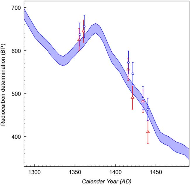
Figure 1 14C dates obtained on earlywood (blue circles) and latewood (red triangles) plotted against IntCal13. Error bars are the 2σ range. (See online version for colors.)
Earlywood and latewood fractions were obtained using a small round drill-bit to mill away each growth band while the sample was held in a clamp under a binocular microscope. To ensure that no contamination between earlywood and latewood was possible, the first and last part (approximately 0.5 mm) of each seasonal growth fraction was excluded from analysis. Earlywood bands produced an average of 4.84 mg and latewood bands an average of 11.78 mg. This was insufficient for AMS dating as a yield of ~20% was expected from the α-cellulose method. As such, earlywood fractions from consecutive years were aggregated together, as were latewood fractions. This ensured that sufficient material was available for measurement, while also averaging out noise that could be caused by influences highly specific to a single-year or a single tree. Each sample, therefore, is part of a pair of samples, one of which represents the average 14C content of earlywood during the years stated (Table 1), while the other represents the average 14C content of latewood during the years stated (Table 1). For the two pairs tested during the reversal, the years represented by earlywood and latewood do not overlap exactly. This was necessary to ensure that sample size was sufficient, and is unlikely to have a significant impact on the results because each sample within a pair still contains material from at least five of the same calendar years (Table 1). As such, it will be possible to establish whether a difference in 14C content exists between earlywood and latewood during this period.
Table 1 Results obtained on earlywood and latewood fractions.

The samples were processed to α-cellulose using a variation on the Jayme-Wise method (Green Reference Green1963) whereby each sample was treated for 24 hr with NaO2Cl, followed by treatment with HCl, 17.5% w/v NaOH, then HCl again (Staff et al. Reference Staff, Reyndard, Brock and Bronk Ramsey2014). This method omitted the solvent wash that is usually performed at the beginning of the extraction because previous studies (Rinne et al. Reference Rinne, Boettger, Loader, Robertson, Switsur and Waterhouse2005; Southon and Magana Reference Southon and Magana2010), as well as our own experiments, have shown that this step does not improve the purity of the α-cellulose. The α-cellulose samples were then combusted and graphitized before being analyzed on the AMS (Dee and Bronk Ramsey Reference Dee and Bronk Ramsey2000; Bronk Ramsey et al. Reference Bronk Ramsey, Ditchfield and Humm2004).
RESULTS
The 14C dates are shown in Table 1 and plotted against IntCal13 (Reimer et al. Reference Reimer, Bard, Bayliss, Beck, Blackwell, Bronk Ramsey, Buck, Cheng, Edwards and Friedrich2013) in Figure 1. In all cases the earlywood samples show older 14C ages than the latewood. As discussed above, a difference that was due solely to the storage and remobilization of carbon would result in the earlywood producing older dates than the latewood when the overall production rate was increasing, and younger when it was decreasing. The fact that the earlywood is older on both the reversal and steep downslope of the curve indicates that an atmospheric effect is also present. This is most likely the result of the seasonal influx of 14C occurring after the start of the growing period, such that it is incorporated into the latewood but not the earlywood. As a result, more 14C is incorporated into latewood than earlywood meaning that latewood appears younger.
Across the years sampled the average difference between the earlywood and the latewood was 26±15 yr. Although this is not quite significant at a 2σ threshold (1.7σ) there is a 96% probability that the latewood has a higher 14C level than the earlywood. It is also highly suggestive that the shift is in the same direction on all 6 pairs with just a 1.6% likelihood of this occurring by chance (calculated as 0.56). The average difference was also calculated for those dates obtained on the reversal and high production parts of the curve. This shows that the seasonal difference is significantly larger when 14C production is high, with an average difference of 33±19 yr calculated for this part of the curve, with a 96% probability that the latewood is more enriched in 14C. For the period in which atmospheric 14C concentration is decreasing a difference of only 12±26 yr was calculated with a 68% probability that the latewood has a higher 14C content and a 32% probability that the relationship is reversed.
DISCUSSION
Roth and Joos (Reference Roth and Joos2013) used 14C and CO2 records to construct a model of 14C production throughout the Holocene. This included estimates of the annual production rate needed to give pre-industrial 14C concentrations after accounting for fluxes between the atmosphere, land, and oceans. During the decreasing portion of the calibration curve for the period of our study, their estimate for annual 14C production is approximately 440 mol yr–1 while during the high production portion it is approximately 540 mol yr–1. This is a difference in production rate of 18.5% between the different portions of the curve. In contrast, the difference between the measured offset on each part of the curve (12 yr and 33 yr) is 63.6%. Because the difference in measured offset between each part of the curve is not proportional to the difference in production rate on each part of the curve, there is likely some factor other than the changing concentrations of atmospheric 14C, which is contributing to the observed offset. As discussed above, this is likely the deposition of stored carbohydrates, which in combination with atmospheric variations, results in the measured offset between earlywood and latewood.
It is possible to calculate the contribution of storage and atmospheric variation to the observed seasonal offset (δ) which is defined as the measured 14C age of latewood subtracted from the age of the earlywood. For any section of the calibration curve this will be given by the following equation:
 $$\delta {\equals}as{\plus}bp$$
where s is the slope of the calibration curve and is unitless, p is the production rate (mol yr–1), a is the influence of storage in years and b is the atmospheric influence in yr2 mol–1. Storage remobilizes carbon from previous years so is influenced by the slope of the curve, i.e. the production rate in previous years, whereas the atmospheric effect is proportional to the production rate in the given year. For the atmospheric influence the years represented by b and p are not identical as those in p represent calendar years whereas those in b are 14C years. Both, however, represent time and as such the equation balances dimensionally.
Because we have measured the seasonal offset in two parts of the curve where the production rate is estimated at 440 mol yr–1 and 540 mol yr–1 (Roth and Joos Reference Roth and Joos2013), it is possible by calculating the slope of the curve in each of these parts to use two simultaneous equations to solve for the constants a and b . During the period of low production, the gradient is calculated as 1.9 and during the period of high production it is calculated as –3.1. Substituting these values into the simultaneous equations gives values of –3.4 yr and 0.042 yr2 mol–1 for a and b respectively. This means that on the low production part of the curve (rising 14C age) the contributions to the offset are –6.5 yr from storage and 18 yr from atmospheric effects for a total offset of 12 yr as measured. During the high production part of the curve (falling 14C age) the offsets are 10 yr from storage and 23 yr from atmospheric effects for a total offset of 33 yr as measured.
Uncertainty is introduced to the estimates for a and b due to the measurement uncertainty ( σ ) in δ . We can utilize this to calculate error estimates for a and b , which in turn gives an approximation of the variation in atmospheric and storage contributions to the observed offset. This is achieved by taking the first-order Taylor series expansion of both a and b with respect to the measurement uncertainty and provides values of –3.36±6.65 and 0.042±0.031 for a and b respectively. The contribution of the variation in storage and of atmospheric variation to the observed offset during the period of reversal can then be calculated at –6.5±13 yr and 18±13 yr, respectively. During the period of high 14C production, the contribution of atmospheric variation is 23±16 yr and the contribution of storage is 10±21 yr.
These errors in a and b are correlated, a must be either negative, which implies storage contributing to the offset, or zero, which indicates no storage. If a is set to zero then it is possible to calculate an alternative estimate for b as 0.049±0.032. This result is obtained by taking the error weighted mean of b in each distinct part of the curve when b=δ/p and the error is given by σ/p. This results in an estimated atmospheric contribution of 26±16 yr during the period of high 14C production and 22±13 yr during the reversal.
Overall, although a seasonal offset cannot be confirmed at the 2σ confidence level, the results obtained suggest that the existence of a true seasonal offset is likely; additional, more precise 14C 14C may confirm this. The results also demonstrate that a seasonal offset will be the product of both stored carbohydrates within the tree and variations in atmospheric 14C levels. The model above produces realistic estimates for the contribution of each of these physiological and atmospheric factors to an overall offset. The error estimates obtained are, however, relatively wide and future work may help narrow these. It should be noted however that the exact scale of the effect seen here may be specific to this particular tree (including its local environment and the health of the specimen) and so we should not expect these parameters to be constant across the region for this species. The key point here is that such effects do seem to be found in some trees.
The presence of these distinct physiological and atmospheric signals in tree rings should be considered in any effort to construct a single-year calibration curve. This physiological signal indicates that deciduous species—and ring porous species such as oak—are not ideal for single-year calibration because of the deposition of stored carbon in their earlywood. Instead, evergreen species that require less of a “kick start” at the beginning of the growing season are more appropriate. Of course, much of IntCal13 has been constructed using oak from Ireland and Germany (Reimer et al. Reference Reimer, Bard, Bayliss, Beck, Blackwell, Bronk Ramsey, Buck, Cheng, Edwards and Friedrich2013). This is not to suggest that the current curves are inadequate for routine calibration of 14C dates, but instead is meant as a caution when high resolution dates on tree rings are being undertaken and a suggestion that latewood be used in preference to earlywood.
Additionally, seasonal variation in the amount of atmospheric 14C has been identified in the tree rings measured. A likely explanation for this is the timing of the annual influx of 14C from the stratosphere into the troposphere. As mentioned above, the phase relationship between this injection of 14C and the growing season of trees has previously been used by Kromer et al. (Reference Kromer, Manning, Kuniholm, Newton, Spurk and Levin2001) to explain incorrect wiggle matches between Anatolian tree-ring sequences and IntCal. These authors argue that the different growing seasons in Anatolia and temperate Europe result in an offset between the two regions, which can be magnified by rapidly changing levels of atmospheric 14C and by climatic factors that affect when growth starts. The explanation offered for the results reported in this paper is that the injection of 14C takes place after formation of earlywood so that more 14C is incorporated into the latewood and it records a younger 14C age than earlywood. This is consistent with the magnitude of the seasonal offset that was observed. During the period of reversal, the production rate was 440 mol yr–1 and a difference between earlywood and latewood of 18 yr due to atmospheric variation was calculated, whereas during the period of high production the rate was 540 mol yr–1 and a difference of 23 yr was calculated. This shows that when the seasonal influx is larger, the difference between earlywood and latewood is also larger.
These results have several significant implications. Firstly, they provide a potential explanation for the incorrect wiggle matches observed by Bayliss et al. (Reference Bayliss, Marshall, Tyers, Bronk Ramsey, Cook, Freeman and Griffiths2017) in medieval period wood from England if the proportion of earlywood to latewood was different in their samples compared to the tree rings used in the construction of IntCal. Secondly, they demonstrate the already mentioned point that deciduous species such as oak might be inappropriate for the construction of a single-year calibration curve when both earlywood and latewood are measured together. Finally, they suggest that short-term atmospheric events (e.g. Miyake events) could be more easily identified in latewood than earlywood, and that measuring only latewood may allow a better estimation of the magnitude of these events and enable events of a smaller magnitude to be identified.
It is important to note again (as was stated above) that these differences are the case only for the single tree that has been measured. Other trees and samples will have grown under different conditions so may have experienced different atmospheric conditions during their growing period. Additionally, physiological variation between trees may mean that storage plays a greater or lesser role in individual samples. This point is significant in terms of the construction of a single-year calibration curve as it will be necessary to assess the extent to which geographic variations are present in annual atmospheric 14C fluctuations. The significant short-term fluctuations discovered by Miyake et al. (Reference Miyake, Nagaya, Masuda and Nakamura2012, Reference Miyake, Masuda and Nakamura2013) have been identified in trees worldwide, but this may not be the case for smaller variations. If annual variations in atmospheric 14C do show geographic variation, it may not be possible to utilize a single calibration curve for each hemisphere as is current practice. Establishing this will require significant effort and resources as multiple trees will need to be assessed in multiple different locations. The results presented here do not demonstrate the presence of geographic variation in 14C content, but highlight the necessity of further investigation into the seasonal signal and variations between different trees.
CONCLUSIONS
The construction of a single-year calibration curve may enable significant improvements in the accuracy of 14C dates obtained from high-resolution samples such as tree rings. Any attempt to do this, however, will need to take note of the intra-seasonal variability that tree rings display. This manifests both in atmospheric changes and in the deposition of carbon that has been stored from previous years. This study has demonstrated that these factors can be separately identified and measured. This both complicates matters in that tree rings may not represent a single-year’s carbon, but also offers opportunity in that atmospheric variability of a smaller magnitude can be identified.
ACKNOWLEDGMENTS
We thank the Natural Environment Research Council for support of the facility at the Oxford Radiocarbon Accelerator Unit. We also thank the reviewers and associate editor who contributed helpful comments to this manuscript.