NOMENCLATURE
- CFD
Computational Fluid dynamics
 $C_H$
$C_H$Stanton number
- D
base diameter (mm)
- DAQ
Data acquisition
- DRDL
Defence Research and Development Laboratory
- h
enthalpy (MJ/kg)
- inf
free stream condition
- M
Mach number
- NI
National Instrument
- P
pressure (bar)
- PCB
Pico CoulomB
- q
(t) local surface heat transfer rate
- ${Q}_{o}$
heat transfer rate at nose (W/cm2)
- ${R}_{n}$
nose radius
- s
distance along the surface of model (mm)
- T
temperature (K)
- TPS
Thermal protection system
- w
condition behind the shock wave
- $\alpha$
angle-of-attack
- $\theta_{c}$
cone deflection angle
- $\alpha$
angle of rotation
- $\rho$
density (kg/m3)
- 0
stagnation condition
- 2
condition behind the incident shock wave
- 5
condition behind the reflected shock wave


1.0 INTRODUCTION
Testing of models in hypersonic flow is essential to quantify the heat transfer rates on a vehicle configuration to design the thermal protection system (TPS) for space missions. Carefully designed ground-based investigation plays an important role in providing design data as well as insights into the unknown aspects of flow physics. In addition, it will be very useful to design the TPS for a space mission. The shock tunnel is a powerful short duration impulse facility that can produce total energy content of flow in addition to flow Mach number and Reynolds number in a hypersonic flight regime. The major limitation of this impulse facility is the ultra-short test duration in the order of 3ms. In shock tunnels, reservoir conditions are obtained by the formation of compression waves in the driven section. The probable variation in free stream test condition for every shot is approximately  $\pm 5 -- 15\%$[Reference Niranjan, Saravanan, Jagadeesh and Reddy1]. Moreover, it is hard to ensure the comparable test flow spectrum over the cone model during the experiment for every test condition in shock tunnel facilities. Model sizing and support structure are important considerations for designing the vehicle because of the blockage effect.
S Saravanan et al.[Reference Saravanan, Jagadeesh and Reddy2] carried out experiments on missile frustums flying at hypersonic speed. The effect of fins on the surface heating rates of missile-shaped body also is investigated. The tests are performed at the flow Mach number of 5.75 and 8 at a stagnation enthalpy of 2MJ/kg. The measured heat transfer rate along the surface with fin shape is slightly higher than that of a model without a fin. Aerobraking[Reference Raju and Craft3] is the best maneuver that can decelerate upon entry from the planet’s atmosphere. These aerobraking maneuvers result in substantial savings in the propellant for a space mission and permits installation of a larger payload. To minimise the effect of aero heating, the hypersonic vehicle must have a very blunt nose. M Ibrahim and K P J Reddy[Reference Mohammed Ibrahim and Reddy4] investigated heat transfer measurement using platinum thin-film sensors on large angle blunt cones entering the Martian atmosphere. L Jian-Xia et al.[Reference Jian-Xia, Zhong-Xi, Xiao-Qian and Jun-Tao5] measured the heat flux distribution on a blunted wave rider, including the effect of angle of attack and sideslip angle. For an angle of attack lower than  $10^{\circ}$, the heat flux coefficient on the leeward surface is lower than 0.15. Over the years, several heat transfer measurements on a blunt cone model have been reported in the open literature (Steward and Chen[Reference Stewart and Chen6], Srinivasan et al.[Reference Srinivasan, Desikan, Saravanan, Kumar and Maurya7]).
Thin-film resistance thermometer [Reference Miller8,Reference Wannenwetsch, Ticatch, Kidd and Arterbury9], coaxial surface thermocouple[Reference Kidd10], and null-point calorimeter[Reference Kidd, Jag and Richard11] are the temperature sensors used in transient conditions. S R Sanderson and B Sturtevant[Reference Sanderson and Sturtevant12] developed and tested a new form of surface junction thermocouple sensor in which the response time of heat flux gauge is  $1 \mu s$ and is suitable for measuring large transient heat fluxes in hypervelocity wind tunnels. J P Hubner et al.[Reference Hubner, Carroll and Schanze13] examined the development and application of high-speed imaging and luminescent-coating techniques to measure the full-field surface-heat transfer rates. There are many other techniques such as thermal paints[Reference Asai, Kunimasu and Iijima14], infrared thermography[Reference De Luca, Cardone, Carlomagno, Aymer de la Chevalerie and de Roquefort15], and thermographic phosphors[Reference Micol16] that are used to view the thermal imaging of the full field. In the present investigation, platinum thin-film sensors are used to measure the convective heat transfer rate. The deposition of platinum thin film on the substrate can be done by a hand-painting technique or a vacuum-sputtering technique. Most researchers developed the heat flux gauges through a platinum paint technique[Reference Kumar17-Reference Menezes, Saravanan, Jagadeesh and Reddy20]. The main drawback of the hand-painting technique is the difficulty in controlling the thickness and uniformity of the film. To satisfy the 1D heat transfer theory, the measuring surface film should have a negligible effect on the heat conduction. Although the platinum thin film thickness is very small, there is an effect on the surface temperature history that should be considered. As the thickness of the film increases, its thermal capacitance increases. The increase in thermal capacitance leads to an error in the measurement. In vacuum-sputtering techniques, precise control on the thickness of thin film is possible. In this research paper, advanced techniques like vacuum sputtering and vacuum deposition of thin-film platinum are used for fabricating the heat transfer gauge. Details of platinum thin sensors, tunnel results, and the comparison of measured value with theoretical results are described in this article. A detailed review of advanced measurement techniques is given including gauge calibration, data reduction techniques, and uncertainty analysis. The experimental investigation of surface pressure and heat flux using a thin-film technique on a hypersonic vehicle at a high enthalpy condition is inadequate in open literature. To fill this gap, we have initiated an investigation using a hypersonic shock tunnel facility at the Defence Research & Development Laboratory (DRDL). The prime objectives of the present study are (1) to observe the shock pattern which envelops the blunt cone model at hypersonic speed, (2) to measure and investigate the stagnation, surface heat transfer, and surface pressure distribution for a blunt cone model at
  ${0}^\circ and {5}^\circ$ angle of attacks, (3) to compare the blunt cone heat transfer and surface pressure distribution values with a sharp cone model at approximately the same flow conditions, and (4) to validate the experimental results with a well-known simple theroretical prediction and Computational Fluid dynamics (CFD) simulations.
2.0 FACILITY DETAILS
Shock tunnels are ground-based test facilities that are used to simulate high-speed flows for a short period of time. The shock tunnel facility consists of a shock tube, convergent–divergent nozzle, and a test section and dump tank as illustrated in Fig. 1. The total length of the shock tunnel was 31.7m. The lengths of the driver section and the driven section were 5m and 18.7m, respectively, and both were made of stainless steel. The shorter section and the longer section were separated by an aluminum diaphragm that had a thickness of 6.4mm, groove depth of 2.8mm, and groove length of 200mm. Similarly, the shock tube and the C-D nozzle were separated by a Mylar diaphragm. The driven section and the test section and dump tank were evacuated from 1bar to 0.5bar and  $1 \times {10}^{-6}$mbar, respectively. Upon the diaphragm getting ruptured, the shock wave would get transmitted through the driven section which in turn would increase the static pressure and static temperature across the shock wave. Upon reaching the end of the shock tube, where the Mylar diaphragm is placed, the moving shock would get reflected rupturing the Mylar diaphragm due to the high-pressure flow. Thus, instantaneous high pressure would be generated by the moving incident and reflected shock waves in the shock tube. This high-pressure and high-temperature air, ahead of the just ruptured Mylar diaphragm, was almost at zero velocity, and acted like a settling chamber. These test gases expanded through the convergent divergent nozzle and produced a hypersonic Mach number flow. The conventional shock tunnel in DRDL could produce a maximum stagnation enthalpy of 3MJ/kg. However, in this present investigation, the tunnel was operated at a stagnation enthalpy of 1.4MJ/kg with a stagnation pressure of 30bar. A nozzle exit diameter of 590mm was used for generating a Mach number from 6 to 7[Reference Shanmugam, Rampratap and Prasad21].

Figure 1. Layout of hypersonic shock tunnel.
3.0 TEST MODEL
In the present investigation, both blunt cone and sharp cone models were used for the vehicle configuration. The cone model has an apex angle of  $11.38^{\circ}$ and a base diameter of ‘D’ as illustrated in Fig. 2a and 2b. The nose radius of the blunt cone model was 0.2 D as shown in Fig. 2. The test model size was designated based on the following constraints: (1) the effect of blockage ratio, (2) interaction of aerodynamic flow field between all boundary layers and the cone model, (3) substrate thickness of thin-film sensors, (4) effect of the free stream Reynolds number based on the length of model, and (5) model support system. The test models were fabricated with aluminum alloy due to its light-weight nature, and the mass of the test model configuration was kept approximately at 5 kg. GS2 and GS3 were nose sensors. GS2 was located along the axis of the model and GS3 was placed on the cone model at an axial distance of 1.9mm from GS2. One half of the model had platinum thin-film sensors that were labeled from G1 to G6. The other half of the model had pressure sensors, and these were labeled from S1 to S6.
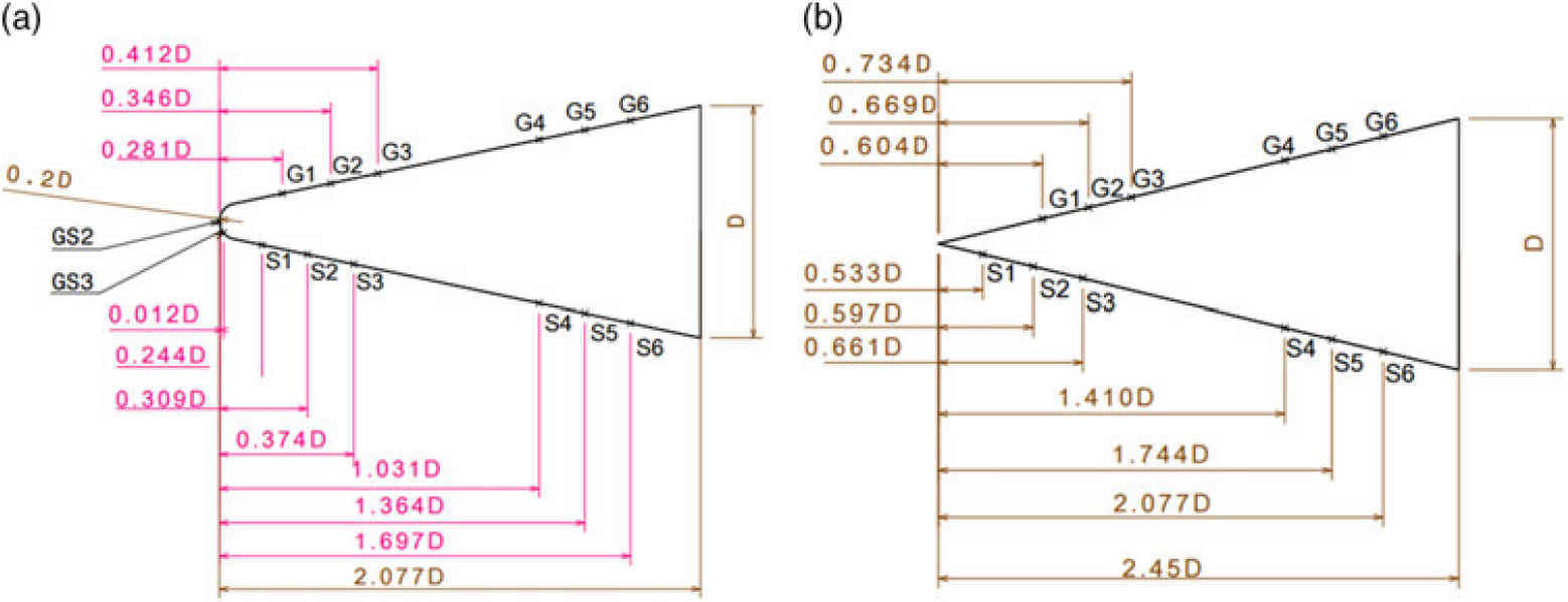
Figure 2. (a). Blunt cone model used for experiments (Note: D = 150mm); (b) Sharp cone model used for experiments (Note: D = 150mm).
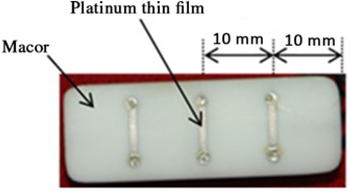
Macor, Pyrex, and quartz are used commonly as substrate because they are thermal insulators. In the present case, Macor was chosen as a substrate because it has superior properties over all the other materials. It can withstand a temperature of  $1,000^{\circ}$ without any deformation, and it is more easily machinable than the other ceramic materials like Pyrex and quartz. In addition, it also satisfies the semi-infinite slab assumption. The thermal penetration depth of Macor is inversely proportional to the square root of thermal diffusivity. Materials with lower diffusivity (such as Macors) have longer semi-infinite test times, whereas high diffusivity materials (such as metals) have shorter semi-infinite test times[Reference Kinnear and Lu22]. Silicon carbide paper (C-320 grade) was used to get a better polished surface on the Macor. Then, the polished surface was cleaned with acetone using an ultrasonic cleaner to avoid contamination. Two holes of 1mm diameter were drilled on the Macor to provide electrical connections for the gauge. The electrical wire with an outer diameter of 0.6mm was used for the electrical connection. A silver paste of EPOTEX was applied between the electrical wire and the thin film gauge ends. It was cured at
  $150^{\circ}$ for 15 minutes.
3.1 Thin-film technique
A commonly used heat flux measurement technique involves a thin layer of film deposited in the Macor substrate. Platinum, tungsten, nickel, silver, copper, and gold are thin-film materials. Platinum has good quality resistivity. It provides moderately linear and steady output. Platinum is inert to hostile environments compared to other thin film-conducting materials. In the present investigation, platinum was chosen as the thin-film material. Thin-film technique can be done by either hand painting or vacuum sputtering. Before the sputtering process, Kapton tape was masked on the substrate so that the thin layer was open for platinum deposition. To get uniform resistance over the thin film, the substrate was placed in the effective sputtering area. The value of resistance lays between 50 and 100ohms. The thickness of the thin film of platinum was  $0.4 \mu m$ depending upon the area of the thin film, the resistance, and the resistivity of the thin film. After the deposition of thin film, gauges were placed in the muffle furnace and then the temperature was increased up to
  $800^{\circ}$. This temperature was maintained for about 30 minutes to improve the bonding strength between the substrate and the thin film. Then, leads were made for giving excitation current to the gauge to measure the output voltage during the test. Both rectangular and circular Macors were used for heat flux measurement. In the rectangular Macor, a 10mm distance was maintained between the thin-film gauges and between the substrate end of both sides and the thin film gauges. Figure 3 illustrates a photograph of the heat flux gauge.

Figure 3. Heat flux gauge used for present study.
3.2 Calibration of thin film
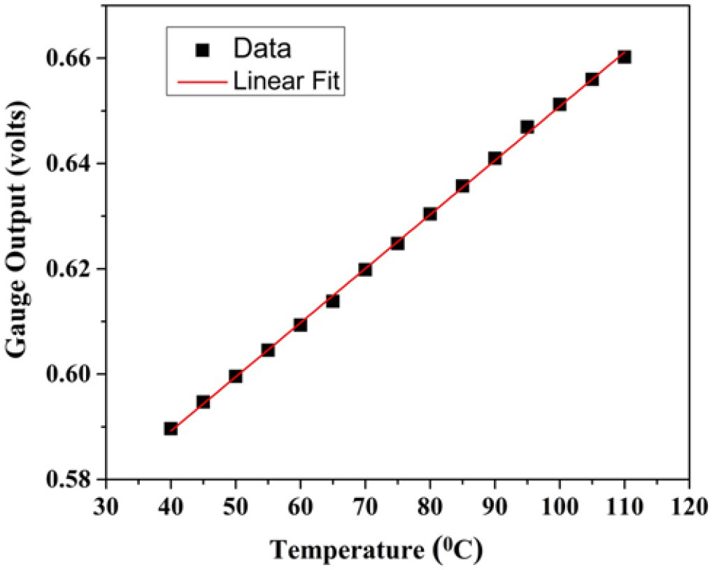
The purpose of alpha calibration is to determine the sensitivity and linearity of the gauge. The set up consisted of the heating mantle, empty beaker, oil-filled beaker, and digital thermometer. The oil-filled beaker was placed on the heating mantle. Oil was chosen as the medium since it is a good heat transfer medium and has a high boiling point. Heat flux gauges and temperature sensors were placed in an empty beaker. The gauges were energized with a constant power supply of 20mA. Calibration was performed by increasing the heat input from  $40 to 110^{\circ}$, and allowing the gauges to cool from
  $110 to 40^{\circ}$. Gauge temperature was measured every
  $5^{\circ}$ with the corresponding output voltage being measured from National Instrument (NI)-based data acquisition system. Hence, calibration data were considered during the cooling cycle for accurate results. The variation of the gauge output voltage with temperature gives the sensitivity of the gauge as shown in Fig. 4. For all heat flux gauges, the sensitivity varies from
  $1.03 to 2.45mV/^{\circ}C$. The value of the thermal product (
 $\beta$) depends on density, specific heat, and thermal conductivity of the backing material. Its typical value is
  $1705W-{s}^{1/2}/{{m}^{2}}-K$.

Figure 4. Typical calibration curve.
3.3 Dynamic response test
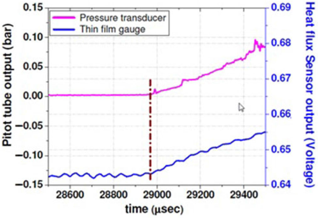
The heat flux gauge was mounted adjacent to the pitot pressure probe at the same axial location from the nozzle exit (Fig. 5). The data from both sensors are acquired at the same synchronous sampling rate. The difference in the rising instants of both sensors gives the response time. From Fig. 6, it can be observed that the thin-film gauge responded at the same time as the pressure transducer. This response time indicates that the thin-film gauge has dynamic characteristics like the pressure transducer. The sensitivity of the pitot tube used for the present study is 1467mV/bar.

Figure 5. Probe arrangement for dynamic response test. (Note that all dimensions are in mm.)

Figure 6. Dynamic response test result.
4.0 TEST CONDITION
Experiments were carried out on the cone model at  $\alpha = 0^{\circ}$ and
  $5^{\circ}$ at M = 6.56 with angle of rotation of
  $0^{\circ}, 90^{\circ}$, and
  $180^{\circ}$ in both angles of attack. The time required for the flow to cover the model length of 2.077 D for a free stream velocity of 1.6km/s would be 0.194ms. The uniform flow over the model was more than two times, so the model length was adequate for the tunnel operation. In the first test, the heat flux gauges were on the top surface of the model and the pressure ports were on the bottom portion of model. Then, in the second test, the model was oriented
  $180^{\circ}$ by the same incidence with the same condition to get the data in the other half of the model. Approximately 12 runs were carried out for different angles of attack. After a couple of tests, the resistance of the gauges was examined for the durability of the platinum thin-film gauges. It was found that the variation of resistance was very minor indicating that sputtered sensors had longer durability. Experimental investigation was carried out in a low enthalpy condition (
 $\sim 1.4MJ/kg$) to minimize the uncertainty. Table 1 gives the test condition of the hypersonic shock tunnel and its uncertainty inside the bracket. The dynamic pressure of the atmosphere and flight Mach number corresponds to an altitude of approximately 30km[Reference Heiser and Pratt23].
Table 1 Nominal test condition during the present experiment

4.1 Data reduction techniques
The Cook–Felderman technique[Reference Cook and Felderman24] and the Kendall–Dixon technique[Reference Kendall, Dixon and Schulte25] are analytical methods that are based on the assumptions of heat conduction to a semi-infinite solid (Macor) with constant thermal properties being used to derive closed-form solutions and to obtain the heat flux. The 1DHEAT data deduction code[Reference Hollis26] can be used to compute the heat-transfer data. The Cook-Felderman algorithm converges to a value very close to the theoretically calculated stagnation-point heat-transfer value of  $62.5W/{cm}^{2}$. The Cook-Felderman algorithm proved useful for calculating the heat-transfer rate from data where the random noise has been removed. The predicted stagnation-point heating-rate value exceeds the other two schemes (the Kendall–Dixon technique and the 1DHEAT data-deduction code) and the difference is about 19 and 22%, respectively. This difference could be a noise present within the data, and the sharp fluctuations in the response data caused large errors in the calculated heat-transfer rate. In the present investigation, data extraction from the Cook–Felderman technique is used. The number of sampling points recorded, amplification factor, sensitivity of the heat-flux gauge, and thermal product of material are given as inputs to convert voltage time history to heat flux. The accuracy of the calculated heat flux depends on the time-step size. The time step used is
  $1 \mu sec$, which is the same as that of the Data acquisition (DAQ) sampling time step. The voltage–time history obtained from platinum thin-film gauges is numerically integrated by the Cook–Felderman technique to measure the convective heat transfer rate (Figs 7 and 8). The parabolic fit data is used for numerical evaluation of the heat flux since part of the signal represents the steady heat flux to the body.

Figure 7. Unsteady Voltage-time history obtained from platinum thin film sensors for heat flux gauge GS2.

Figure 8. Typical heat transfer signal obtained from numerical integration of Voltage-time history.
The measured heat-transfer rate over the blunt cone model should ideally remain constant with time. This ideal situation requires the free-stream flow quantities to be constant with time during the tunnel operation. In the hypersonic shock tunnel, the probable variation in free-stream properties does exhibit with respect to time, especially in the case of air being used as test gas. Therefore, a time-averaging procedure was adopted to obtain the measured heat-transfer rate over the blunt cone model.
4.2 Numerical study
The steady-state flow field around the blunt cone model was simulated using the Ansys Fluent code. The Navier- Stokes (NS) equation would be desirable to estimate the heating rates and other relevant flow field and to solve the complete flow field on the models. The Fluent NS code can handle incompressible and compressible flow problems for steady and unsteady flow regimes. The SST k-omega turbulence model was used for the CFD simulation. The structured mesh with finer grids near the walls was used to capture the shock pattern. The various boundary conditions used in the study are as follows: Inlet: The free-stream conditions obtained at the inlet of the test section in the shock tunnel that were specified in the computational domain. The flow properties such as static pressure of 840Pa, static temperature of 154K, and flow Mach number of 6.56, which were used for the CFD simulation. Outlet: At the outlet of computational domain, all variables were extrapolated from interior domain. Wall: Blunt cone model surfaces were used as a wall boundary condition. No-slip condition and constant temperature of 300K were stated as wall boundary conditions. The target residuals to terminate the simulation were set at  $1 \times {10}^{-5}$. In the initial simulations, the multi block body-fitted grid used for the computations has a total number of around 9,67,835 elements. In the subsequent runs, the number of grid points has been increased (i.e., grid refinement study) to check the variations in heat-transfer rates and surface pressure along the model surface. Very close to the test model surface, finer structural mesh has been used for gradient accuracy. Initial simulation has been carried out with an implicit first-order accurate numerical scheme and the final simulation was carried out with a high-resolution second-order accurate scheme. The target residuals to terminate the simulation have been set at
  $1 \times {10}^{-5}$. Computed surface heat-transfer rate and surface pressure along the surface of blunt body for three different grids (9,67,835, 16,69,394, and 28,45,628 elements) are used. It was seen that the changes in the calculated parameters for different grids were within
  $\pm 2.5\%$. Finally, total number of around 16,69,394 elements have been chosen for the present investigation. Numerical simulation was carried out for the
  $0^{\circ}$ and
  $5^{\circ}$ angles of attack to compute the heat transfer and the pressure distribution on a blunt cone model.
5.0 RESULT AND DISCUSSION
5.1 Schlieren photographs
The test model was carefully placed at the center of the test section to observe the detached shock structure clearly. The time-resolved schlieren images around the blunt cone model at a  $5^{\circ}$ angle of attack are shown in Fig. 9. The detached shock wave around the cone model is observed by Schlieren techniques. The high-speed camera is capable of recording 1,000 frames per second with a maximum resolution of
  $1,632 \times 1,200$ pixels. The pixel resolution gets reduced to
  $64 \times 64$ pixels at 1,44,175 frames per second as the recording speed increases. In the present investigation, a high-speed camera was used for capturing Schlieren images at
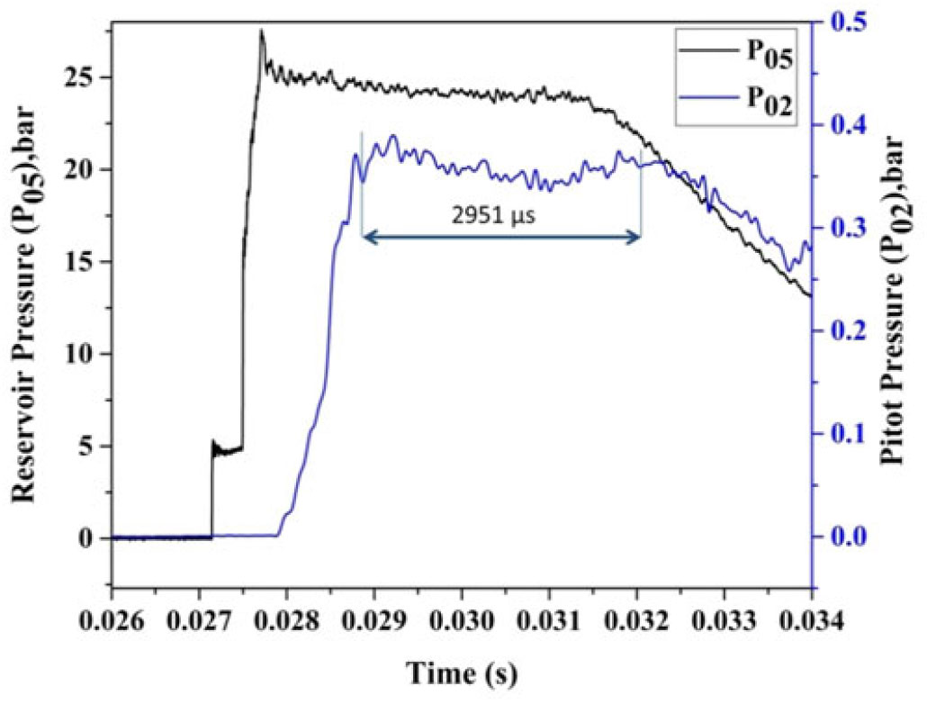
  $384 \times 240$ resolution and 14,035 frames per second. The time-scale variation of the reservoir pressure (
 $P_{05}$) along with test section pitot pressure (
 $P_{02}$) is shown in Fig. 10.

Figure 9. Time-resolved sequential Schlieren images during steady time.

Figure 10. Variation of reservoir pressure along with pitot pressure variation with respect to time.
According to Fig. 10, the measured pitot pressure reaches  $2,951 \mu s$, but from the sequential Schlieren images, the shock structure remains unaltered for about
  $7,860 \mu s$. This outcome could be explained with reference to Fig. 11 that shows the variation of stagnation pressure ratios (
 $P_{02}/P_{05}$) with respect to time. This pressure ratio is a unique function of Mach number and the specific heat ratio that keeps the flow remaining steady for
  $7,860 \mu s$. As a result, the Mach number remains unaltered for
  $7,860 \mu s$. The shock structure being primarily dependent on the free stream Mach number remains invariant during this period (
 $7,860 \mu s$) as seen in the Schlieren images in Fig. 9. After the steady flow, flow properties such as static pressure, static density, and so on start decreasing rapidly due to the decrease in the amplitude of the reservoir pressure.
Figure 11. Variation of stagnation pressure ratio with respect to time.
The shock standoff distance ( $\delta$) is calculated from the density gradient across the shock wave and nose radius of the blunt cone model. The expression for shock standoff distance as given by M Inouye[Reference Inouye27] is as follows:
 $$\frac{\updelta }{{{\rm \ \ R}}_{{\rm n}}}{\rm\ =\ 0.}78\left(\frac{{\uprho }_{{\rm inf}}}{{\uprho }_{{\rm w}}}\right)$$
where  ${\rho}_{{\rm inf}}$ is the free-stream density across the shock wave and
  ${\rho}_{{\rm w}}$ is the density behind the shock wave. The shock stand-off distance is measured using Fiji software[28]. The calculated shock stand-off values correspond to
  $7,624 \mu s$ for comparison. The experimentally measured and the predicted shock standoff distances are 2.06 and 2.29mm, respectively, whereas the shock standoff distance obtained from the CFD simulation is 2.102mm. Thus, the shock standoff distance measured from the Schlieren images matches well with the predicted and CFD simulated values. These results show the validity of the prediction of shock stand-off distance by Equation (1) and conditions used for CFD simulation. The shock layer thickness calculated from the Schlieren images and the results are compared with the CFD simulation for
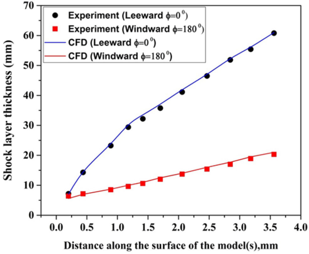
  $\alpha = {5}^{\circ}$ as shown in Fig. 12. As expected, the shock layer thickness is closer on the windward side than on the leeward side at the
  $5^{\circ}$ angle of attack.

Figure 12. Variation of shock layer thickness from the model surface for  $\alpha = {5}^{\circ}$.
5.2 Theoretical estimation of stagnation-point heat transfer
The problem of predicting stagnation-point heat transfer on blunt bodies is reported in the literature[Reference Lees29,Reference Fay and Riddell30]. Fay and Riddell[Reference Fay and Riddell30] first estimated the stagnation-point heat transfer on hypersonic flight where high temperature existed behind the shock wave. Due to its simplicity, this equation is still in use to investigate the thermal field on a hypersonic vehicle. The Fay and Riddell formula was incorporated with the stagnation velocity gradient. The correlated formula for axisymmetric bodies is as follows:
 $$\ {~\dot{{\rm q}}}_{{\rm w}}{\rm\ =\ 0.763}{\left({\rm Pr}\right)}^{-{\rm 0.6}}\ \ {\left({\uprho }_{{\rm 2}}{\mu }_{{\rm 2}}\right)}^{{\rm 0.5}}\frac{{\rm d}{{\rm u}}_{{\rm e}}}{{\rm ds}}\left({{\rm h}}_0-{{\rm h}}_{{\rm w}}\right)~$$
The velocity gradient at stagnation point is predicted from Equation (3):
 $$\frac{{\rm d}{{\rm u}}_{{\rm e}}}{{\rm ds}}{\rm\ =\ }\frac{{\rm 1}}{\sqrt{{{\rm R}}_{{\rm n}}}}{\left[\frac{{\rm 2(}{{\rm P}}_{{\rm 02}}-{{\rm P}}_{{\rm inf}})}{{\uprho }_{{\rm 02}}}\right]}^{{\rm 0.25}}$$
The unknown values in Equation (2) are obtained from normal shock relations at the stagnation point by an iterative method. The term  $R_{n}$ is the nose radius of the blunt cone model. The estimated stagnation-point heat-transfer rate at Mach 6.56 was
  $62.5W/{cm}^{2}$ (Table 2). Numerical simulation was carried out using FLUENT 15.0 to validate the measured value and the theoretical value using the Fay and Riddell formula. The experimentally measured value did not differ much from the theoretical and computational values.
Table 2 Stagnation point heat transfer (W/cm2) for Mach number 6.56 at  $\alpha = 0^{\circ}$

5.3 Zero-degree angle of attack case
Investigation was carried for a flow Mach number of 6.56, and the free-stream Reynolds number based on model length is  $9.1 \times {10}^{5}$. The expected state of the boundary layer along the model length is turbulent. At
  $\alpha = {0}^\circ$, the variation of the heat flux along the surface for the blunt cone and sharp cone model is shown in Figs. 13 and 14 where the experimental results are compared with the computational ones. The heat flux was measured at the top surface of the model (
 $\phi = {0}^\circ$) and the surface pressure distribution was measured at the bottom surface of the model. Then, the model was rotated by
  $180^{\circ}$ at the same incidence with the same test condition to get the data for the other half of the test model. The heat transfer to the body surface is a function of body shape and flight conditions. The maximum surface heating rate occurs at the stagnation point. This result is due to the occurrence of a large amount of kinetic energy dissipation at the stagnation point in the thin shock layer region at hypersonic free-stream velocity. The sudden increase in the temperature across the curved shock wave is proportional to the square of the speed for high-speed flights, which is prominent to high heat-transfer rates to the stagnation point. The velocity gradient is 0 at the stagnation point and increases further due to the 3D relieving effect. The local surface temperature and the heating rate suddenly decrease along the flow direction as seen in Figs. 13 and 14. The experiment could not capture the stagnation-point heat-transfer rate in the sharp cone model due to the unavailability of the material for the gauge fixation.

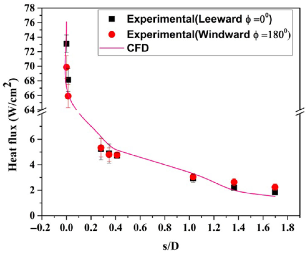
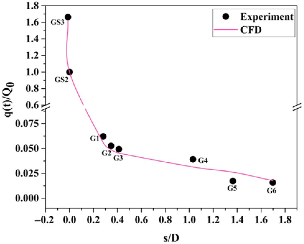
Figure 13. Distribution of convective heat transfer rate over the surface of a blunt cone model at  $\alpha = {0}^{\circ}$ for M = 6.56.

Figure 14. Distribution of convective heat transfer rate over the surface of a sharp cone model at  $\alpha = {0}^{\circ}$ for M = 6.56 [Reference Saiprakash, Senthilkumar, Balu, Shanmugam, Rampratap and Kadamsunil31].
For the same flow Mach number, the decrease in the windward heat transfer rate along the model surface for the gauges G1 to G6 was 60 and 58% for the sharp and the blunt cone models, respectively. Similarly, it was 59 and 65% for the leeward heat transfer rate, respectively. It shows good quality of flow in the shock tunnel and durability of heat flux gauges during the same test conditions.
The sharp cone model experiences higher heating rate along the stream-wise direction compared to the blunt cone model. For the blunt model, when flow approaches at 1.697 D from the nose, the surface heating rate (i.e., as measured by gauge G6) is approximately equal to 2.5% of the stagnation-point heating value. As measured from heat flux gauges G1 to G6 in the leeward and windward direction, the heat flux reduces from 7.5 to 2.5% of the stagnation-point heat transfer. For the blunt cone model, the difference in the measured stagnation heating value above the identical test is 4.4%.
The percentage of reduction in the heat flux for the blunt cone model having a nose radius of 0.2 D, as measured from heat flux gauges G1 to G6 located on the surface of the model, is about 21 to 41% compared to the sharp cone model. Due to a weaker shock strength on the sharp cone model, heating of the air is low and the heating of the body is high. On the other hand, for the blunt cone model, a strong shock wave occurs ahead of the nose where a large dissipation of heating to the air and smaller heating to the body is achieved. This statement is evident from the heat flux measurement.
The patterns of heating rate on the blunt cone and the sharp cone models are almost symmetrical over the top and bottom surfaces at  $\alpha = {0}^{\circ}$. At
  $\alpha = {0}^{\circ}$, the discrepancy in the windward and the leeward heat flux value is within
  $\pm 5\%$ for blunt model and
  $\pm 10\%$ for the sharp cone model. At
  $\alpha = {0}^{\circ}$, the deviation in the windward and the leeward heat flux value occurs mostly because of the irregularity of the groove depth in the aluminum diaphragm and perhaps due to accumulation of moisture in the driver section. In addition to that, a minor Mylar diaphragm fragment could affect the flow quality. Due to this phenomenon, the same quality and quantity of flow could not be produced even though the tunnel was operated at the same test conditions.
5.4 Non-zero-degree angle-of-attack case
The flow becomes more complex at  $\alpha = {5}^{\circ}$ when compared with
  $\alpha = {0}^{\circ}$ due to asymmetry. For a cone model, the streamlines in the flow between shock wave and cone surface are no longer planar; they are curved in 3D space between the shock and the cone surface. For symmetrical bodies, stagnation streamline and maximum entropy occur at the stagnation point. At an angle of attack, the stagnation streamline does not pass through the normal portion of the bow shock wave and maximum entropy does not occur at the stagnation streamline. The stagnation streamline is attracted to the portion of the cone model by the maximum curvature.
At  $\alpha = {0}^{\circ}$, the nose is acting as stagnation point with maximum heat flux, whereas when
  $\alpha = {5}^{\circ}$, the stagnation point shifts to s/D = 0.012. The increase in maximum heat transfer at s/D = 0.012 compared with the nose is 41%. For the blunt cone model, the measured nose heat transfer rate (i.e., heat flux gauge GS2) at
  $\alpha = {0}^{\circ}$ is 1.14 times greater than at
  $\alpha = {5}^{\circ}$. Also, at
  $\alpha = {5}^{\circ}$, the heat flux increases about 50% at s/D = 0.012 (i.e., heat flux gauge GS3) compared with
  $\alpha = {0}^{\circ}$. This result postulates that the distribution of convective heating on the model surface at angle of attack demands the thermal protection system not only at the nose but also at the other parts of the model surface. Figures 15 and 16 show the variation of heat flux distribution with leeward side (
 $\alpha = {0}^{\circ}$) and windward siden (
 $\alpha = {180}^{\circ}$) at
  $\alpha = {5}^{\circ}$ for M = 6.56. At a
  $5^{\circ}$ angle of attack, curved streamlines curl around the body from the bottom of the cone (called the windward surface) to the top of the cone surface (called the leeward surface). At this angle of attack, the windward surface of the cone model is inclined to the flow direction of the hypersonic stream.

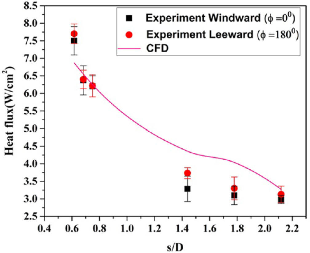
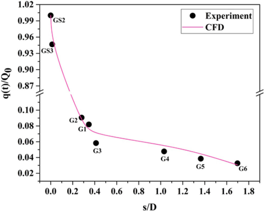
Figure 15. Distribution of the convective leeward heat transfer rate ( $\phi = 0^{\circ}$) over the surface of a blunt cone model at
  $\alpha = 5^{\circ}$ for M = 6.56. (* Heat flux port GS3 at the windward side.)
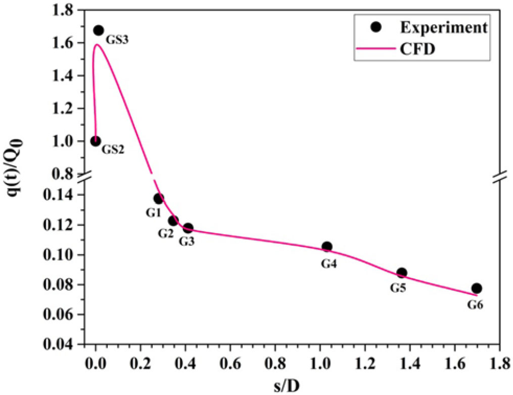
Figure 16. Distribution of convective windward heat transfer rate ( $\phi = 0^{\circ}$) over the surface of a blunt cone model at
  $\alpha = 5^{\circ}$ for M = 6.56.

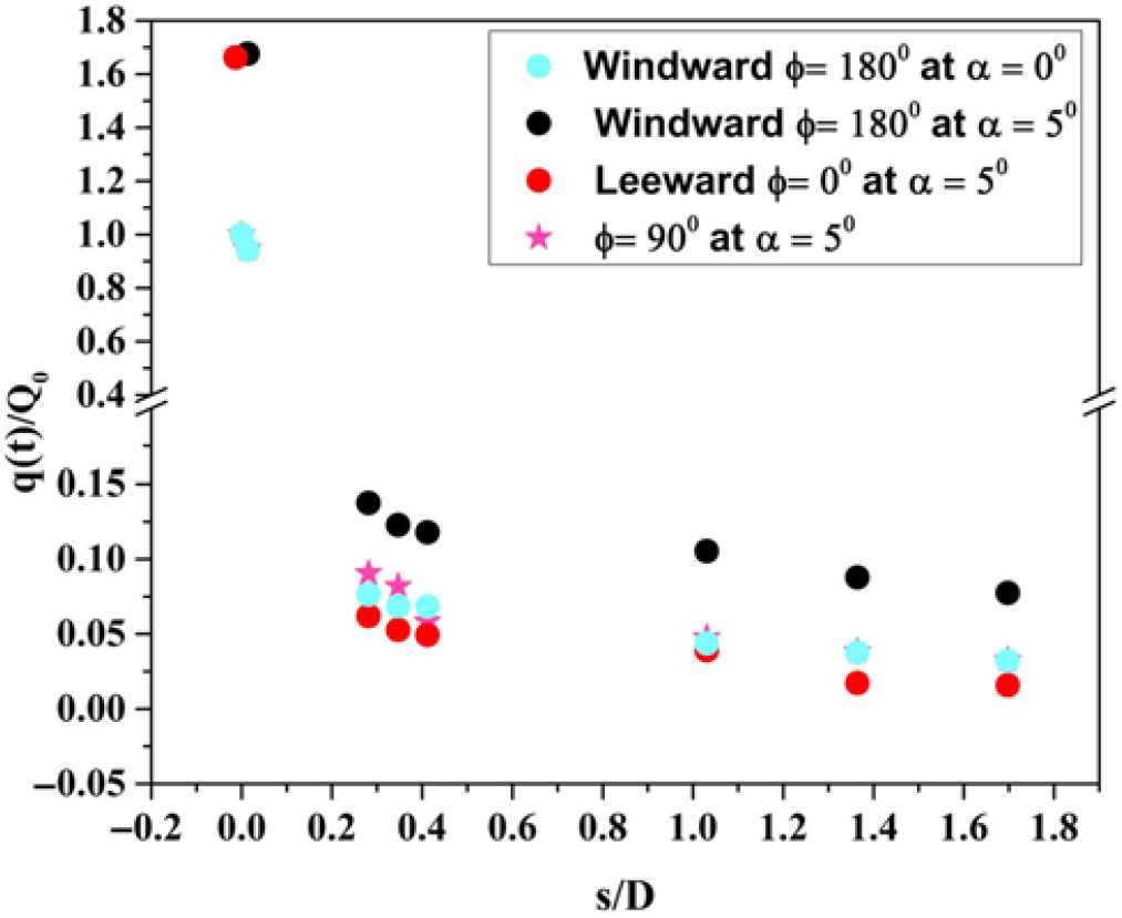
Figure 17. Distribution of convective heat transfer rate ( $\phi = 0^{\circ}$) over the surface of a blunt cone model at an angle of attack of
  $5^{\circ}$ for M = 6.56.

Figure 18. Variation of measured convective heat transfer rate over the surface of a blunt cone model at an angle of attack of  $5^{\circ}$ for M = 6.56.
At  $\alpha = 5^{\circ}$, during the test for
  $\phi = 0^{\circ}$ and
  $\phi = 180^{\circ}$, heat flux gauge GS3 is always located at the windward direction. The difference in measured maximum heating value of the two tests is within
  $\pm$10%.
At  $\alpha = 5^{\circ}$, from s/D = 0.1 to 1.78 (Fig. 12), the shock layer thickness increases in the windward ray (
 $\phi = 180^{\circ}$) from 5.3 to 20.3mm and consequently the surface heating rate decreases along the model surface (Fig. 20). Similarly, in the leeward ray (
 $\phi = 180^{\circ}$), the shock layer thickness increases from 7.1 to 60.7mm for the same s/D distance. Due to the higher shock layer thickness in the leeward ray compared to the windward ray, the surface heating rate is higher on the windward side rather than the leeward side. In addition to that, flow deflection angle and the density ratio also affect the heating rate[Reference Stewart and Chen32].

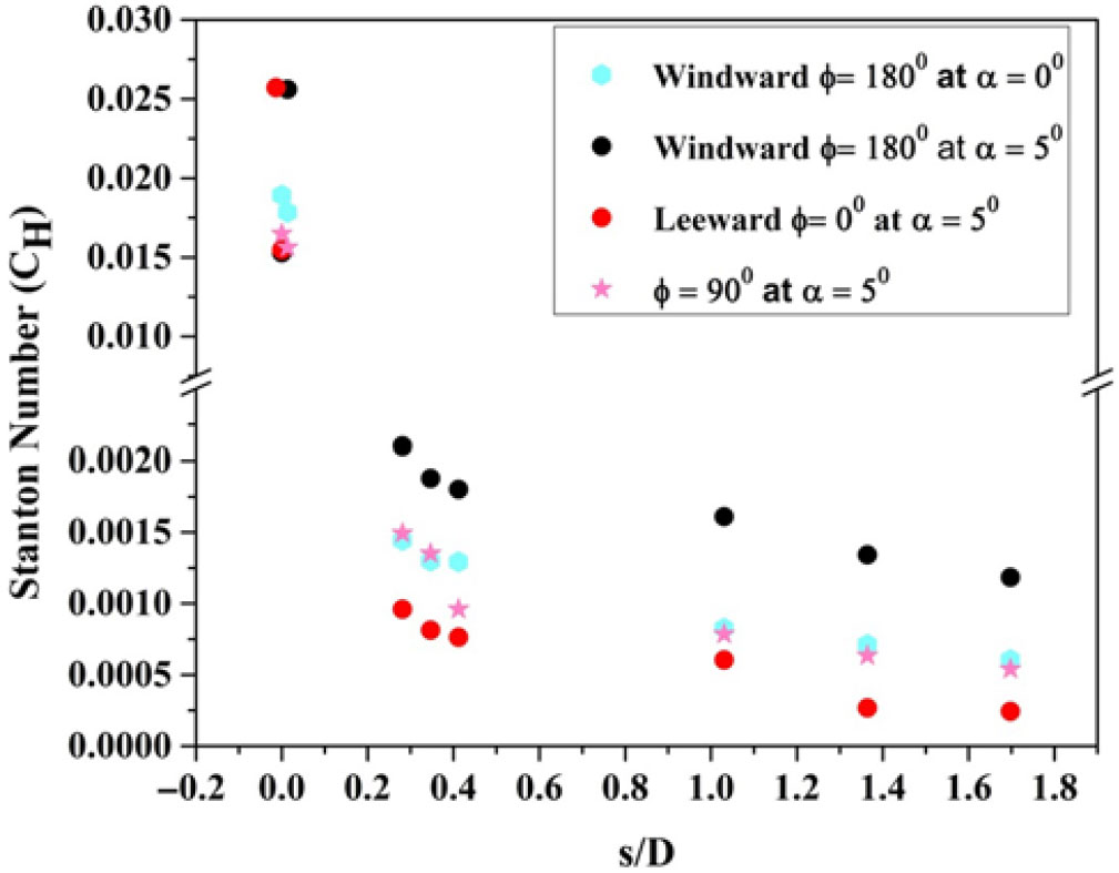
Figure 19. Variation of correlated Stanton number along the surface of a blunt cone model for different angles of attack.

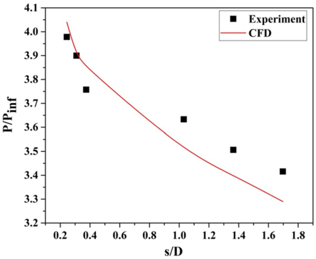
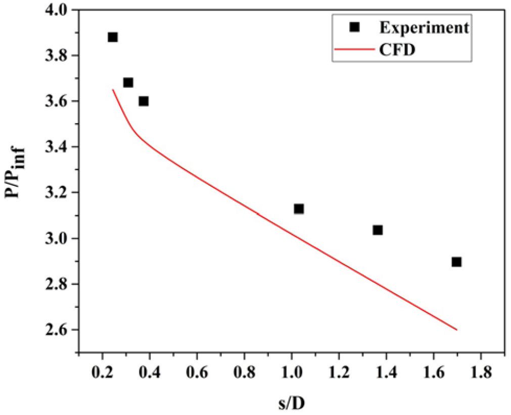
Figure 20. Distribution of surface pressure over the surface of a blunt cone model at  $\alpha = 0^{\circ}$ for M = 6.56.

Figure 21. Distribution of surface pressure distribution over the surface of a sharp cone model at  $\alpha = 0^{\circ}$ for M = 6.56 [Reference Saiprakash, Senthilkumar, Balu, Shanmugam, Rampratap and Kadamsunil31].
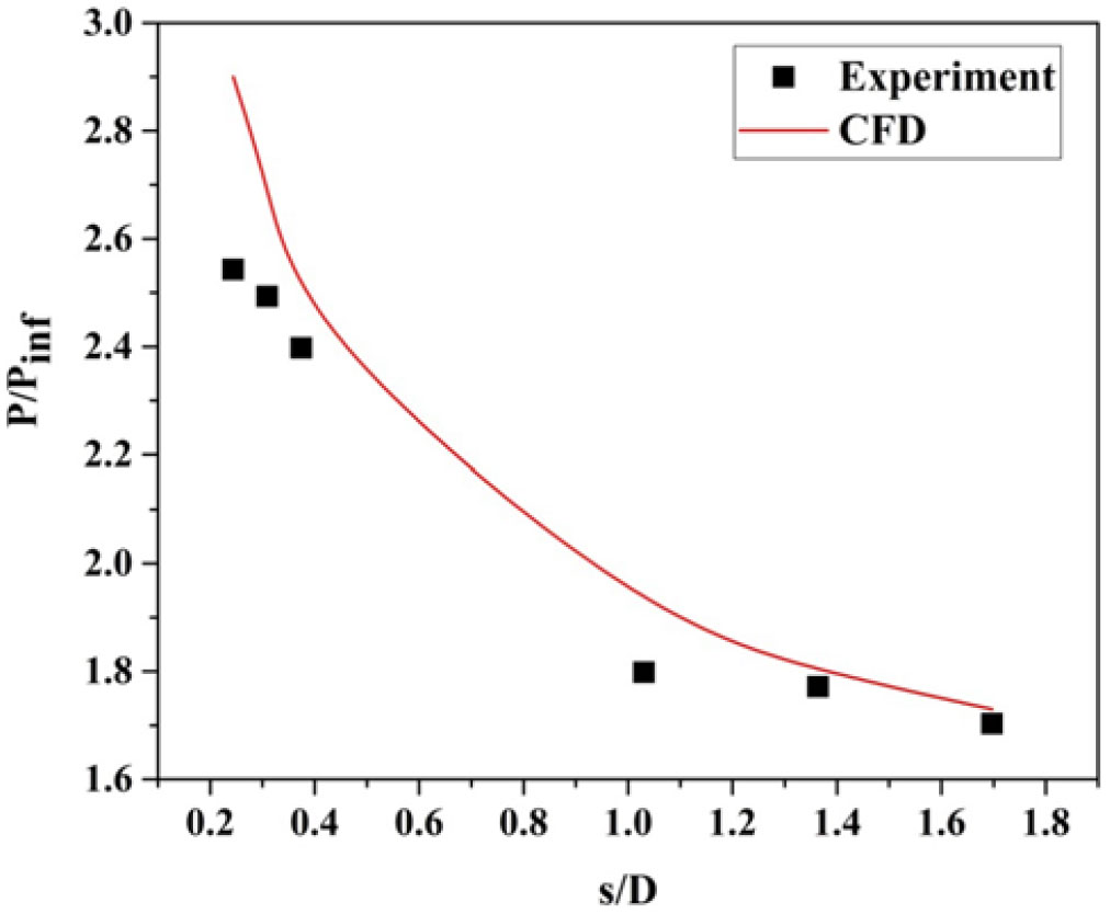
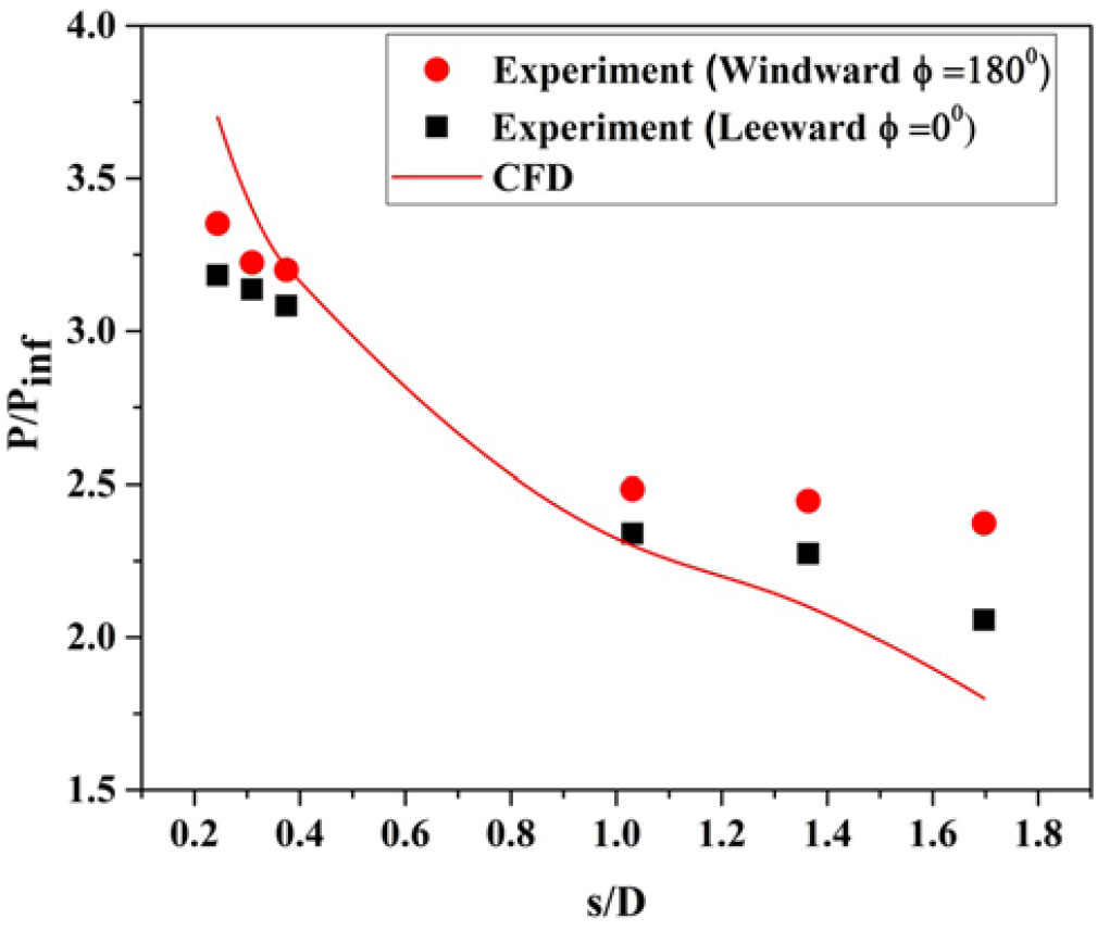
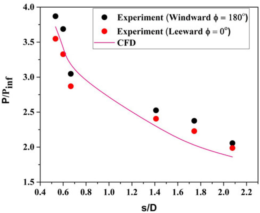
Figure 22. Variation of leeward ( $\phi = 0^{\circ}$) pressure distribution over the surface of a blunt cone model at
  $\alpha = 5^{\circ}$ for M = 6.56.

Figure 23. Variation of windward ( $\phi = 180^{\circ}$) Pressure distribution over the surface of a blunt cone model at
  $\alpha = 5^{\circ}$ for M = 6.56.

Figure 24. Distribution of surface pressure ( $\phi = 90^{\circ}$) over the surface of a blunt cone model at an angle of attack of
  $5^{\circ}$ for M = 6.56.
When the cone model is at an angle of attack, but less than flow deflection angle  $\theta_{\text{c}}$, the streamline at the windward surface (
 $\phi = 180^{\circ}$) crosses the stronger shock wave and acquires a larger entropy. Consequently, the heat transfer rate is higher on the windward surface.The streamline on the leeward surface (
 $\phi = 0^{\circ}$) crosses the weaker shock wave and acquires a weaker entropy and in turn the heat transfer rate is lower compared to the windward surface. All the steamlines along the surface from the windward side are curving upward and also converging in the leeward direction (
 $\phi = 0^{\circ}$).The leeward side has multivalued entropy, ranging from the lowest and the highest within the flow field.
The windward heat transfer rate increases with the angle of incidence, whereas it reduces the heat transfer rate on the leeward surface. The heat transfer rate on windward surface is two to six times higher than on the leeward surface. The heat transfer rate values are substantial in the leading edge (the GS2 and GS3 sensors) but changes in heat transfer rate are moderate along the streamwise length (G1to G6). At  $\alpha = 5^{\circ}$, the percentage of decrease in the windward heat flux at gauge (G6) is 81% of leeward heat and 56% of sideslip heat. According to Fig. 18, the normalized rate of change of heat flux
  $\{q(t)/{Q}_{0}\}$ along the model surface is higher for the windward surface (
 $\phi = 180^{\circ}$) and lower for the leeward surface (
 $\phi = 0^{\circ}$) at
  $\alpha = 5^{\circ}$.
At an angle of attack, as the angle of rotation increases from  $\phi = 0^{\circ}$ at the top surface of the body to
  $\phi = 180^{\circ}$ at the bottom surface of the body, the shock wave shape moves closer to the body surface[Reference Gino and Bleich33] and consequently the heating rate is higher. The heating rate is higher for the windward surface (
 $\phi = 180^{\circ}$) than the sideslip (
 $\phi = 90^{\circ}$) (Fig. 17). The percentage of decrease in the sideslip heating rate (
 $\phi = 90^{\circ}$) and the leeward heating rate (
 $\phi = 0^{\circ}$) along the model length is about 15 to 51%.
There are two significant phenomena that influence the heat transfer. First, the shock wave around a cone model produces an entropy layer that interrelates with the boundary layer that in turn increases the heating rate on the model surface. For axi-symmetric bodies, the flow across the shock wave produces a strong entropy gradient leading to higher vorticity in the direction normal to the velocity at the body surface. These velocity gradients change the boundary-layer velocity profile and in turn generates the heat transfer at the surface of the model surface. The changes in the normal velocity gradient in the direction of the body surface change the boundary-layer shape and consequently transfer heat to the model surface. For 3D bodies, the entropy gradient produces vorticity having a large parallel component to the stream direction outside boundary layer than the normal component and it can affect the heat transfer rate and the boundary-layer stability. Second, viscous interaction between the thick boundary layer of the hypersonic flow and the inviscid flow outside has a significant effect on heat transfer.
The Stanton number is defined as:
 $$C_H = {q\left(t\right)}/{\left\{{\rho }_{inf}V_{inf}\left(H_0-H_w\right)\right\}}$$
where  $q_t$ is the heat transfer rate,
  ${\rho}_{inf}$ is the free-stream density,
  $V_{inf}$ is the free-stream velocity,
  $H_0$ is the stagnation enthalpy, and
  $H_w$ is the wall enthalpy. The variation of the Stanton number along the model surface for two different angles of attack for the blunt cone is shown in Fig. 19. The trend in the variation of heat transfer was preserved for the Stanton variation as well. The Stanton number decreased along the length due to the conical portion of the model. The windward Stanton number is higher than it is for the other cases. The variation in the Stanton number for the windward at
  $\alpha = {0}^\circ$ and the sideslip at
  $\alpha = {5}^\circ$ is not substantial. The windward Stanton number was 2 to 5 times higher than the leeward and 0.9 to 2.2 times higher than the sideslip Stanton numbers.
5.5 Effect of pressure distribution
Heating rate depends not only on the pressure gradient but also on the free-stream density, free-stream temperature, and state of the boundary layer. Like heat transfer, pressure also is measured along the surface of the model for the same angle of attack. The variation of pressure along the surface for the blunt cone and the sharp cone models at  $0^{\circ}$ angle of incidence is shown in Figs. 20 and 21.
At the stagnation point, pressure is high. As flow moves further downstream, the shock strength decreases, thereby the surface pressure decreases along the model surface for sharp cone and blunt cone models. The high pressure that continues to build along the model surface produces a favorable pressure gradient. The pressure gradient is slightly higher on the sharp cone model than on the blunt model.
From Fig. 20, at s/D =0.24 from the nose, the surface pressure distribution predicted by CFD is higher than the experimental value, whereas at s/D = 1.03 the surface pressure measured is higher than that predicted by CFD simulation. For the sharp cone model, as seen from Fig. 21, the surface pressure predicted by CFD is closer to the experimental value. From Fig. 21 a steep drop in the surface pressure near the nose and moderate reduction far away from the nose is observed for the sharp cone model. On the other hand, for the blunt cone model (Fig. 20), the slope of the surface pressure curve is less in the nose as well as in the fa- away region compared to the sharp cone model. This result implies that shock is closer to the surface for the sharp cone model compared to the blunt cone model for the same free-stream condition. Considerable differences can be seen between experimental data and numerical simulation, and the difference may be due to unsteady oscillations in the flow field and the assumption of the turbulent model used in the CFD simulation.
The advantage of the sharp cone model is that the shock wave in the leading edge is attached at the nose, thus the flow behind the sharp cone model does not leak around the leading from bottom to top surface. But in the blunt cone model, the shock wave is detached around the leading edge; hence, there is the possibility of leak in the flow behind the shock around the leading edge. Hence, the higher integrated pressure over the bottom surface is preserved and high lift is generated on the sharp cone model compared to the blunt cone model where relatively lower integrated bottom surface pressure and reduced lift prevail. Therefore, the vehicle having a blunt cone shape must fly at a higher angle of attack to produce the same lift as the sharp cone shape.
The divergence of the measured windward and leeward pressure distibution for both blunt cone and sharp cone models is about 8% at  $\alpha = 0^{\circ}$. The flow field behind the sharp cone model is approximately irrotational
  ${\nabla xV\ =\ 0}$. For the blunt model, the inviscid flow behind the detached shock wave is rotational
  ${\nabla xV \ne 0}$.
High heating rate over the region of windward surface (Fig. 16) is due to the higher pressure gradient (Fig. 23) when compared to the leeward surface where lower heating rate is observed. At  $\alpha = {5}^{\circ}$, about a 36 to 50% decrease in the surface pressure distribution is measured in the windward ray (Fig. 23) and the leeward ray (Fig. 22). About a 2 to 15% decrease in the surface pressure distribution is measured in the windward ray and the sideslip (Fig. 24) at
  $\phi = {90}^{\circ}$ for the same
  $5^{\circ}$ angle of attack.
5.6 Error in heat flux gauges
The error involved in the heat flux sensors can be split as follows:
The uncertainty in the substrate material (MACOR) property:
$\beta = {\sqrt{\rho ck}}$ is $\pm 3.7\%$The uncertainty in the temperature coefficient of resistance:
$\alpha$ is $\pm 2\%$The uncertainty in measuring the initial voltage across the gauge:
$\pm 1.0 \%$The uncertainty in measuring the amplification factor of the signal conditioner is
$\pm 1.0\%: {\rm U}_{\rm q} = \sqrt{3.7^{2} + 2^{2} + 1^{2} + 1^{2}}$The total uncertainty in the measured heat flux (Uq) is 4.43%


6.0 CONCLUSIONS
Heat transfer rate and surface pressure distribution were measured on blunt cone and sharp cone models at a flow Mach number of 6.56. The measured stagnation-point heating rate exceeds the value predicted by the Fay-Riddell correlation and the difference is about 10%. This difference is attributed mainly to the theoretical values of velocity gradient used in the Fay-Riddell correlation. The percentage of increase in heat transfer between the CFD and the experiment is 9%. With an increase in proximity of shock wave to the cone surface, the windward heating rate was higher than the leeward heating rate. At an angle of attack, as angle of rotation increased from  $\phi = 0^{\circ}$ at the top surface of the body to
  $\phi = 180^{\circ}$ at the bottom surface of the body, the shock wave shape moved closer to the body surface and consequently the heating rate was higher. The heating rate was higher for windward (
 $\phi = 180^{\circ}$) than for sideslip (
 $\phi = 90^{\circ}$). The sideslip heating rate was higher than the leeward heating rate (
 $\phi = 0^{\circ}$). This outcome postulated the distribution of convective heating on model surface at an angle of attack demanded the thermal protection system not only at the nose but also at the other parts of model surface. Based on experimental data, the non-dimensional heat flux distribution along the model surface is essentially dependent on body shape and free-stream conditions. The experimentally investigated heat flux distribution and surface pressure distribution along the model surface showed good agreement with the computational result. At
  $\alpha = 5^{\circ}$, the percentage increase in the pressure distribution for the windward and the leeward ray was 36 to 50%. Similarly, for the windward and the sideslip, it was 2 to 15%.
Supplementry Material
To view supplementary material for this article, please visit https://doi.org/10.1017/aer.2019.116