


Introduction
Sub-Antarctica is an oceanic region characterized by the Antarctic Circumpolar Current, flowing from west to east around the Antarctic continent and which is mainly driven by the westerly winds. Several ocean fronts occur, of which the Polar Frontal Zone (PFZ), where cold northward-flowing Antarctic water masses confront and sink beneath warmer sub-Antarctic water masses, is the most important one. In this specific oceanic region, only six islands or archipelagos occur, scattered around the PFZ. Sub-Antarctic islands are characterized by treeless vegetation, and those lying south or on the PFZ are partially glaciated. Others are ice-free today but show evidence of a more widespread glaciation in the past. Thus, glaciation and postglacial deglaciation events such as glacier retreat and advance and isostatic movements have been powerful shapers of sub-Antarctic landforms. However, other geomorphological processes, such as tectonics, are also important in moulding sub-Antarctic landscapes (Selkirk et al. Reference Selkirk, Adamson and Wilson1990, Adamson et al. Reference Adamson, Selkirk, Price, Ward and Selkirk1996).
Previous studies (Clapperton Reference Clapperton1971, Clapperton et al. Reference Clapperton, Sugden, Birnie and Wilson1989) of landforms and the geomorphological and environmental evolution of South Georgia since the Last Glacial Maximum (LGM) are based on mapping of glacial features together with evidence from slope stratigraphy and peat and lake records. The chronology of the glacial history in these studies is based on radiocarbon dating of basal peat and intercalated peat beds in slope exposures. The area investigated here covers mainly Cumberland and Stromness bays, readily accessible areas around the former whaling stations Grytviken and Husvik, but also the Possession and Antarctic bays (Fig. 1). In a recent study, Bentley et al. (Reference Bentley, Evans, Fogwill, Hansom, Sugden and Kubik2007a) revisited those areas and mapped in detail former glacier margins together with other geomorphological features. Cosmogenic 10Be nuclide ages of boulders constrained the ages of the moraines.

Fig. 1 South Georgia showing the location of the study area. The inset shows an overview of the Sromness Bay/Husvik area with locations of the existing radiocarbon dates, 10Be exposure ages and the Last Glacial Maximum (LGM) limit of the fjord glacier. Unofficial names, used in the text, are written in italics on the map.
Both the extent of the LGM ice cover as well as the timing of deglaciation of the lower parts of the island is still a matter of debate. Clapperton et al. (Reference Clapperton, Sugden, Birnie and Wilson1989) suggested an ice cap maximum extent to the edge of the continental shelf at least 18 000 14C years ago followed by a wastage of this ice cap with two periods of glacier re-advance (somewhere between 18 000 and 14 000 14C yr bp and > 9700 14C yr bp) but these advances are not chronologically well constrained. Raised beach deposits associated with both periods of glacier re-advance have been described by Clapperton et al. (Reference Clapperton, Sugden, Birnie and Wilson1989). A first set is found at an altitude of 6–10 m a.s.l. and was formed after retreat of the oldest glacier re-advance (14 000–18 000 14C yr bp), and a second set occurs at an altitude of 2–3 m a.s.l. and is connected to the glacier re-advance >9700 14C yr bp (Clapperton et al. Reference Clapperton, Sugden, Birnie and Wilson1989). Bentley et al. (Reference Bentley, Evans, Fogwill, Hansom, Sugden and Kubik2007a) provided 10Be nuclide ages for a number of moraines and suggested a LGM ice extent which was restricted to the inner fjords (Fig. 1). Gravel beach ridges and marine terraces have been mapped by these authors up to an altitude of c. 7 m. Graham et al. (Reference Graham, Fretwell, Larter, Hodgson, Wilson, Tate and Morris2008), based on a compilation of marine echo-sounding datasets, allowing mapping of the geomorphology of the continental shelf of South Georgia, concluded that ice sheets extended to the shelf break at least once (but probably numerous times). Although the authors stated that the age of the shelf morphology may date back to late Miocene times, they left the possibility open that extensive glaciation occurred also at the LGM.
There is a consensus that the lower parts of the island were ice-free in the early Holocene based on radiocarbon dating of basal peat deposits (Van der Putten & Verbruggen Reference Van der Putten and Verbruggen2005 and references therein). The timing of deglaciation is, however, still debated. Based on a unique lake record, Rosqvist et al. (Reference Rosqvist, Rietti-Shati and Shemesh1999) proposed that deglaciation commenced prior to 18 600 cal yr bp. Radiocarbon dating of basal peat deposits as well as 10Be nuclide ages of moraines in inner Husvik fjord, suggest, however, that ice was still present in the inner fjord for a much longer time span (Fig. 1, for further discussion we refer to Van der Putten & Verbruggen Reference Van der Putten and Verbruggen2005, Reference Van der Putten and Verbruggen2007 and Bentley et al. Reference Bentley, Evans, Fogwill, Hansom, Sugden and Kubik2007b).
This study aims to reconstruct the geomorphology and Holocene landscape evolution of the inner fjord of Husvik Harbour, Stromness Bay, also called Husdal (unofficial name) based on the lithostratigraphy of the area by means of corings, together with diatom analysis of the different sedimentological units and radiocarbon dating. The methodology used adds information on the area for which detailed surface geomorphological maps are available. One of the features mapped in the ‘Husdal’ area by Clapperton (Reference Clapperton1971) and Bentley et al. (Reference Bentley, Evans, Fogwill, Hansom, Sugden and Kubik2007a) are raised beaches/gravel beach ridges. The extent and thickness of ice cover in combination with the deglaciation chronology have influenced the isostatic depression and subsequent rebound of the island and hence the presence and altitude of raised beaches. Although we present no direct evidence on the LGM ice extent, this study can contribute to the larger discussion of the glaciation and deglaciation history of South Georgia. Moreover, our results contribute to the knowledge of where continuous and complete Holocene peat sequences for palaeoenvironmental research can be found in the Husvik Harbour area.
Study area
The island of South Georgia (c. 170 km long and 2–34 km wide) is situated in the South Atlantic Ocean (54°30′–55°00′S; 35°30′–38°30′W), c. 1300 km ESE of the Falkland Islands (Fig. 1). The elongated Allardyce mountain range extends WNW–ESE, culminating in Mount Paget at 2934 m (Fig. 1). The northern coast is indented by deep fjords.
The climate of South Georgia is cold, wet and cloudy with strong winds, subject to rapid changes without great seasonal variation and a mean annual temperature of +2.0°C (Headland Reference Headland1984). August is the coldest month with a mean temperature of -1.2°C, whereas February is the warmest with +5.6°C. The mean annual precipitation at King Edward Point, Grytviken (Fig. 1) is 1602 mm (Headland Reference Headland1984). Permanent ice and glaciers, descending to sea level, cover 58% of the surface (Clapperton Reference Clapperton1971). South Georgia is situated south of the Polar Front and thus has a harsher climate than some other islands included in the sub-Antarctic Botanical Zone by Greene (Reference Greene1964). Ice-free parts of the island are covered with tundra-like vegetation, lacking arborescent vascular plants. The climatic conditions are suitable for peat formation and extensive peat cover has developed at lower altitudes, with thicknesses between 1 and 5 m.
‘Husdal’, defined in this study as the area covering the lower part of Husvik Harbour (see dashed box in Fig. 1), is situated on the north coast of the island and forms the southern part of the larger Stromness Bay (Fig. 1). The bay is divided into two smaller fjords by the Tønsberg peninsula (unofficial name). In each fjord there is an ancient whaling station, Husvik and Stromness. Both station sites make use of the river flats that are formed at the inner side of the fjords. The area of ‘Husdal’ occupies c. 1 km2 and is drained by two rivers: the Husvik river (unofficial name) in the north and the Husdal river (unofficial name) in the south. The catchment area of both rivers is c. 15 km2. The geomorphological map of Clapperton (Reference Clapperton1971) shows the presence of till, moraine ridges, roches moutonnées, fluvio-glacial deposits and raised beaches. Bentley et al. (Reference Bentley, Evans, Fogwill, Hansom, Sugden and Kubik2007a) mapped the area in more detail showing lateral moraines, kame terraces, gravel beach ridges and the braided outwash of both rivers. Some of the features described by Clapperton (Reference Clapperton1971) were re-interpreted by Bentley et al. (Reference Bentley, Evans, Fogwill, Hansom, Sugden and Kubik2007a).
The geomorphological setting
The landscape at the fjord head in Husvik Harbour contains features formed by glacial, alluvial and littoral processes.
A 10–25 m wide beach forms the present-day coastline. Landward of the active beach (up to c. 100 m inland) is a set of older beaches with spits and (palaeo)lagoons. The present-day beach blocks the outflow of the Husdal and Husvik rivers, and close to the coast the rivers flow parallel with the beach some distance before cutting through.
Behind this beach system a rather flat plain extends inland. The plain partly consists of the active braided river outwash from the Husdal and Husvik rivers, and partly of peat-covered areas. In the central part of the vegetated area a few elongated features occur. They are slightly elevated above the plain and are oriented more or less parallel to the coast. A bedrock outcrop is visible in one of the ridges. The most landward of the elongated features (at core site 2 in Fig. 2) differs from the others as it is broader and has steep, fairly high edges (estimated up to 3 m). These landforms were interpreted as raised beaches by Clapperton (Reference Clapperton1971) and as beach ridges (the outer ones) and kame terraces (the inner one) by Bentley et al. (Reference Bentley, Evans, Fogwill, Hansom, Sugden and Kubik2007a, see fig. 10d, p. 662).

Fig. 2 Geomorphological map and cross-section of ‘Husdal’.
The sharp eastward edge of the inner ridge forms a prominent linear feature in the landscape and can be followed discontinuously both to the north and the south (line M in Figs 1 & 2). To the north, the scarp gradually disappears under the outwash of the Husvik river and in the south it partly merges with the seaward limits of bedrock outcrops.
The bedrock outcrops are glacially eroded and some of them form roches moutonnées. The outcrops belong to a bedrock threshold stretching across the Husdal river valley, and they force the braided Husdal river through a narrow gap while both up- and downstream of the threshold (∼ line M), the outwash is able to spread over wider areas. Further upstream the Husdal river flows through a canyon, at the mouth of which the alluvial fan has its apex. Upstream of the canyon, the Husdal river builds up another alluvial fan, at an elevation of about 150 m a.s.l. The Husvik river to the north also forms a braided river system and the Husvik whaling station is built on its alluvial fan.
Outside the active alluvial fans are fossil alluvial deposits, glacial features (roches moutonnées, moraines) and bedrock with no or little sediment cover. The fossil alluvium is vegetated and some of the areas are bounded by erosional scarps. The glacial deposits and landforms have been mapped by both Clapperton (Reference Clapperton1971) and Bentley et al. (Reference Bentley, Evans, Fogwill, Hansom, Sugden and Kubik2007a) and more details can be found on their maps. Among the recognized landforms are several lateral moraines on the valley sides (Bentley et al. Reference Bentley, Evans, Fogwill, Hansom, Sugden and Kubik2007a) where otherwise the bedrock is exposed or covered by scree.
Methods
Map information
Besides the published geomorphological maps (Clapperton Reference Clapperton1971, Bentley et al. Reference Bentley, Evans, Fogwill, Hansom, Sugden and Kubik2007a) we made use of the chart of the Stromness Bay area and of a stereo-pair of aerial photographs of ‘Husdal’, made available by the Operational Support Flight, Joint Air Reconnaissance Intelligence Centre (JARIC), RAF Brampton, Huntingdon, UK. The latter were very useful, allowing us to recognize and draw the approximate borders of the geomorphological features important for this study. The chart reveals an obvious change to deeper water seaward of the line between Kanin Point and Brain Island (Fig. 2). At the same place the aerial photograph shows a constriction of the coastline and a row of emerging rocks, underlining the presence of a distinct bedrock threshold in the Husvik fjord.
By means of vertical photogrammetric measurements a topographical profile was drawn approximately along a line of three of the core sites (1b, 2 and 3b) in order to construct the cross-section presented in Fig. 2. No exact altitudes a.s.l. could be determined in the field. However, the stereo-pair of aerial photographs allowed us to define approximate altitudes and especially allowed us to distinguish the relative height of the different landforms in relation to each other.
Field survey
In the summer of 1992–93 and 1995–96 fieldwork was conducted in the inner fjord of Husvik Harbour and the Tønsberg peninsula. The initial focus of the fieldwork was to survey the peat cover to detect deep peat sequences for palaeobotanical research (Van der Putten et al. Reference Van der Putten, Mauquoy, Verbruggen and Björck2004, Reference Van der Putten, Stieperaere, Verbruggen and Ochyra2009, Reference Van der Putten, Verbruggen, Ochyra, Spassov, De Beaulieu, De Dapper, Hus and Thouveny2012). Based on the geomorphology of the area, the thicknesses as well as the character of the peat deposits, and the lithology of the underlying sediments, six sites were chosen for deep coring (Fig. 2). The peat cover was surveyed by manual coring with augers and a gouge. For deep coring we used a water pump, together with casings, to flush up the sediments. This flush-coring method allowed us to penetrate sand and gravel layers as well as intercalated peat layers where present, and to investigate the sediment stratigraphy of the subsoil of the ‘Husdal’ plain. The disadvantage of this method is that we could only recover disturbed “flushed up” sediments and did not obtain preservation of the sedimentary structures as would have been the case with a core. However, using casings makes it possible to keep the borehole open and at any time flushing could be stopped and sediments/peat could be retrieved with hand coring equipment. In this way, the different sedimentological units were sampled for diatom analysis and peat was recovered for radiocarbon dating. Where possible the maximum-equipment-depth of 11 m was obtained. In one case the bedrock was reached (core 3a) and one coring had to be stopped as the sediment texture and/or the hydrological conditions impeded further penetration (core 2). Coring 1c was stopped deliberately at 7 m since the general stratigraphy was identical to the stratigraphy in cores 1a and 1b.
Radiocarbon dating
Four bulk samples of basal peat and intercalated peat deposits were submitted for 14C dating shortly after the field campaign. A fifth date was obtained from fossil phaeophyte remains (seaweed) found in a sand layer (core 1a) and a sixth one from a recent phaeophyte in order to identify the reservoir effect of seawater around South Georgia.
For the Antarctic, a general pre-bomb marine reservoir correction of 1300 years has been proposed (Berkman et al. Reference Berkman, Andrews, Björck, Colhoun, Emslie, Goodwin, Hall, Hart, Hirakawa, Igarashi, Ingólfsson, Lopez-Martinéz, Lyons, Mabin, Quilty, Taviani and Yoshida1998). As the recent sample of phaeophyte was collected in 1995 we are dealing with a post-bomb sample resulting in a possibly younger measured 14C age. For this reason, we decided to use both data as the extreme limits for the determination of the reservoir correction of the 14C date of the fossil phaeophyte.
Samples were pre-treated by the routine AAA (acid alkali acid) method and AMS targets prepared by routine methods (Van Strydonck & Van den Borg Reference Van Strydonck and van den Borg1991) at the Royal Institute for Cultural Heritage (Brussels, Belgium). Samples were measured at the Van de Graaff laboratory (Utrecht, The Netherlands). Calibration of radiocarbon dates was performed using the Calib ver. 6.0.1 program (Reimer et al. Reference Reimer, Baillie and Bard2004) and the Southern Hemisphere calibration dataset (McCormac et al. Reference McCormac, Hogg, Blackwell, Buck, Higham and Reimer2004). All ages in the paper are calibrated (except when stated otherwise) and are reported as the central point estimates determined by the median of the probability distribution.
Diatom analysis
Samples at eleven levels of cores 1a, 1b, 1c and 3b have been analysed for their diatom content. Samples were prepared following the method described in Van der Werff (Reference Van der Werff1955). In some samples the preservation of the frustules was poor and/or the number of species restricted. However, the analysis produced sufficient information to classify the sediments as deposited in a marine or a freshwater environment. These data are included in the sediment logs of Fig. 3.

Fig. 3 Sediment logs of the six cores sites. The marked depths of the transitions between the different units in the environment/morphogenesis log are taken from the coring situated the closest to the cross-section.
Results and analyses
Sediments and stratigraphy
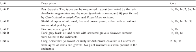
Five sedimentological units could be distinguished based on lithological properties. The units are named in stratigraphic order from A (lowest) to E (uppermost) and are described in Table I and their stratigraphic relationship is shown in the logs in Fig. 3.
Table I Description of the sedimentological units. The units are named in stratigraphic order from A (lowest) to E (uppermost). The core numbers refer to the logs in Fig. 3.
Diatom analysis
Core 1a
Two samples from Unit B (550 cm and 900 cm depth) were analysed. The diatom flora in these samples clearly reflects marine conditions. A well developed marine flora was found containing a large number of species of which Gomphonemopsis littoralis (Hendey) Medlin and Navicula aff. perminuta Grunow are the most dominant ones. Valves belonging to Licmophora sp., Haslea sp. and several Cocconeis species were likewise found.
Core 1b
Four samples from Unit B (450, 600, 700 and 1050 cm depth) and one sample from Unit D (220 cm) were analysed. The sample at 220 cm depth is clearly a freshwater sample reflecting a well developed diatom flora containing Planothidium lanceolatum (Bréb.) Lange-Bertalot as the most dominant species. Other important species include Psammothidium subatomoides (Hust.) Bukh. & Round, Gomphonema parvulum (Kütz.) Kütz., Staurosira subsalina (Hust.) and Fragilaria capucina Desmazières.
At a depth of 450 cm, only marine valves were present. Several species of Cocconeis (such as C. imperatrix A. Schmidt, C. scutellum Ehrenb. and C. costata Gregory) were found. Freshwater or terrestrial valves were absent. The amount of unbroken valves found in the sample is rather low.
The samples at 600, 700 and 1050 cm contain eroded fragments of marine diatom species, including Thalassiosira sp., Cocconeis sp. and Thalassionema. The low quality of the remains did not allow a complete identification up to the species level.
Core 1c
A sample from Unit B at 430 cm depth shows a similar marine flora as the one found in core 1a but there is a dominance of the larger Cocconeis valves belonging to species such as Cocconeis imperatrix and C. costata.
Core 3b
Samples were taken from Unit A (1100 cm depth) and from Unit D (at depths of 180, 240, 320 cm). Although the number of diatoms found in the sample at 180 cm depth is rather low compared with the sample at 220 cm in core 1b, the floras are strikingly similar, reflecting a freshwater diatom flora. In the other samples of core 3b only a restricted number of fragments of freshwater species were found. Due to the poor quality of the remains, it was hardly possible to identify them up to the species level.
Radiocarbon dating
This study is based on the results of five new 14C dates (Table II) on organic material from different levels in the cores of ‘Husdal’ area (Fig. 3). A sixth dating of a recent phaeophyte (Utc-6873, 465 ± 30 14C yr bp) was made to identify the reservoir effect of seawater around South Georgia (Table II).
Table II Radiocarbon dates for the ‘Husdal’ area. All samples are bulk peat samples except for: *fossil phaeophyte remains, and ‡recent phaeophyte remains in order to identify the reservoir effect. The central point estimate was determined by the median of the probability distribution.
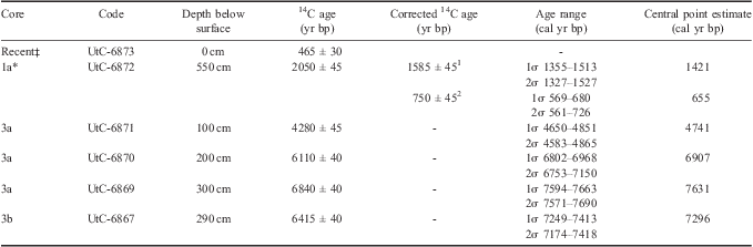
1marine reservoir correction of 465 years.
2marine reservoir correction of 1300 years.
Interpretation of the sediments and the diatom data
Unit A: glaciofluvial deposits
The variable grain size with occasional coarser layers together with the absence of plant remains suggest that Unit A can be interpreted as a glaciofluvial deposit, which is supported by the stratification (Fig. 3). The low numbers of fragmented freshwater diatom valves in the samples beneath 540 cm in core 3b support this interpretation.
Unit B: shallow marine silt and sand deposits
Dark grey-black silt and sands with scattered gravels were found to a depth of 11 m. The grain size, particularly the abundance of sand, indicates that the water probably was fairly shallow. The diatom species found clearly suggest that the sediments were deposited in a marine environment which is also supported by the presence of seaweed remains.
The ecology of a large number of the encountered valves in core 1a points to the presence of a macro-algal community (Witkowski et al. Reference Witkowski, Lange-Bertalot and Metzeltin2000). For instance, G. littoralis, Licmophora sp., Haslea sp. and several Cocconeis species are known to prefer a typical epiphytic life-form. On the other hand, typical planktonic species such as Thalassiosira sp. are almost entirely absent.
The presence in core 1b (450 cm) of several species of Cocconeis (such as C. imperatrix, C. scutellum and C. costata), which usually attach to the substrate and/or macro-algae in the subtidal zone, clearly indicates a marine environment (Riaux-Gobin & Romero Reference Riaux-Gobin and Romero2003). The samples at 600, 700 and 1050 cm contain eroded fragments of marine diatom species, including Thalassiosira sp., Cocconeis sp. and Thalassionema. The low quality of the remains did not allow a complete identification up to the species level. Nevertheless it is clear that this was a purely marine environment. The reason for the bad preservation of diatom valves is unclear, but it could be the result of a highly turbulent environment.
The dominance of the larger Cocconeis valves belonging to species such as C. imperatrix and C. costata in the sample at 430 cm depth from core 1c probably reflects more littoral conditions without a large macro-algal presence.
Unit C: beach gravel deposits
This unit consists of well-sorted fine and coarse gravel and is interpreted as being formed at a beach, similar to the one close to the present coastline.
Unit D: alluvial deposits
The stratified layers of silt, sand, fine and coarse gravel together with, in some cases, the presence of intercalated peat layers suggests that Unit D deposits are most probably formed in an alluvial environment. An alternative possibility is that the mixed clastic sediment and peat layers may represent tsunami deposits (e.g. Grauert et al. Reference Grauert, Björck and Bondevik2001). However, the diatom flora of the samples in cores 1b (220 cm) and 3b (180, 240 and 320 cm) are clearly characteristic of a freshwater environment. The dominant species in core 1b, P. lanceolatum, is widely distributed on South Georgia and the other sub-Antarctic islands and is usually typical of running water conditions (Van de Vijver & Beyens Reference Van de Vijver and Beyens1996, Van de Vijver et al. Reference Van de Vijver, Frenot and Beyens2002). Only one marine valve was found in this sample: C. imperatrix, most probably the result of wind activity.
In core 3b at 180 cm depth, only freshwater species were found including Pinnularia viridiformis Krammer and Staurosira pinnata Ehrenberg which are typical of larger open freshwater lakes and pools (Van de Vijver et al. Reference Van de Vijver, Frenot and Beyens2002).
The frequent changes in the texture of the sediments points to quickly changing conditions in the river plain, due to a dynamic braided river system. Peat could develop on the river plains during short periods when the river channels were active on other parts of the fan, and fluvial activity was abandoned at the core site. The abundance and preservation of the diatom valves is poor but only freshwater species were found.
Unit E: mire and moss peat
The two types of peat represent different hydrological conditions. The peat dominated by the rush Rostkovia magellanica (Lamark) Hooker and the moss Syntrichia robusta (Hook. & Grev.) is a mire peat, pointing to wetter and more eutrophic conditions in a river plain. The peat formed by Chorisodontium aciphyllum (Hook. f. & Wilson) and Polytrichum strictum Menz. ex. Brid. is a moss peat and reflects dryer and more oligotrophic conditions.
Postglacial landscape evolution of ‘Husdal’
Unit B is found in the bottom of cores 1a, 1b and 1c (Fig. 3), and extends seaward of line M (c. 9 m a.s.l.), suggesting a marine infilling at the fjord head (Fig. 2). The sediment sequence shows a development from a relatively deep bay (> 7 m) filling the accommodation space with sediments (Unit B), until the shallowing ends up in coarse gravels representing a beach (Unit C). Layers of varying grain size with freshwater diatom species (fluvial deposits up to > 3 m thickness) were found on top of Unit C forming an alluvial plain (Unit D).
Landward of line M no marine sediments were found (cf. cores 2, 3a and 3b), thus line M is the most probable inland position of any former coastline in the Husvik fjord. One possibility is that line M is a wave-cut erosional form representing the highest coastline and that the plain seaward of line M was built up by gravel beach ridges due to isostatic rebound as proposed by both Clapperton (Reference Clapperton1971) and Bentley et al. (Reference Bentley, Evans, Fogwill, Hansom, Sugden and Kubik2007a). However, the freshwater origin (based on the diatom analysis in core 1b) of the uppermost three metres of alluvial sediments contradicts the presence of beaches. Another possibility is that the sharp edge of line M is not formed by marine erosion but by alluvial erosion by the Husdal river and/or Husvik river at times when they followed a different course.
Landward of line M, a more elevated zone occurs (Fig. 2). Roches moutonnées are incorporated in this zone suggesting a bedrock threshold below or just inland of line M. A similar sill is present in the Husvik fjord, below sea level, along the line between Kanin Point and Brain Island. Core 2 shows that beneath a peat layer of > 1 m thickness glaciofluvial sediments are present (Unit A, Fig. 3). Those sediments possibly correspond to the mapped kame deposits of Bentley et al. (Reference Bentley, Evans, Fogwill, Hansom, Sugden and Kubik2007a). A temporary standstill of the retreating glacier or a rapid downwasting of ice at the bedrock obstacle can explain the extensive deposition of glaciofluvial sediments. These deposits were later eroded by rivers and now form erosional remnants in the landscape. With such an interpretation we cannot determine the altitude of the highest relative sea level, but we know that line M is the most inland position of the coastline since the deglaciation of the area, based on the presence of marine sediments. However, from our data it is not possible to interpret the elevated area (c. 12 m a.s.l.) landward of line M as a raised beach deposit as suggested by Clapperton (Reference Clapperton1971).
Landward of the more elevated zone, outside the active outwash plains of the Husvik and Husdal rivers, a lower lying area occurs, which has been filled in by alluvial deposits of the Husdal river and maybe also by the Husvik river, with a minimum thickness of 3 m (Unit D, cores 3a and 3b, Figs 2 & 3). A relatively thin peat layer (0.2 m up to 2 m) is found on top of the alluvial deposits, as well as intercalated peat layers in between the gravel and sand deposits. These “fossil” alluvial deposits cover the glaciofluvial sediments of Unit A. As mentioned, the former coastline (line M) cannot be distinguished in the northern part of the study area due to the large and stony alluvial fan of the Husvik river and/or the lower altitude of the scarp. There is a marked difference between the coarse gravels and sands of the northern Husvik river and the relatively fine textured sediments with intercalated peat bands in the southern Husdal river plain. This can be explained by the fact that the Husdal river has a second broad alluvial flat upstream, at an elevation of about 150 m where the coarser sediments have been captured.
Discussion
Regarding the relation between sea level and deglaciation we have two key questions: when was the area deglaciated, and how much of the isostatic uplift remained at deglaciation?
The glaciofluvial Unit A was deposited during the deglaciation of ‘Husdal’, which was completed in the early Holocene (Smith Reference Smith1981, Clapperton et al. Reference Clapperton, Sugden, Birnie and Wilson1989, Van der Putten & Verbruggen Reference Van der Putten and Verbruggen2005). Previous studies (Van der Putten & Verbruggen Reference Van der Putten and Verbruggen2005 and references therein) have presented many radiocarbon dates for the area around Husvik Harbour outside the alluvial plain. These dates have been carried out on lake sediments and on the base of peat deposits. The oldest radiocarbon date of basal peat in the area is sampled at a depth of 460 cm in a peat sequence south and uphill of the active outwash plain of the Husdal river and gives an age of c. 10 300 cal yr bp (Van der Putten et al. Reference Van der Putten, Mauquoy, Verbruggen and Björck2012), which is a minimum age of the deglaciation. Other basal peat dates of early Holocene age (10 700 and 9100 cal yr bp respectively) are found on the eastern part of the Tønsberg peninsula and at Kanin Point (Fig. 1; Van der Putten et al. Reference Van der Putten, Stieperaere, Verbruggen and Ochyra2004, Reference Van der Putten, Verbruggen, Ochyra, Spassov, De Beaulieu, De Dapper, Hus and Thouveny2009). Lake sediments (Rosqvist et al. Reference Rosqvist, Rietti-Shati and Shemesh1999) and exposure datings (Bentley et al. Reference Bentley, Evans, Fogwill, Hansom, Sugden and Kubik2007a) give ages between 18 000 and 12 000 cal yr bp respectively (Fig. 1). Exposure datings are more prone to dating errors, up to 1800 years (Bentley et al. Reference Bentley, Evans, Fogwill, Hansom, Sugden and Kubik2007a). However, the exposure dates of c. 12 000 cal yr bp are in agreement with an early Holocene withdrawal of the ice from the fjord head.
Isostatic uplift as a consequence of deglaciation of a formerly glaciated area is a normal feature, and the balance between remaining uplift and sea level rise in coastal deglaciated areas will determine the possibility of forming raised beaches. A large ice cap (ice load) will give rise to more isostatic depression and thus more uplift and raised beaches at higher elevations than a restricted ice cap. In our case of Stromness Bay, it might be possible to use our new results to distinguish between the extensive ice cap of Clapperton and the restricted ice of Bentley et al. (Reference Bentley, Evans, Fogwill, Hansom, Sugden and Kubik2007a).
Assuming that ‘Husdal’ was finally deglaciated as late as in the early Holocene (see above), the deglaciation would take place at a time when the eustatic sea level was still 40–60 m lower than today (Fleming et al. Reference Fleming, Johnston, Zwartz, Yokoyama, Lambeck and Chappell1998, Siddall et al. Reference Siddall, Rohling, Almogi-Labin, Hemleben, Meischner, Schmelzer and Smeed2003). With a restricted LGM ice extent (Bentley et al. Reference Bentley, Evans, Fogwill, Hansom, Sugden and Kubik2007a), and thus a rather restricted isostatic depression, the isostatic rebound would almost have ceased by the early Holocene. With such prerequisites, relative sea level in the Husvik fjord during the early Holocene was most probably lower than today. We would then expect terrestrial (glaciofluvial/alluvial) sediments to be transported and deposited beyond the present coastline. Assuming no or very little remaining isostatic uplift, the Holocene eustatic sea level rise would result in a transgression in the bay. Such a change of base level would cause a decrease in river gradients, and allow deposition rather than erosion to dominate the (presently) lower reaches of the Husdal and Husvik rivers. If the LGM ice extent was more extensive (Clapperton et al. Reference Clapperton, Sugden, Birnie and Wilson1989), and the isostatic depression thereby larger, we would expect that some uplift would have remained by the early Holocene, that relative sea level at deglaciation was higher and that raised beaches would have formed at a higher elevation than in the case of a restricted ice sheet. Whereas we have no sedimentary evidence from offshore to reject or support a lower sea level in the early Holocene, the start of postglacial infilling (Unit D) of the Husdal river plain upstream of the outlet through line M may well reflect a rise in base (sea) level. The infilling started soon after 8000 cal yr bp (based on the basal peat dates in the cores 3a and 3b), which suggests that prior to this time, this part of the river system was mainly erosional and the alluvial deposits were transported and deposited beyond the present coastline, as proposed above. Alternatively, the Husdal river functioned as a glaciofluvial drainage system, depositing Unit A until a few thousand years after deglaciation of the coast. The former would imply higher energy levels and possibly also high sedimentation rates at and outside the mouth of the river, in the marine bay below today's sea level.
The presence of marine sediments east of line M (Fig. 2) shows that the sea once reached that far inland, but sea level does not need to have been much higher than today (see above). It is not possible to date when line M became the coastline, if it ever did. However, global sea level changes show that the decay of the large ice sheets was completed 6000 years ago and that since that time only minor fluctuations have occurred (Fleming et al.Reference Fleming, Johnston, Zwartz, Yokoyama, Lambeck and Chappell1998, Siddall et al. Reference Siddall, Rohling, Almogi-Labin, Hemleben, Meischner, Schmelzer and Smeed2003) suggesting that it happened in the early to mid-Holocene.
Our results partly contradict the interpretation of two sets of raised beaches by Clapperton (Reference Clapperton1971) in this area. He recognized an upper raised beach (6–10 m a.s.l. and post-dating the oldest glacier re-advance at 14 000–18 000 14C yr bp) and a lower raised beach (2–3 m a.s.l. and assumed to be from an early Holocene age connected to the glacier re-advance >9700 14C yr bp). Considering the geomorphological map in Clapperton (Reference Clapperton1971) the lower raised beach is the area situated seaward of line M (see also Fig. 4) where three metres of alluvial freshwater sediments were found (Unit D), whereas the upper one corresponds to the more elevated zone (core 2 and Fig. 3), which we show to consist of glaciofluvial deposits (Unit A). Therefore we cannot agree with the interpretation of the two sets of raised beaches. Although we could not precisely determine the elevation of the buried beach gravel in cores 1a and 1b, it is approximately situated at today's sea level. Since a beach is normally formed at a higher elevation than mean sea level it would imply that the area was slightly transgressed during the formation of Unit C, the beach gravel. The transition from marine sediments to alluvial sediments seaward of line M took place later than 1420/650 cal yr bp based on the two possible reservoir ages (Table II). Since that time the alluvial plain has expanded seaward of line M, and taking into consideration the thickness of the alluvial sediments (up to 3.20 m), this new river plain has been the main area of deposition in the last few hundred years. This suggests a reasonably stable sea level that allows aggradation and progradation due to sediment infill, rather than coastline progradation due to land uplift.

Fig. 4 Overview of the seaward part of ‘Husdal’ with a view on the Tønsberg peninsula and the location of core site 1a. In the background (left upper corner) Husvik whaling station can be seen. The picture has been taken on top of one of the roches moutonnées (Fig. 1).
We conclude that the remaining isostatic uplift during deglaciation was smaller than the difference between the early Holocene and current sea level. This suggests that during the Holocene, the rise of sea level was faster than, or more or less kept in pace with the isostatic rebound at least on this part of the island. In consequence, our data correspond to a rather restricted LGM ice extent as suggested by Bentley et al. (Reference Bentley, Evans, Fogwill, Hansom, Sugden and Kubik2007a).
The onset of peat formation (Unit E) in the Husvik Harbour area is likewise controlled by the postglacial landscape evolution. The youngest peat deposits (< 1000 years) are found seaward of line M. Landward of line M, in the “fossil” alluvial plain area, older peat deposits (< 8000 years) occur, intercalated with alluvial sediments. However, continuous and complete peat sequences suitable for palaeoenvironmental research should be sampled outside the active and “fossil” alluvial plains, for example: i) in glacially eroded rock depressions (Tønsberg peninsula; Van der Putten et al. Reference Van der Putten, Stieperaere, Verbruggen and Ochyra2004), ii) on top of glacial sediments where moss peat banks, dominated by the moss species C. aciphyllum and P. strictum, occur (Kanin Point; Van der Putten et al. Reference Van der Putten, Verbruggen, Ochyra, Spassov, De Beaulieu, De Dapper, Hus and Thouveny2009), and iii) on gentle valley slopes where mire peat develops (Van der Putten et al. Reference Van der Putten, Mauquoy, Verbruggen and Björck2012).
Summary and conclusion
Glaciofluvial sediments (Unit A) were deposited during deglaciation prior to 10 300 cal yr bp. Between 10 300 and 8000 cal yr bp, no alluvial sediments were deposited in the “fossil” alluvial plain area landward of line M. Accepting that ‘Husdal’ was ice-free at least by 10 300 cal yr bp, we consider this period as an erosional/transportational phase with deposition of alluvial sediments beyond the present coastline because sea level was considerably lower in the early Holocene. The position of and relationship between marine Unit B, littoral Unit C and alluvial Unit D reflect postglacial sea level changes and related modifications of river gradients. By c. 8000 cal yr bp, sea level had raised high enough to allow alluvial sedimentation and peat growth landward of line M due to a decrease in the river gradients. Seaward of line M, sedimentation in a marine environment occurred, resulting in the deposition of Unit B. Roughly 1000 years ago the shallowing of the bay culminated in the deposition of coarse beach gravel (Unit C) followed by the expansion of the alluvial plain of both rivers (Unit D) seaward of line M. The postglacial geomorphological evolution of ‘Husdal’ was controlled by fluvio-deltaic deposition as a result of a postglacial sea level rise that was faster than, or kept in pace with the isostatic rebound of the land.
Acknowledgements
British Antarctic Survey, Cambridge, UK provided the possibility and logistics for the fieldwork on South Georgia. E. Coppejans (Ghent University, Belgium) made the determination of the phaeophyte remains and B. De Vliegher did the vertical photogrammetric measurements. We also thank P. Cleveringa (TNO-NITG, The Netherlands) and D. Sugden (Edinburgh, United Kingdom) for interesting discussions. Gunhild Rosqvist and Marijke Ooms are thanked for their valuable comments on the manuscript. We acknowledge financial support from the Research Foundation (FWO) Flanders (Programs 1.5.655-94 and G.0203-97) and Ghent University, Belgium. NVdP is a post-doctoral research fellow funded by the Swedish Research Council (VR–623-2009-7399 and the LUCCI Linnaeus grant).


