


1. INTRODUCTION
How has the probability of marriage evolved over the past century? How much lower is that probability for Black than for White women? Has that probability declined in the new millennium? The answers to those questions can vary dramatically depending on the measure used to study marriage patterns. For instance, we will document that the marriage rate of White Americans is the lowest in recorded history according to one commonly used measure, but stable and about as high as any rate in the period 1880–1940 according to an alternative measure. Which description of marriage rates is correct?
To answer that question, in this paper, we evaluate the performance of the most popular measures used by the marriage literature.Footnote 1 We first analyze the two classes of measures most frequently used to study marriage behaviors: population-based measures such as new marriages per 1,000 individuals, and cross-sectional measures such as the share ever married between the ages of 18 and 35. We provide evidence that those measures generally lead to misleading conclusions when used to evaluate changes in the probability of marriage over time, or differences in that probability across populations. In particular, we will document that those two measures provide inaccurate answers to the three questions raised at the beginning of the paper.
Next, we provide evidence that an alternative and less frequently used measure, the share of individuals ever married by a given age, is not affected by the limitations that characterize the first two measures. It is therefore better suited to examine changes in the probability of marriage. We will call this alternative measure the cohort-based measure, as it determines the share ever married at a given age for each cohort, rather than for a cross-section of cohorts.
Finally, we discuss questions for which the cross-sectional and population-based measures are useful. For instance, the cross-sectional measures are effective at analyzing questions that require knowledge of the share of individuals currently married, such as predicting the evolution of aggregate variables like household-sector savings and expenditure. Alternatively, the population-based measures give reliable answers if a researcher is interested in the fraction of people who choose to marry in one year or in a set of years. We provide evidence, however, that often a better measure to answer this last question is the marriage hazard rate, which we define as the probability that a single individual of a given age marries in a year.
The findings of this paper are important for economists because marriage patterns have been shown to have significant implications for relevant variables such as fertility rates, children’s welfare, labor force participation, income inequality, and the fraction of individuals on government aid, among many others.Footnote 2 Indeed, in recent years, interest in the economic drivers and consequences of marriage decisions has grown substantially [e.g., see recent review pieces by Stevenson and Wolfers (Reference Stevenson and Wolfers2007) and Greenwood et al. (Reference Greenwood, Guner and Vandenbroucke2017)], with calls to make studies of family formation and household decision-making a more integral part of economic research [Doepke and Tertilt (Reference Doepke and Tertilt2016)]. However, drivers and consequences of changing marriage patterns can be well understood only if researchers employ measures of marriage rates that are appropriate for the question asked. We conclude the paper by arguing that, in relying on the wrong marriage rate measures, researchers may be providing misleading answers to the questions they are interested in, which are mostly about over-time changes in family formation. We suggest ways in which the marriage rate measures we consider can be used for better testing of hypotheses related to those questions.
Since the main objective of this paper is to analyze the drivers and consequences of changing marriage rates over time and across groups, we do not consider in our analysis measures of marriage behavior that are primarily employed by demographers to forecast population dynamics and to study the evolution of age at first marriage. They include measures that use life table based approaches, such as measures that use nuptiality tables [see, e.g., Preston et al. (Reference Preston, Heuveline and Guillot2001)], and various measures that focus on age at the time of marriage, such as the mean or median age at first marriage, the singulate mean age at marriage, and the index of marriage patterns [e.g., Hajnal (Reference Hajnal1953), Coale (Reference Coale1971)].
Some of our criticisms of the standard measures of the marriage market, especially the sensitivity of various types of population-based measures to population composition (e.g. births, marriages, or deaths per 1,000), are known to demographers [see Shryock et al. (Reference Shryock, Siegel and Larmon1973)]. However, the severity of the problems associated with using population-based marriage measures for inference about marriage probabilities is under-appreciated, as such measures are still the most commonly employed by economists and social scientists in lieu of more informative ones that are now readily available in many public data sets. The main contribution of this paper is to systematically compare the different marriage patterns in the United States implied by several commonly used marriage measures, to analyze the specific reasons for these differences, and to thereby identify which types of measures are most appropriate for the research question asked.
The paper proceeds as follows. In Section 2, we describe changes over time in the marriage rate measures. Section 3 discusses situations in which the cohort-based measure outperforms the other measures. In Section 4, we consider cases in which the population-based and cross-sectional measures are better choices. In Section 5, we discuss the implications of our findings for future research. Section 6 concludes.
2. THE EVOLUTION OF DIFFERENT MEASURES OF MARRIAGE RATES
In Figure 1, we compare the evolution of the population-based, cross-sectional, and cohort-based measures over time, from 1870 to 2010. Our population-based measure is the widely used variable marriages per 1,000 individuals, readily available from the US Vital Statistics. We construct the cross-sectional measure using US Census and CPS data as the fraction of ever-married individuals in the age range 18–35 years. The cohort-based measure is computed as the share of ever married individuals by age 35 in a given cohort in the US Census and CPS data. Other age ranges and higher age cut-offs, such as 40 or 45, show similar patterns.
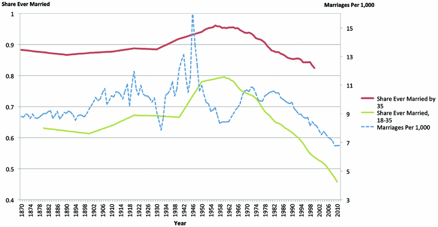
Figure 1. Different measures of marriage rates. Sources: IPUMS USA Census, 1880–1960; IPUMS CPS, 1962–2015; Vital Statistics of the United States; National Vital Statistics System, 100 years of Marriage and Divorce Statistics: United States, 1867–1967, Series 21, No. 24; U.S. Census Bureau, Statistical Abstract of the United States: 2012.
While the population-based and cross-sectional measures are constructed by calendar year, the cohort-based measure is constructed based on a cohort’s year of birth. To make all three measures comparable, and account for the fact that 35-year old married individuals were predominantly marrying in their twenties, we add 25 years to the cohort’s birth year and plot the cohort-based measure together with the other two.
It is immediately evident from Figure 1 that the three measures give different descriptions of the marriage rate in the United States over the past 140 years. The population-based measure is more volatile and characterized by big swings that are absent from the other two measures. In addition, in several periods, it displays patterns that contrast sharply with the evidence provided by the cross-sectional and cohort-based measures. For instance, after both world wars, the population-based measure shows a sudden and large increase in marriages followed by more than a decade of prolonged decline. One might infer that marriage rates increased sharply after the wars and then decreased steadily for about 15 years. But both the cross-sectional and cohort-based measures suggest that the marriage rates were roughly flat in the 15 years that followed World War I (WWI), and even increasing after World War II (WWII). Similarly, during the sixties and the first half of the seventies, the population-based variable displays rapid growth, which can be interpreted as a significant increase in marriage rates. The cross-sectional and cohort-based measures provide evidence, however, that this interpretation may be misleading, since during this period they document a decline in the share ever married.
Discrepancies between the population-based measure on one hand and the cross-sectional and cohort-based measures on the other should not come as a surprise, since an inspection of their definitions highlights that they describe different objects. The population-based measure, by construction, determines the share of individuals that enter a new marriage in a given year. The cross-sectional and cohort-based measures, instead, determine the share of individuals who are already married.
It should also not be surprising that the cross-sectional and cohort-based measures provide a similar description of marriage rates for most of the sample period. However, there are periods in which they converge or diverge. For example, starting in the early 1960s, the cross-sectional measure experiences a sharp drop suggesting that Americans are marrying at much lower rates with a drop from a peak of 79% in 1960 to 54% in 2000. The cohort-based measure displays a delayed and milder decline with marriage rates decreasing from a peak of 94% in 1960 to 79% in 2000.
The observed discrepancies between the different measures raise the question: Which one is better suited at characterizing marriage rates and their evolution? In the next two sections, we document that the answer depends on the research question. The evidence indicates that the cohort-based measure performs better when answering most of the questions economists are interested in. Nevertheless, there are cases in which the population-based measure outperforms the cohort-based measure and situations in which the cross-sectional measure is the best choice.
3. WHEN DOES THE COHORT-BASED MEASURE OUTPERFORM THE OTHER MEASURES?
In this section, we will provide evidence that the cohort-based measure is the best choice when a researcher is interested in computing the probability that a person marries during his or her life or fertile life, how this probability evolves, and how it differs across populations. This is the probability researchers need to evaluate how common marriage is in a period and over the years.
Suppose a researcher intends to answer the following question: Were people in the United States more likely to marry in the late thirties or in the late sixties? Figure 1 indicates that the answer varies depending on which measure is used. The population-based measure displays a drop between the two periods, suggesting that people were more willing to marry in the late thirties. The cross-sectional measure shows the opposite pattern with an increase between the two periods, suggesting that people were more willing to marry in the late sixties. The cohort-based measure provides still a different answer. Since this measure barely changes between the two periods, the researcher would conclude that people married at about the same rate.
To evaluate which measure provides the most credible answer, it is important to remember how they are constructed. The first measure, the number of marriages per 1,000 individuals, divides the number of new marriages that take place in a given year by the size of the population in that same year. The major limitation of this measure is that it is affected heavily by the fraction of individuals in the population that is of marriageable age in the period under investigation. In years in which marriageable-age individuals are over-represented, the population-based measure is high simply because they are the most likely to marry, even if the actual marriage rate is flat or declining. To document the effect of that demographic group, in Figure 2, we report the population-based measure and the number of people between the ages of 20 and 24 per 1,000 individuals. For most of the period, the population-based measure follows almost one-to-one the share of individuals of marriageable age. For example, the measure is high in the late 1960s and throughout the 1970s, when baby boomers entered marriageable age. Similarly, it is much lower in the 1950s and early 1960s than in the 1940s in part due to the decrease in individuals of marriageable age. In fact, during the fifties and sixties, individuals were marrying at record high rates, as we will show later in the paper. Because of this sensitivity to age structure, the population-based measure is not well suited for analyzing the evolution of the probability with which individuals ever marry. For the same reasons, it is also generally not well suited for international comparisons of marriage rates, despite its common use for such purposes.
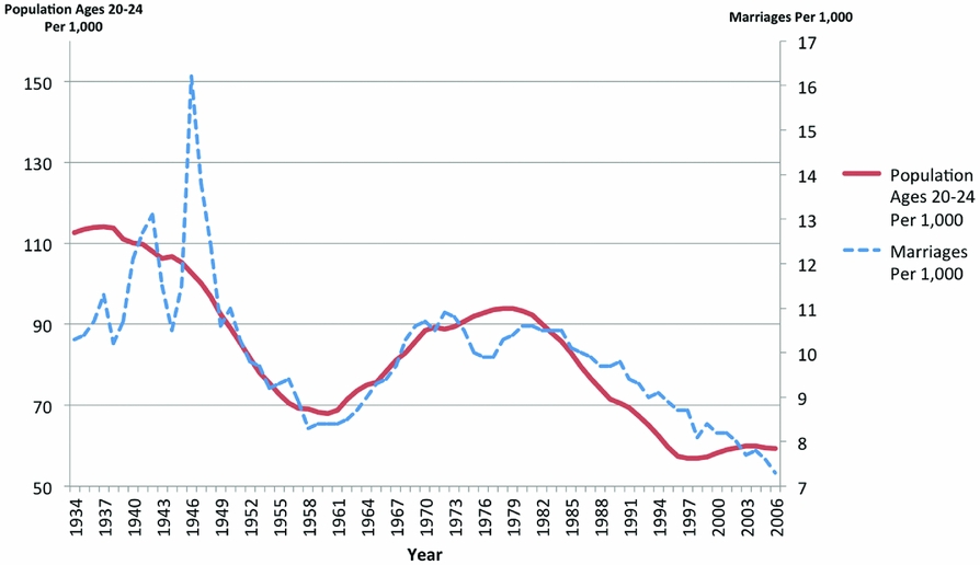
Figure 2. Marriages per 1,000 and the number of individuals aged 20–24 per 1,000. Yearly estimates of the population of individuals aged 20–24 are constructed using data on cohort size at birth from Vital Statistics of the United States, available starting with the 1909 birth cohorts, and retrieved from https://www.cdc.gov/nchs/data/statab/t941x01.pdf. Source: Vital Statistics of the United States.
Even in periods when the the fraction of individuals of marriageable age is relatively stable, the population-based measure has drawbacks. In particular, it is difficult to distinguish between temporary shifts in the timing of marriage, for example, due to war, and changes in the overall probability of marriage. For example, it is difficult to determine using this measure whether the large spike following WWII was simply the consequence of individuals postponing their marriages until after the end of the war, or whether in those years there was also an increase in the probability of ever marrying.
The other two measures are not affected by the limitations that characterize the population-based measure.Footnote 3 Then, why do the measures converge and diverge in certain periods, such as in the early 1940s or, starting in the 1960s, over the last several decades? For instance, the cross-sectional measure would suggest a sustained and sharp drop in marriage rates from the beginning of the sixties, whereas the cohort-based measure documents approximately constant marriage rates until 1970 and declining rates after that, though at a slower pace. The reason for these differences is that the cross-sectional measure is strongly affected by changes in the age at first marriage, which increased from a median age of around 20 years in 1960 to 24.5 years in 2000. To see the significant effect this can have on the cross-sectional measure, suppose that all cohorts are of the same size, and that in one period all individuals marry at age 21, while in another all individuals marry at age 25. In the first period, the cross-sectional marriage rate is equal to 83% (all individuals in the age range 21–35, divided by everyone between the ages of 18 and 35). In the second period, the marriage rate equals 61%. It therefore suggests a dramatic decline in marriage rates of 22 percentage points, even if the share that ever marry by 25 is still 100% in both cases. This example clarifies that the cross-sectional measure can potentially lead to incorrect inference in periods with significant changes in the age at first marriage, since it confounds the choice to delay marriage, for instance to complete one’s education, and the choice not to marry at all. Of course, the cohort-based measure may also be affected by changes in the age at first marriage if the age cut-off is too low. It is therefore important that one chooses it properly. If one believes that an age cut-off of 35 is too low—for example, because an increasing number of Americans choose to marry toward the end of their fertile lifespan—an age cut-off of 40 should be used.
To document that the concerns we have raised above are not only hypothetical, but have significant implications for relevant policy and research questions, we will consider two illustrative cases.
3.1. How Large Is the Racial Gap in Marriage?
To analyze the racial gap in marriage, we will consider the cross-sectional and cohort-based measures, since the marriages per 1,000 measure is not available by race. In Figure 3, we graph the two measures separately for Black and non-Hispanic White women. As Figure 3 shows, the size and evolution of the racial gap depend substantially on the measure employed. The cross-sectional measure suggests that, at least since 1990, White marriage rates have been dropping as rapidly as Black rates, with the racial gap remaining steady at around 18–20 percentage points. The cohort-based measure, on the other hand, documents a large, persistent divergence between Black and White marriage rate over the same period, with a much larger current gap of around 30 percentage points.

Figure 3. Share ever married 18–35 and share married by 35, by race. (A) Share ever married, 18–35. (B) Share ever married by 35. Sources: IPUMS USA Census, 1880–2000; IPUMS USA American Community Census, 2010.
How does one reconcile these two patterns? The two measures together indicate that for White individuals, the large drop in the cross-sectional measure largely reflects an increase in age at first marriage. Even though the cross-sectional measure is at a historical low for both White and Black Americans, Figure 3 shows that the cohort-based measure is almost as high today for White women as it was anytime between 1880 and 1940, prior to the unusually high marriage rates of the fifties and sixties. One can therefore conclude that White women are delaying marriage more than they did in the past, but continue to marry at high rates. By contrast, for Black women, the cohort-based measure is more than 30 percentage points lower today than it was any year before 1960. It is therefore possible to infer that the drop in the cross-sectional measure for that population reflects not only a delay in marriage, but also a steep decline in the probability of ever marrying, at least by 35.
To provide direct evidence for this explanation, in Figure 4, we graph for White and Black women the marriage hazard rate, which is defined as the probability that an individual of age a marries in a given year, conditional on entering the year single. It is constructed using the variable age at first marriage from the Census and CPS Fertility Supplements. In Figure 4 and all other figures containing the marriage hazard rate, we report the mean hazard rate, where the mean is computed across the relevant ages with all ages having equal weights.

Figure 4. Marriage hazards, by age and race. (A) White. (B) Black. The hazard rate is the probability that an individual of age a marries in year y, conditional on entering year y never married. We report the mean hazard rate over all a in each age group. The measure is constructed using an age at first marriage variable, available in the 1940, 1960, and 1980 Censuses. After 1980, we use the CPS June Fertility Supplement. The most recent CPS supplement with marital history variables is the 1995 supplement. Sources: IPUMS USA 1940, 1960, and 1980; IPUMS CPS June Fertility Supplement 1980–1983, 1986–1988, 1990, 1992, and 1995.
For White women, the marriage hazard for the age ranges 18–20 and 21–25 declines sharply starting around 1970. A few years later, the hazard rate for the age groups 26–30 and 31–35 begins to increase at a rate that largely compensates the decline for the two younger age ranges, indicating a delay in marriage. Interestingly, with the decline that started in the seventies, the hazard rate for White women 21–25 years returned approximately to pre-1940 levels. It is only the hazard rate for women 18–20 years that dropped below the pre-1940 levels, possibly due to a rising share of individuals attending college and postponing marriage until completion of their education. This explains why the cohort-based measure has remained high for White women, and fairly similar to the levels observed before 1940. By contrast, for Black women, the marriage hazard has declined for all age groups since the 1960s.
To conclude, since the cross-sectional measure conflates changes in age at first marriage with changes in the share that ever marry by 35, it appears to evolve similarly for Black and White women, but it reflects completely different marriage decisions and outcomes. The cohort-based measure is not affected by this limitation. It therefore better captures the size, nature of, and continuing divergence in the racial gap.
3.2. Has the Marriage Rate of White Women Decreased in the New Millennium?
Fairly consistent reporting in the popular press asserts that marriage rates for Americans across the board are declining in the new millennium to “record lows.”Footnote 4 How accurate is this description? Having already discussed the significant differences between Black and White marriage outcomes, and the downward trend in Black marriage rates, in this analysis, we will focus on the White population only.
Not surprisingly, the answer to whether marriage rates for White women declined significantly since 2000 depend strongly on the measure used. In Figure 5, we graph the cross-sectional measure for ages 18–35, and the cohort-based measure for different age cutoffs. Since 2000, the cross-sectional measure continues its steady decline, decreasing by about 10 percentage points over this period. If one takes that measure as a good description of the probability of marriage during an individual’s life or fertile life, the logical interpretation of the drop is that in the new millennium marriage has become a less popular institution.
The cohort-based measure indicates that this interpretation is misleading. If one uses a cutoff of 40, an age by which almost all individuals have made marriage decisions, the share ever married remains virtually flat over this period. If one uses a lower cutoff of 35, the drop in the cohort-based measure is around 4 percentage points. But even this decline appears to be driven primarily by lower marriage rates during the recession years starting in 2008. After 2012, the share ever married by 35 already appears to be increasing again. Interestingly, the cohort-based measure with a cutoff of 25, an age at which only a small fraction of people has made marriage decisions, replicates well the evolution of the cross-sectional measure. This confirms the main message provided in the second part of this section. The cross-sectional measure leads to misleading conclusions if used to characterize the probability of marriage in the last four decades, since large changes in age at first marriage confound its interpretation.
One may be concerned that in Figure 5 the cross-sectional and cohort-based measures consider different individuals. Cohorts who are 40 in 2015, for example, were 18–35 in the years 1993–2010; cohorts who are 40 in 2000 were 18–35 in the years 1978–1995. However, as Figure 3 A shows, these cohorts were 18–35 during years when the cross-sectional measure, which began its steep drop in 1960, was also declining. One can therefore conclude that White women today are continuing to delay marriage further, but that the share ever married by 35 or 40 has for now stabilized. Rather than being at a record low, the share of White women ever married by 40 (88.4%) was about as high in 2015 as it was during the period between 1880 and 1940 (88.6%, on average). In 2000, the share of White women ever married by 40 (about 90.5%) was in fact higher than in any other decennial year in the United States before 1950.
3.3. An Alternative Population-Based Measure
Now that we have described the effect of changes in age at first marriage on the marriage rate measures, we can discuss an alternative population-based measure that is frequently used, the number of marriages per 1,000 unmarried women 15 and older (or, in some cases, 18–64). This measure is used for example in the literature review by Greenwood et al. (Reference Greenwood, Guner and Vandenbroucke2017).
This measure is not as sensitive to the number of individuals of marriageable age as the variable number of marriages per 1,000 people. It has, however, the problem that it is affected by changes in age at first marriage, even more strongly than the cross-sectional measure. For example, consider a period in which everyone marries at age 20 and another in which all individuals marry at age 24. Assuming equally sized cohorts, in the first period marriages per 1,000 unmarried women 15 and older is equal to 200 (1,000 times the number of 20-year olds divided by the number of 15–19 year olds). In the second period, the measure is only 100 (1,000 times the number of 24-year olds divided by the number of 15–23 year olds). While this dramatic 50% drop in the measure might suggest a much lower propensity to marry in the population, the only change is a shift in the age at first marriage. With a more restrictive denominator, for instance unmarried women aged 18–64, the scale of the drop is even more dramatic.
To document the evolution of the two population-based measures considered in this paper, in Figure 6, we graph marriages per 1,000 and marriages per 1,000 unmarried women 15 and older. As expected, the measure marriages per 1,000 unmarried women drops rapidly after 1970 as the age at first marriage increases. This measure therefore suggests to researchers that the overall probability that a single woman marries today is at a record low, and around half of what it was before 1940. However, the previous example and the evidence we have provided on changes in the age at first marriage indicate that such an interpretation is misleading.
The discussion in this section indicates that the cohort-based measure outperforms the other measures if the objective is to evaluate the probability that an individual marries during his or her life or fertile life, or to compare this probability across time periods or populations. But there are instances in which the population-based and cross-sectional measures are better choices. The next section discusses those cases.
4. WHEN ARE THE POPULATION-BASED AND CROSS-SECTIONAL MEASURES GOOD CHOICES?
We start by considering situations where the population-based measures better describe marriage patterns. This class of measures outperforms the other two if one is interested in the fraction of the whole population that marries in a given year or in a set of years. Researchers and policy makers may be interested in this quantity, for instance, because it affects the labor and housing markets, and is predictive of possible fertility shocks. The population-based measures are also well suited to evaluate the effect of historical events that temporarily disrupt the functioning of the marriage market, such as wars. For example, Figure 6 documents a disruption in the marriage market during WWII in the form of a sharp decline in marriages per 1,000 and marriages per 1,000 unmarried women. It also shows that after the war, the marriage market resumed its standard way of functioning with the fraction marrying increasing rapidly to levels that are outliers if compared to other years in the sample period.
However, the drawbacks documented in the previous section affect the population-based measures even when they are used as a proxy for the probability with which single individuals marry in a given year. The number of marriages per 1,000 is highly sensitive to the number of marriageable-age individuals in the population and, therefore, to changes in age structure. The alternative measure, the number of marriages per 1,000 unmarried women, is affected by changes in age at first marriage.
One measure that we believe is better suited than the population-based measures to study the probabilities with which single individuals marry in different years is the marriage hazard, which we introduced earlier in the paper as the probability that an individual of age a marries in year y conditional on entering year y as never married. Since it is calculated for each age separately, not only is it not confounded by changes in age at first marriage, but it can be used to document those changes by reporting marriage hazards for different ages over time as we did in the previous section for Blacks and Whites. In addition, since it is constructed by age and year, the marriage hazard is not affected by changes in the age structure that may be generated, for instance, by an unusually large cohort of marriageable age. Last, the marriage hazard, unlike the population-based measures, can be constructed by race, ethnicity, age group, education, and other variables of interest. It can therefore be employed to document the evolution of the probability that a single individual marries in a given year for different populations.
To illustrate the advantages of the marriage hazard, in Figure 7, we report the evolution of that measure for the 18–25 and 26–35 age groups jointly with the evolution of the measure marriages per 1,000 individuals. The hazard rate captures well outlier years, such as during and immediately after WWII, just as the population-based measure does. Additionally, it correctly records the persistently high rate of marriage following the war, in line with the cross-sectional and cohort-based measures, and the sudden drop in marriage probabilities for the younger age group starting in 1970. The population-based measure cannot capture these patterns, since it is sensitive to the large drop in marriageable age individuals during the fifties, and to the increase in the number of such individuals during the seventies. Finally, the measure marriages per 1,000 declines continuously since 1980, obscuring the rise in marriage rates at higher ages, an important feature of the marriage market that generates probabilities of marriage today that are close to pre-1940 levels, a feature that is properly accounted for by the marriage hazard.
While we believe the marriage hazard is a better measure for comparing the probability with which single individuals marry in different years, care should be taken with this measure whenever it is reported as an average over an age range, as we do in this paper. The reason for this is that the average marriage hazard can be sensitive to how concentrated marriage is at specific ages. For example, take two populations in which the share ever married by 25 is 50%. In the first population, marriages are concentrated in one age: 50% of 18 year olds marry, and no marriages occur at ages 19–25. The marriage hazard is therefore 0.5 at age 18 and 0 at all other ages, for an average hazard rate of 0.063 over the age interval 18–25. In the second population, marriages are more disperse with all ages in the 18–25 interval having the same marriage hazard. In this case, all individuals between 18 and 25 have a hazard rate equal to 0.083, since (1 − 0.083)8 ≈ 0.5. In this example, the second population would have a higher reported average hazard rate for the age range 18–25, even though the share ever married by 25 is the same for both groups. In practice, marriage probabilities do tend to be more concentrated in some age groups than others, but are fairly evenly distributed within age groups that are sufficiently narrow. To be conservative, we have reported marriage hazards in Figure 4 for small (3-year or 5-year) age intervals. We find that larger age intervals, as in Figure 7, are also reliable, but researchers should keep in mind that this may depend on the population under study.
To complete our discussion of the marriage hazard, we note that this measure is closely related to the cohort-based measure, in that it captures annual changes in the share ever married by a given age. The relationship between these two measures can be used by researchers interested in studying the evolution of marriage rates over time. Indeed, when these two measures are presented jointly at corresponding ages, as in Figures 4 and 8, they provide a detailed annual snapshot of the marriage market, as they map out both the yearly stock of ever married individuals by a given age, and the rate at which these stocks are changing. Alternatively, if the focus is on comparing the lifecycle marriage behavior of two or more birth cohorts, a measure that can be used in conjunction with the hazard rate to study the marriage market is the cumulative distribution function (cdf) of the hazard rate. Figure 9 graphs this measure, which corresponds to the cohort-based measure graphed for each age cutoff.
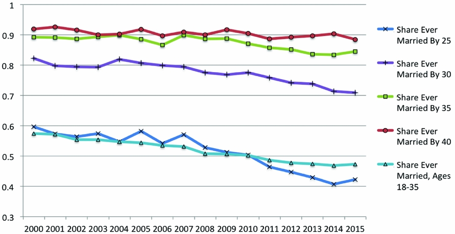
Figure 5. Share ever married, 2000–2015 (White). Source: IPUMS CPS, 2000–2015.
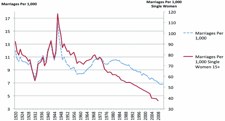
Figure 6. Marriages per 1,000 and marriages per 1,000 single women aged 15+. Sources: Vital Statistics of the United States.
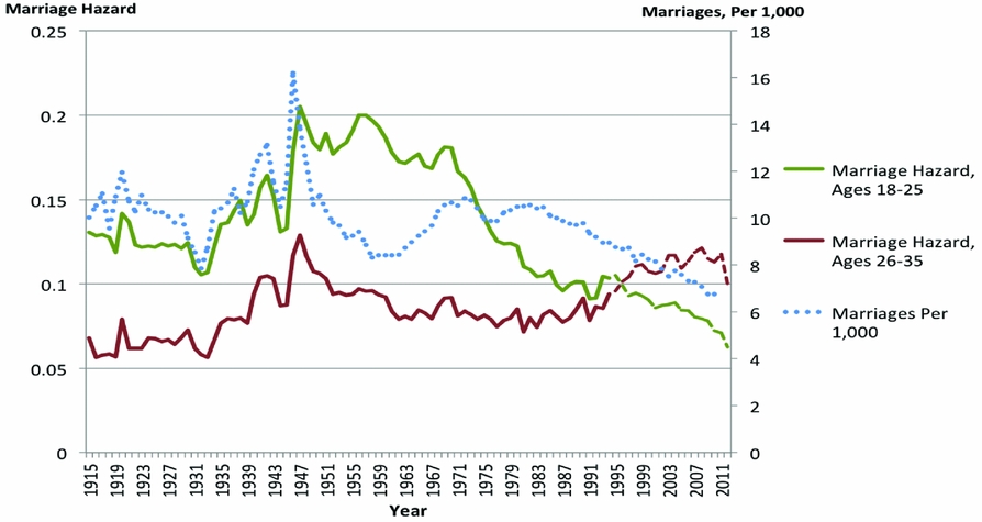
Figure 7. Marriages per 1,000 and marriage hazards. See notes in Figure 4. From 1915 to 1994, we use an age at first marriage variable to construct the marriage hazard measure, most recently available in 1995. After 1995, we construct a measure of the hazard rate using changes in share ever married for a given cohort over time, estimated using the March CPS. Sources: Vital Statistics of the United States; IPUMS USA 1940, 1960, and 1980; IPUMS CPS June Fertility Supplement 1980–1983, 1986–1988, 1990, 1992, and 1995; IPUMS CPS ASEC 1995–2015.
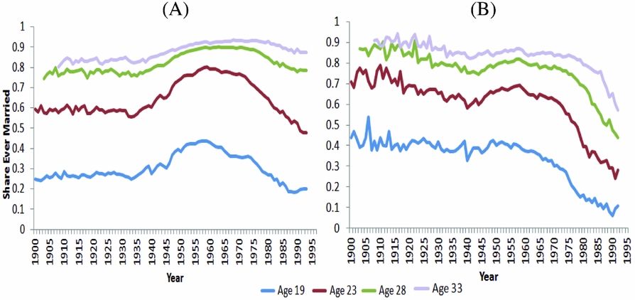
Figure 8. Share ever married, by age and calendar year. (A) White. (B) Black. Sources: IPUMS USA 1940, 1960, and 1980; IPUMS CPS June Fertility Supplement 1980–1983, 1986–1988, 1990, 1992, and 1995.
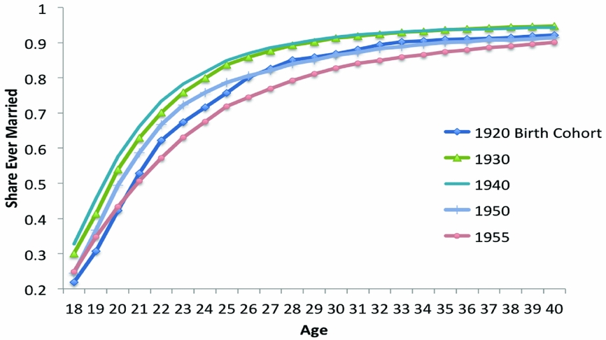
Figure 9. Share ever married by age (women). Sources: IPUMS CPS June Fertility Supplement 1980–1983, 1986–1988, 1990, 1992, and 1995.
We conclude the section by discussing situations in which the cross-sectional measure represents a better characterization of the marriage market. If one is interested in the fraction of people who are currently married, a cross-sectional measure is by definition the best choice. In this case, one should adjust the measure from share ever married to currently married in the age range of interest. This measure is useful when studying aggregate variables that are affected by the share of currently married households, such as aggregate labor force participation or aggregate expenditure and savings.Footnote 5 As Figure 1 indicates, if this is the objective of a researcher, the cohort-based measure produces misleading conclusions since it over-estimates the fraction who are currently in a marriage.
5. DISCUSSION AND IMPLICATIONS FOR FUTURE RESEARCH
How can better measures of marriage rates lead to further progress on questions related to marriage decisions? In this section, we provide three concrete suggestions. Given the expanding interest in economic drivers and consequences of marriage decisions [e.g., see recent review pieces by Stevenson and Wolfers (Reference Stevenson and Wolfers2007) and Greenwood et al. (Reference Greenwood, Guner and Vandenbroucke2017)], and calls for making studies of family formation and household decision-making a more integral part of research in macroeconomics [e.g., see the recent handbook chapter by Doepke and Tertilt (Reference Doepke and Tertilt2016)], we believe this discussion is particularly timely.
First, with better measures in hand, researchers can focus on more precise questions. The large fall in marriage rates suggested by the population-based and cross-sectional measures, especially relative to the fifties and sixties, has motivated many important studies about the “decline” of marriage. However, these measures paint an incomplete picture. The data indicate that the share ever married by 35 or 40 is about as high for White Americans in the 21st century as for the years prior to 1950.Footnote 6 The main difference relative to previous periods is that individuals now marry later: Marriage hazards indicate that White women in their late twenties or early thirties today marry at the same rates as women under 25 prior to the 1950s. Therefore, to understand drivers of and returns to marriage, at least for White Americans, we need studies that explain the temporarily high marriage rates mid-century, and the delay rather than decline of marriage today. We are only aware of a limited number of such studies [e.g., Goldstein and Kenney (Reference Goldstein and Kenney2001), Caucutt et al. (Reference Caucutt, Guner and Knowles2002), Doepke et al. (Reference Doepke, Hazan and Maoz2015)].
Second, the marriage hazard and cohort-based measures discussed in this paper make it possible to systematically compare marriage probabilities for racial, educational, and other subgroups. This is not true for aggregate variables such as the popular population-based measure or, alternatively, the comparison can lead to misleading results when using cross-sectional measures, as we showed for Black and White marriage rates. This feature of the marriage hazard and cohort-based measures allows also for sharper tests of hypotheses related to marriage formation, especially those based on aggregate statistics. For instance, though in the aggregate marriage measures may be negatively correlated with women’s labor force participation rates and positively correlated with fertility rates, the same relationships are not systematically observed for subpopulations. Highly educated women today, for example, are more likely to ever marry and stay married than lower-educated women, despite their higher labor force participation rates and lower fertility rates.
Finally, the less popular but more precise measures we have discussed in this paper, such as marriage hazards, offer details on the timing of changes in marriage probabilities of singles that are not available with other measures. This again provides valuable data for hypothesis testing. For example, sharp structural breaks in Figure 4 A, such as the steep drop in marriage probabilities beginning precisely in 1970, cannot be explained by forces affecting marriage that are more gradual in nature, such as changes in the wage structure [Gould and Paserman (Reference Gould and Paserman2003)] or the price of home technologies [Greenwood and Guner (Reference Greenwood and Guner2009)]. Instead, such sudden breaks are more consistent with a sharp policy change or the introduction of a new technology. The legalization of abortion in several large states in 1970 and nation-wide by 1973 [Myers (Reference Myers2017)] would appear to be a promising candidate to explain the sharp changes in marriage probabilities, which are particularly pronounced at younger ages. A second example is represented by the large and simultaneous increase in marriage probabilities for all age groups, even older women, in the mid- to late 1930s documented in Figure 4.Footnote 7 Accounting for this pattern requires an explanation for why marriage became more attractive for individuals of all ages during this period.
We conclude the paper by pointing out that we have focused on one particular subset of marriage behaviors—the decision to ever marry—mainly for expositional purposes. However, other marriage behaviors, such as divorce, have undergone significant changes over the last 50 years and are also of significant interest to researchers. Since statistics used to describe marriage and divorce are similarly constructed, our findings extend to studies relying on divorce rate measures. In particular, the most common measures of divorce rates—population-based measures such as divorces per 1,000, and cross-sectional measures such as share of individuals currently or ever divorced in a given age range—are characterized by similar drawbacks as their corresponding marriage measures. For these reasons, cohort-based measures of share ever divorced, as well as divorce hazards by age and year, are preferable for many research questions.
6. CONCLUSIONS
In this paper, we consider different measures of marriage rates and provide evidence that the two classes of measures typically used in the literature, the population-based and cross-sectional measures, generally lead to misleading inference when used to study the probability that someone married during his or her life or fertile life, its evolution, and differences across populations. An examination of the data indicates that an alternative measure, which we call the cohort-based measure, is not affected by the limitations that characterize the first two classes of measures. Alternatively, in cases when researchers are interested in year-on-year changes in marriage probabilities of singles rather than the share that ever marry, the data indicate that age-specific marriage hazards are more reliable than population-based measures. Therefore, these measures are better choices for researchers interested in studying marriage probabilities and their changes.


