


1. Introduction
Coated or encapsulated bubbles (EBs) have a large number of applications in the field of medical science, for targeted drug delivery (Tachibana & Tachibana Reference Tachibana and Tachibana1999; Unger et al. Reference Unger, Hersh, Vannan, Matsunaga and McCreery2001; Tsutsui, Xie & Porter Reference Tsutsui, Xie and Porter2004; Unger et al. Reference Unger, Porter, Culp, Labell, Matsunaga and Zutshi2004; Liu, Miyoshi & Nakamura Reference Liu, Miyoshi and Nakamura2006; Hernot & Klibanov Reference Hernot and Klibanov2008; Kooiman et al. Reference Kooiman, Vos, Versluis and de Jong2014), as contrast agents for ultrasound medical imaging (Hoff Reference Hoff2001; Stride & Saffari Reference Stride and Saffari2003; Lindner Reference Lindner2004; Postema et al. Reference Postema, Van Wamel, Lancée and De Jong2004; Klibanov Reference Klibanov2006), among others. Though EBs are widely used for ultrasound medical imaging, in particular, a recent study (Errico et al. Reference Errico, Pierre, Pezet, Desailly, Lenkei, Couture and Tanter2015) has shown that these bubbles can also be used as tracers to extract vascular geometry (microvascular imaging) and blood flow velocity over a large dynamic range in micron length scales. The shell material of such bubbles can be made up of polymers (Liu et al. Reference Liu, Zhou, Yang, Shen, Wang, Zhang, Zhi and Wu2014; Song et al. Reference Song, Peng, Xu, Wang, Yu, Hou, Zou and Yao2018), proteins (Wang et al. Reference Wang, Xue, Zhao, Qin, Zhang and Li2020) or phospholipids (Santos et al. Reference Santos, Morris, Glynos, Sboros and Koutsos2012; Abou-Saleh et al. Reference Abou-Saleh, Peyman, Critchley, Evans and Thomson2013; Li et al. Reference Li, Matula, Tu, Guo and Zhang2013; Gong, Cabodi & Porter Reference Gong, Cabodi and Porter2014; Parrales et al. Reference Parrales, Fernandez, Perez-Saborid, Kopechek and Porter2014; van Rooij et al. Reference van Rooij, Luan, Renaud, van der Steen, Versluis, de Jong and Kooiman2015; Lum et al. Reference Lum, Dove, Murray and Borden2016; Segers et al. Reference Segers, de Rond, de Jong, Borden and Versluis2016; Helfield Reference Helfield2019; Shafi et al. Reference Shafi, McClements, Albaijan, Abou-Saleh, Moran and Koutsos2019; Segers et al. Reference Segers, Gaud, Casqueiro, Lassus, Versluis and Frinking2020). Thus, experimental and theoretical understanding of the response of EBs to the external acoustic field is of great importance for the future developments of these promising applications.
Many experimental studies had been carried out to understand the behaviour of the EBs where different techniques have been used for oscillating the EBs. As the shell material parameters cannot be measured directly, such indirect experimental techniques or approaches are of greater importance in characterizing the shell material properties and studying the responses of the EBs. De Jong et al. (Reference de Jong, Hoff, Skotland and Bom1992) and de Jong & Hoff (Reference de Jong and Hoff1993) used bubble scattering phenomenon and mentioned that the scattering, absorption and extinction cross-section are vital acoustic properties of EBs, especially in echocardiographic applications. Many models were developed for describing the acoustic scatter and attenuation from suspensions of the EBs (Hoff, Sontum & Hoff Reference Hoff, Sontum and Hoff1996; Frinking & de Jong Reference Frinking and de Jong1998). Taking a step further, Morgan et al. (Reference Morgan, Allen, Dayton, Chomas, Klibaov and Ferrara2000) considered the echoes from wideband insonation, the effect of transmitted phase, and further compared with theoretical predictions by experimentally measuring the scattered pressure from a single EB. Back-scatter detection (Chang et al. Reference Chang, Shun, Wu and Levene1995; Shi et al. Reference Shi, Forsberg, Hall, Chiao, Liu, Miller, Thomenius, Wheatley and Goldberg1999; Basude & Wheatley Reference Basude and Wheatley2001) and high-speed photography (Dayton et al. Reference Dayton, Morgan, Klibanov, Brandenburger and Ferrara1999; de Jong et al. Reference de Jong, Frinking, Bouakaz, Goorden, Schourmans, Jingping and Mastik2000) has also been used to characterize and quantify the responses of EBs. The high-speed cameras are considered as a source of direct measurement of the EBs’ size. But inaccuracies have been observed in such measures due to the blurred edges of EBs. Gorce, Arditi & Schneider (Reference Gorce, Arditi and Schneider2000) performed a study on SonoVue® and determined the shell parameters from a comparison study of the model with that of experimental measurements of the attenuation coefficients. Experiments have also been carried out following the acoustic spectroscopy approach by transmitting a sequence of tone bursts within a range of frequencies (van der Meer et al. Reference van der Meer, Dollet, Voormolen, Chin, Bouakaz, de Jong, Versluis and Lohse2007; Helfield & Goertz Reference Helfield and Goertz2013). Tu et al. (Reference Tu, Guan, Qiu and Matula2009) performed experiments using light scattering methods to study the dynamical response of the EBs when subjected to an ultrasound field. Furthermore, they considered three different and popular shelled bubble dynamics models (de Jong & Hoff Reference de Jong and Hoff1993; Sarkar et al. Reference Sarkar, Shi, Chatterjee and Forsberg2005; Marmottant et al. Reference Marmottant, van der Meer, Emmer, Versluis, de Jong, Hilgenfeldt and Lohse2005) and tried to comment on the best bubble shelled model by fitting the experimental data. They estimated the shell parameters by fitting the experimental light scattering data with the linearized version of the Marmottant model and discussed the variation of shell elasticity modulus  $(\chi )$ and shell dilatational viscosity
  $(k^{S})$ with the initial radii of the bubble. In a detailed review, Versluis et al. (Reference Versluis, Stride, Lajoinie, Dollet and Segers2020) have highlighted the development of the EBs along with various experimental measuring methods.
For the theoretically developed EB models, one of the critical aspects is to inspect if the theoretical model is in good agreement with the experimental observations. It could be fitting the experimental time series response or estimating the shell properties such as shell elasticity modulus  $(\chi )$, shell dilatational viscosity
  $(k^{S})$, among others, though with some additional assumptions. Assuming the encapsulation as a thin shell, various researchers have developed mathematical models for contrast agent microbubbles. Complementing such shell models are the studies of de Jong et al. (Reference de Jong, Hoff, Skotland and Bom1992), de Jong & Hoff (Reference de Jong and Hoff1993), de Jong, Cornet & Lancée (Reference de Jong, Cornet and Lancée1994) and Church (Reference Church1995), who came up with a model by adding elastic and viscous terms of the shell into the Rayleigh–Plesset (RP) equation. de Jong et al. (Reference de Jong, Hoff, Skotland and Bom1992) also proposed a theoretical model to study the properties of contrast agent microbubbles where an elastic shell surrounds the air bubbles. The predictions of this theoretical model were proved to be promising when compared with transmission or experimental measurements. They assumed that the loss of transmission energy is due to the scattering of acoustic energy from the microbubble, thermal conduction within the microbubble and the viscosity of the surrounding fluid. But this model was better in describing the behaviour of larger bubbles than the smaller ones and predicted high scattering power and attenuation at higher frequencies. Further, de Jong & Hoff (Reference de Jong and Hoff1993) extended this model by considering the absorption due to frictional forces in the shell material. The fitting values of shell elasticity and friction parameters resulted in a calculated scatter power and were in good agreement with the scatter measurements. The shell model was also developed considering zero thickness interface bubble, performing an in vitro acoustic investigation for two different rheological models (Sarkar et al. Reference Sarkar, Shi, Chatterjee and Forsberg2005). They presented a detailed comparative study of various model behaviours and their ability to predict the experimental measurements. Dynamic simulation of lipid shelled microbubbles was carried out by Marmottant et al. (Reference Marmottant, van der Meer, Emmer, Versluis, de Jong, Hilgenfeldt and Lohse2005), referred to as the Marmottant model. These authors have studied the interface tension in an ad hoc manner, which is empirical but does not provide any relevant physical phenomenon. To resolve this, Paul et al. (Reference Paul, Katiyar, Sarkar, Chatterjee, Shi and Forsberg2010) considered interface strain-dependent surface tension with an interface elasticity constant. In the process of fitting the experimental data, these models (Marmottant et al. Reference Marmottant, van der Meer, Emmer, Versluis, de Jong, Hilgenfeldt and Lohse2005; Paul et al. Reference Paul, Katiyar, Sarkar, Chatterjee, Shi and Forsberg2010) assumed that some material properties of the shell material depend on initial bubble size. Models were also developed with the nonlinear theory for shell viscosity (Doinikov, Haac & Dayton Reference Doinikov, Haac and Dayton2009b), which depicted the dominant compression behaviour in encapsulated microbubbles. Some models (Qin & Ferrara Reference Qin and Ferrara2010) considered the shell elastic term valid for finite deformations, unlike the Church model (Church Reference Church1995), which is valid only for small deformations. Their model described the dynamics of contrast agents in vivo considering the effects of liquid compressibility (approximated to first order), the shell and the surrounding tissue. Tsiglifis & Pelekasis (Reference Tsiglifis and Pelekasis2008) developed an EB model, where the encapsulating shell was modelled as a thin membrane following hyperelastic constitutive laws. This model emphasized the flow structure aspect of radial bubble dynamics. Recently, Chabouh et al. (Reference Chabouh, Dollet, Quilliet and Coupier2021) developed an EB model where the bubble shell is considered to be a compressible viscoelastic isotropic material and was later generalized to an anisotropic material.
Though many EB models are limited to the study of radial oscillations, for an EB in an ultrasound field, the shape instabilities are equally important. Using optical imaging, such instabilities were even observed in experiments demonstrating the destruction of the bubble during compression (Chomas et al. Reference Chomas, Dayton, May, Allen, Klibanov and Ferrara2000). Motivated by these observations, many EB models were proposed to describe the non-spherical oscillations of EB dynamics (Versluis et al. Reference Versluis, van der Meer, Lohse, Palanchon, Goertz, Chin and de Jong2004; van der Meer et al. Reference van der Meer, Dollet, Goertz, de Jong, Versluis and Lohse2006; Dollet et al. Reference Dollet, van der Meer, Garbin, de Jong, Lohse and Versluis2008; Versluis et al. Reference Versluis, Goertz, Palanchon, Heitman, van der Meer, Dollet, de Jong and Lohse2010; Vos et al. Reference Vos, Dollet, Versluis and de Jong2011).
Steigmann & Ogden (Reference Steigmann and Ogden1999) developed a theory for coupled three-dimensional deformations of elastic solids with elastic films at their bounding surfaces. They proposed a simple theoretical derivation validating finite deformations and compatible with general mechanical principles. They assumed the film to be an elastic surface that resists the variations in its metric and curvature. This approach further opened ways to solve various complex technical problems, which included any isotropic substrates with hemitropic (defined in § 2.1) or isotropic films attached to the surfaces using the generalized kinematics of surfaces. Following the work of Steigmann & Ogden (Reference Steigmann and Ogden1999) and based on the results from other theoretical, experimental and computational studies supporting the size dependence of interface energy and interface stresses (Tolman Reference Tolman1949; Jiang & Lu Reference Jiang and Lu2008; Medasani & Vasiliev Reference Medasani and Vasiliev2009), Gao et al. (Reference Gao, Huang, Qu and Fang2014) proposed an interface theory which broadly explained the curvature dependence of interface energy and the effect of the residual elastic field on the bulk due to the interface energy. They described the deformation due to interface energy by hypothetically splitting the solid into homogeneous splits along the interface. They also emphasized the fact that this splitting is purely an imaginary action and, hence, named it a ‘fictitious stress-free configuration’, but it provided a valid explanation for the calculation of the residual elastic field due to the interface energy.
It is understandable that when an EB is suspended in a fluid, the interfaces between the gas-encapsulation and encapsulation-liquid carry sufficient surface or interface energy that significantly affects the mechanics. The influence of this interface energy on EB dynamics is not well studied in the existing models. Although models with interface strain are considered (Marmottant et al. Reference Marmottant, van der Meer, Emmer, Versluis, de Jong, Hilgenfeldt and Lohse2005; Paul et al. Reference Paul, Katiyar, Sarkar, Chatterjee, Shi and Forsberg2010) by directly adding it to the interface tension, these models do not capture the essential interface mechanics due to the lack of a proper continuum framework. However, recent literature shows the importance of deformation dependent surface or interface energy of polymeric glass, thin films and networks (Liang et al. Reference Liang, Cao, Wang and Dobrynin2018; Schulman et al. Reference Schulman, Trejo, Salez, Raphaël and Dalnoki-Veress2018; Rallabandi et al. Reference Rallabandi, Marthelot, Jambon-Puillet, Brun and Eggers2019), and the importance of interface stretch ratio and curvature effects in the liquid–vapour interface and growing droplet (Moody & Attard Reference Moody and Attard2003; Bruot & Caupin Reference Bruot and Caupin2016). It was reported that when the polymer network attains maximum stretch, the strain-dependent surface energy shows its significance in terms of surface stresses (Liang et al. Reference Liang, Cao, Wang and Dobrynin2018). Despite various shell models developed in the literature, a better understanding of EB dynamics is lacking, and a thermodynamically consistent model including interface effects is required to explain the physical origins of EB characteristic behaviour observed in the experiments (using high-speed imaging techniques). One such important characteristic is the ‘compression-only’ behaviour (de Jong et al. Reference de Jong, Emmer, Chin, Bouakaz, Mastik, Lohse and Versluis2007; Sijl et al. Reference Sijl, Overvelde, Dollet, Garbin, De Jong, Lohse and Versluis2011) where the EB compresses significantly compared with its expansion.
In this paper we try to address these questions by proposing an interface energy model for the dynamics of gas filled EB suspended in a fluid. As we are keener on studying the behaviour of EBs with a few microns radius, the effect of interface energy becomes more dominant. Notably, the present model considers these interface effects and makes this a robust model over the existing literature. Motivated by the general framework of Steigmann & Ogden (Reference Steigmann and Ogden1999), we assume that the interfaces are of a Steigmann–Ogden type (interfaces where the nonlinear continuum framework of Steigmann & Ogden (Reference Steigmann and Ogden1999) is used to describe them in terms of deformation gradient tensor and curvature tensor) and calculate the additional terms from the modified Young–Laplace equation for the radial dynamics of EB. For a bubble of  $2\,\mathrm {\mu }$m inner radius with
  $20$ nm thickness, we estimate the interface and usual material parameters at a particular excitation pressure and frequency by constructing a nonlinear constrained minimization problem for dominant compression behaviour. We further analyse various bubble configurations and study the contributions of the parameters introduced in the present model. The results show that interface stretch and bending rigidity induced bulk residual stress plays a dominant role in the mechanics of EBs with possible negative dynamic inner interface tension. Later, we attempt to compare the present model for
  $1.7\,\mathrm {\mu }$m,
  $1.4\,\mathrm {\mu }$m and
  $1\,\mathrm {\mu }$m radii bubbles with existing experimental data and identify the importance of interface parameters introduced in this work. With the proposed model, we show that size-independent shell viscoelastic properties can be estimated for Tu et al. (Reference Tu, Guan, Qiu and Matula2009) experimental data.
This paper is organized as follows. In § 2 a detailed mathematical model is presented for the radial dynamics of EB. In § 2.1 we introduce the concept of fictitious configuration through the interface energy model and obtain the additional terms in the interface tension due to the modified Young–Laplace equation. In § 2.2 we discuss the constitutive relations of the bulk and the fluid. In § 2.3 we obtain the governing equation for the radial dynamics of EB as a modified RP equation with additional terms due to the interface energy. In § 3 we introduce a constrained optimization procedure to estimate the interface and material parameters and present the numerical results and validation with experiments in § 4. The conclusions are given in § 5.
2. Mathematical model
An important step in modelling multiphase interfaces is to identify the surface or interface excess thermodynamic variables along with that of the bulk phase variables (Sagis Reference Sagis2014). One such explicit important variable is the interface curvature. In fact, interface curvature can have a significant implicit influence on other thermodynamic variables such as interface energy, chemical potential and surface charge density. We first present an interface energy model based on the interface strain and curvature in the following sections. Later, we obtain the governing differential equation for the radial dynamics of EBs with additional terms due to the interface energy.
2.1. Interface energy model
In the existing literature (Helfrich Reference Helfrich1973; Rangamani et al. Reference Rangamani, Benjamini, Agrawal, Smit, Steigmann and Oster2013; Argudo et al. Reference Argudo, Bethel, Marcoline and Grabe2016; Bian, Litvinov & Koumoutsakos Reference Bian, Litvinov and Koumoutsakos2020), modelling of cell membranes and lipid bi-layers is performed using Helfrich curvature energy which takes care of the bending energy through Gaussian curvature and spontaneous curvature. However, one cannot directly use Helfrich energy to model interfaces, which requires a generic framework to identify the structure of interface energy in terms of material symmetries. Also, it is important to note that these models are used to study the initial natural states of micro- or nanoscale structures. On the other hand, we are interested in modelling encapsulated microbubbles with the effect of residual fields developed due to the interface energy. Therefore, we follow the generic continuum framework developed in the previous work (Fung Reference Fung1977; Steigmann & Ogden Reference Steigmann and Ogden1999; Gao et al. Reference Gao, Huang, Qu and Fang2014) to incorporate the interface energy effects using the general notions of differential geometry (Itskov Reference Itskov2019; Steinmann Reference Steinmann2015).
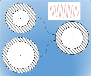
We assume that the bubble interface is a deformable mathematical surface compatible with the deformation of the bulk. We assume that there exist a bulk stress-free fictitious configuration (FC) of the bubble as shown in figure 1(a) with inner and outer radii,  $R_{e_1}$ and
  $R_{e_2}$, respectively. Even in the absence of external load this FC is unstable due to the presence of excess interface energy and the corresponding non-zero interface stress, which can force the bubble to attain a stable self-equilibrium state through expansion or shrinkage. This stable self-equilibrium state with bulk residual stress developed due to heterogeneous interface energy is shown in figure 1(b) with inner and outer radii
  $R_{10}$ and
  $R_{20}$, respectively. We also call this configuration a natural configuration (NC). Therefore, the bulk residual stress field in the bubble can be described as the state of self-equilibrium stress field due to the residual interface stresses. When excited by an external ultrasound pressure field, figure 1(c) represents the radial dynamic configuration (DC) of the same bubble with time-dependent inner and outer radii,
  $R_1(t)$ and
  $R_2(t)$, respectively.

Figure 1. Schematic representation of a gas filled encapsulated microbubble suspended in a viscous medium at three different configurations. (a) Fictitious (bulk stress-free) configuration (FC) of the bubble with possible expansion or shrinkage to reach the natural (static equilibrium) configuration (NC) in (b), and (c) Dynamic configuration (DC) of the bubble at an instant of time  $t$. (a) Fictitious configuration. (b) Natural configuration. (c) Dynamic configuration.
The approach presented above allows accounting for the influence of excess interfacial free energy and the corresponding non-zero residual interface stress on the mechanical behaviour of EBs. This FC is in agreement with the imaginary ‘fictitious stress-free configuration’ suggested by Gao et al. (Reference Gao, Huang, Qu and Fang2014). It is important to note that this FC may not exist physically. However, this assumption will help in calculating the bulk residual stress field induced by interfacial energy. Though many researchers have ignored the role of interfacial energy induced bulk residual stress, it should be noted that when we consider the effect of interface energy, the bulk residual stress field induced by the interfacial energy always becomes an important characteristic to account for and, hence, cannot be ignored. In very recent work, Chabouh et al. (Reference Chabouh, Dollet, Quilliet and Coupier2021) have also highlighted the importance of this stress-free configuration for developing dynamic models for EBs.
Let  $(x^{1},x^{2},x^{3})$ be the three-dimensional Cartesian coordinate system with unit basis vector triad as
  $(\boldsymbol {e}_1,\boldsymbol {e}_2,\boldsymbol {e}_3)$. Let
  $(\rho,\phi,\theta )$ be the principal spherical polar coordinates with unit basis vector triad
  $(\boldsymbol {e}_\rho,\boldsymbol {e}_\phi,\boldsymbol {e}_\theta )$. Here,
  $\rho$ is the radial coordinate from the centre of the bubble,
  $\phi$ is the polar angle formed with the
  $x^{3}$-axis and
  $\theta$ is the azimuthal angle measured about the
  $x^3$-axis in the counterclockwise direction from the
  $x^1$-axis. The relation between the Cartesian and the spherical polar coordinates is given by
 \begin{equation} \left. \begin{aligned} x^{1} & =\rho\sin\phi\cos\theta,\\ x^{2} & =\rho\sin\phi\sin\theta,\\ x^{3} & =\rho\cos\phi. \end{aligned} \right\} \end{equation}
The unit vectors along the three spherical coordinate directions are given by
 \begin{equation} \left. \begin{aligned} \boldsymbol{e}_\rho & =\sin\phi\cos\theta\,\boldsymbol{e}_1+\sin\phi\sin\theta\,\boldsymbol{e}_2+\cos\phi\,\boldsymbol{e}_3,\\ \boldsymbol{e}_\phi & =\cos\phi\cos\theta\,\boldsymbol{e}_1+\cos\phi\sin\theta\,\boldsymbol{e}_2-\sin\phi\,\boldsymbol{e}_3,\\ \boldsymbol{e}_\theta & ={-}\sin\theta\,\boldsymbol{e}_1+\cos\theta\,\boldsymbol{e}_2. \end{aligned} \right\} \end{equation}
For describing bulk radial motion of the bubble, we assume that  $\boldsymbol {x}_e=r_e \boldsymbol {e}_\rho$ as the position vector of a material point in the FC with radius
  $r_e$. Similarly, let
  $\boldsymbol {x}=r(r_e,t)\boldsymbol {e}_\rho$ be the position vector of a material point in the DC. Then the bulk deformation gradient tensor,
  $\boldsymbol{\mathsf{A}}$, and the corresponding left Cauchy–Green deformation tensor,
  $\boldsymbol{\mathsf{B}}$, can be expressed as (Itskov Reference Itskov2019)
 \begin{equation} \left. \begin{aligned} \boldsymbol{\mathsf{A}} & ={\partial\boldsymbol{x}}/{\partial \boldsymbol{x}_e}=\frac{\partial{r}}{\partial r_e}\boldsymbol{e}_\rho\otimes\boldsymbol{e}_\rho+\frac{r}{r_e}\boldsymbol{e}_\phi\otimes\boldsymbol{e}_\phi+\frac{r}{r_e}\boldsymbol{e}_\theta\otimes\boldsymbol{e}_\theta,\\ \boldsymbol{\mathsf{B}} & =\boldsymbol{\mathsf{A}}\boldsymbol{\mathsf{A}}^\textrm{T}=\left(\frac{\partial{r}}{\partial r_e}\right)^2\boldsymbol{e}_\rho\otimes\boldsymbol{e}_\rho+\left(\frac{r}{r_e}\right)^2\boldsymbol{e}_\phi\otimes\boldsymbol{e}_\phi+\left(\frac{r}{r_e}\right)^2\boldsymbol{e}_\theta\otimes\boldsymbol{e}_\theta, \end{aligned} \right\} \end{equation}
where  $\boldsymbol {c}\otimes \boldsymbol {d}$ represents the tensor product of two vectors
  $\boldsymbol {c}$ and
  $\boldsymbol {d}$.
Following the framework of Steigmann & Ogden (Reference Steigmann and Ogden1999), we idealize the gas-encapsulation and encapsulation-liquid interfaces as mathematical interfaces of zero thickness and call it Steigmann–Ogden interfaces (SOIs). Let  $\theta ^1=\phi$ and
  $\theta ^2=\theta$ be the surface coordinates of the spherical interface of radius say
  $r_0$. In the convected coordinate system, let
  $r(r_0,t)$ be the deformed radius of the interface. For the bubble undergoing spherical deformation, the principal stretch ratio
  $\lambda =r(r_0,t)/r_0$. Let
  $\boldsymbol Z(\theta ^1,\theta ^2)$ and
  $\boldsymbol z(\theta ^1,\theta ^2)$ be the position vectors of the same point on the undeformed and deformed interfaces, respectively, given by
 \begin{equation} \left. \begin{aligned} \boldsymbol Z(\theta^1,\theta^2) & =r_0(\sin\theta^1\cos\theta^2\,\boldsymbol{e}_1+\sin\theta^1\sin\theta^2\,\boldsymbol{e}_2+\cos\theta^1\,\boldsymbol{e}_3),\\ \boldsymbol z(\theta^1,\theta^2) & =r(r_0,t)(\sin\theta^1\cos\theta^2\,\boldsymbol{e}_1+\sin\theta^1\sin\theta^2\,\boldsymbol{e}_2+\cos\theta^1\,\boldsymbol{e}_3). \end{aligned} \right\} \end{equation}
Due to the deformation of the bulk of the bubble, the interface can be assumed to be convected and the deformation mapping,  $\boldsymbol \chi$, relates the same point before and after deformation as
 \begin{equation} \boldsymbol z(\theta^1,\theta^2)=\boldsymbol \chi(\boldsymbol Z(\theta^1,\theta^2)). \end{equation}
For the given position vectors of the interface, the tangent vectors  $\boldsymbol G_\alpha$ and
  $\boldsymbol g_\alpha$ on the undeformed and deformed interfaces, respectively, are calculated using
 \begin{equation} \boldsymbol{G}_\alpha=\boldsymbol{Z}_{,\alpha},\quad \boldsymbol{g}_\alpha=\boldsymbol{z}_{,\alpha},\quad \alpha\in\{1,2\},\quad ({\cdot})_{,\alpha}=\frac{\partial({\cdot})}{\partial\theta^\alpha}, \end{equation}
and the expressions for these vectors are given by
 \begin{gather} \boldsymbol{G}_1=r_0\,\boldsymbol{e}_\phi,\quad \boldsymbol{G}_2=r_0\sin\phi\,\boldsymbol{e}_\theta, \end{gather}
 \begin{gather}\boldsymbol{g}_1=r(r_0,t)\,\boldsymbol{e}_\phi,\quad \boldsymbol{g}_2=r(r_0,t)\sin\phi\,\boldsymbol{e}_\theta. \end{gather}
The components of the interface metric tensor for the undeformed and deformed interfaces, respectively, are given by
 \begin{gather} G_{\alpha\beta}=\begin{pmatrix} \boldsymbol{G}_1\boldsymbol{\cdot}\boldsymbol{G}_1 & \boldsymbol{G}_1\boldsymbol{\cdot}\boldsymbol{G}_2\\ \boldsymbol{G}_2\boldsymbol{\cdot}\boldsymbol{G}_1 & \boldsymbol{G}_2\boldsymbol{\cdot}\boldsymbol{G}_2 \end{pmatrix}=r_0^2\;{\textrm{{diag}}}(1,\sin^2\phi), \end{gather}
 \begin{gather}g_{\alpha\beta}=\begin{pmatrix} \boldsymbol{g}_1\boldsymbol{\cdot}\boldsymbol{g}_1 & \boldsymbol{g}_1\boldsymbol{\cdot}\boldsymbol{g}_2\\ \boldsymbol{g}_2\boldsymbol{\cdot}\boldsymbol{g}_1 & \boldsymbol{g}_2\boldsymbol{\cdot}\boldsymbol{g}_2 \end{pmatrix}=r(r_0,t)^2\;{\textrm{{diag}}}(1,\sin^2\phi) =\lambda^2 \it{G}_{\alpha\beta}. \end{gather}
For the given undeformed metric tensor components  $G_{\alpha \beta }$, the Christoffel symbols are defined as
 \begin{equation} \tilde{\varGamma}_{\alpha\beta}^\gamma=\tfrac{1}{2}G^{\gamma\delta}(G_{\alpha\delta,\beta}+G_{\delta\beta,\alpha}-G_{\beta\alpha,\delta}). \end{equation}
Similarly,  $\varGamma _{\alpha \beta }^\gamma$ are the Christoffel symbols constructed using the deformed interface metric tensor components
  $g_{\alpha \beta }$. The covariant derivative of a tensor generalizes the concept of partial derivative onto the curved surface. The following relation obtains the calculation of the components of the covariant derivative
  $(:)$ of a vector
  $(v^\alpha )$:
 \begin{equation} {v^\alpha}_{:\beta}={v^\alpha}_{,\beta}+\varGamma^\alpha_{\gamma\beta}\,v^\gamma. \end{equation}
The dual tangent vectors represented by  $\boldsymbol {G}^\alpha$ and
  $\boldsymbol {g}^\alpha$ associated with the coordinates
  $\theta ^\alpha$ are given by
 \begin{equation} \boldsymbol{G}^\alpha=G^{\alpha\beta}\boldsymbol{G}_\beta,\quad \boldsymbol{g}^\alpha=g^{\alpha\beta}\boldsymbol{g}_\beta. \end{equation}
The calculated values of the components of the dual metric tensors  $G^{\alpha \beta }$ and
  $g^{\alpha \beta }$, respectively, are obtained as
 \begin{gather} G^{\alpha\beta}=r_0^2\;\textrm{{diag}}(1,\csc^2\phi), \end{gather}
 \begin{gather}g^{\alpha\beta}=r(r_0,t)^2\;\textrm{{diag}}(1,\csc^2\phi)= \lambda^{-2}\, \it{G}^{\alpha\beta}. \end{gather}
The second fundamental forms  $Q_{\alpha \beta }$ and
  $q_{\alpha \beta }$ representing the normal curvatures associated with the deformed and the undeformed surfaces, respectively, are given by
 \begin{equation} Q_{\alpha\beta}=\boldsymbol{N}\boldsymbol{\cdot}\boldsymbol{G}_{\alpha:\beta},\quad q_{\alpha\beta}=\boldsymbol{n}\boldsymbol{\cdot}\boldsymbol{g}_{\alpha:\beta}. \end{equation}
Here,  $\boldsymbol {N}$ and
  $\boldsymbol {n}$ are the outward normal vectors to the undeformed and deformed interfaces, respectively, given by
 \begin{equation} \left. \begin{aligned} \boldsymbol{N} & =\tfrac{1}{2}\mu^{\alpha\beta}\boldsymbol{G}_\alpha\times\boldsymbol{G}_\beta,\\ \boldsymbol{n} & =\tfrac{1}{2}\varepsilon^{\alpha\beta}\boldsymbol{g}_\alpha\times\boldsymbol{g}_\beta,\quad\text{(summation convention)} \end{aligned} \right\} \end{equation}
where  $\varepsilon ^{\alpha \beta }=e^{\alpha \beta }/\sqrt {g}, \mu ^{\alpha \beta }=e^{\alpha \beta }/\sqrt {G}$ with
  $G=\textrm {det}(G_{\alpha \beta })=r_0^4\sin ^2\phi, g=\textrm {det}(g_{\alpha \beta })=r(r_0,t)^4\sin ^2\phi$ and
  $e^{\alpha \beta }=e_{\alpha \beta }$ is the alternator symbol (
 $e^{12}=-e^{21}=1, e^{11}=e^{22}=0$). Furthermore, we calculate the relations
 \begin{equation} \boldsymbol{G}_{1,1}={-}r_0\,\boldsymbol{e}_r,\quad \boldsymbol{G}_{1,2}=\boldsymbol{G}_{2,1}=r_0\cos\phi\,\boldsymbol{e}_\theta, \quad \boldsymbol{G}_{2,2}={-}r_0\sin\phi\,(\cos\theta\,\boldsymbol{e}_1+\sin\theta\,\boldsymbol{e}_2), \end{equation}
and obtain the expression for  $Q_{\alpha \beta }$ using the relations in (2.16a,b) and (2.17) where
  $\boldsymbol {N}=\boldsymbol {e}_\phi \times \boldsymbol {e}_\theta =\boldsymbol {e}_\rho$ as
 \begin{equation} Q_{\alpha\beta}={-}r_0\;\textrm{{diag}}(1,\sin^2\phi) ={-}{{r}}_0^{{-}1}{G}_{\alpha\beta}. \end{equation}
From the kinematics of the interface deformation, the deformation gradient tensor  $\boldsymbol{\mathsf{a}}$ can be written as (Itskov Reference Itskov2019)
 \begin{equation} \boldsymbol{\mathsf{a}}=\boldsymbol{g}_\beta\otimes\boldsymbol{G}^\beta. \end{equation}
The Jacobian  $(J)$ for the deformation is defined as the ratio of deformed to underformed interface areas, given by
 \begin{equation} J=\textrm{det}\,\boldsymbol{\mathsf{a}}=\sqrt{g/G}. \end{equation}
The right Cauchy-Green deformation tensor  ${\boldsymbol{\mathsf{C}}}$ is isotropic and can be expressed as
 \begin{equation} \boldsymbol{\mathsf{C}}=\boldsymbol{\mathsf{a}}^\textrm{T}\boldsymbol{\mathsf{a}}=g_{\alpha\beta}\boldsymbol{G}^\alpha\otimes\boldsymbol{G}^\beta. \end{equation}
The curvature tensor  $(\boldsymbol{\mathsf{q}})$ and the relative curvature tensor
  $(\boldsymbol {\kappa })$, related to the deformed and the undeformed configurations, respectively, are defined as
 \begin{equation} \left. \begin{aligned} \boldsymbol{\mathsf{q}} & =q_{\alpha\beta}\,\boldsymbol{g}^\alpha\otimes\boldsymbol{g}^\beta,\\ \boldsymbol\kappa & =\kappa_{\alpha\beta}\,\boldsymbol{G}^\alpha\otimes\boldsymbol{G}^\beta,\\ \end{aligned} \right\} \end{equation}
with the relation  $\boldsymbol \kappa =-\boldsymbol{\mathsf{a}}^\textrm {T}\boldsymbol{\mathsf{q}}\,\boldsymbol{\mathsf{a}}$. Then the relation between the components of the above two curvature tensors is
  $\kappa _{\alpha \beta }=-q_{\alpha \beta }$, where
  $q_{\alpha \beta }$ is calculated using (2.16a,b).
In a detailed study accounting for the material symmetry of the interface, Steigmann (Reference Steigmann2001) concluded that the interfacial energy is not an isotropic scalar-valued tensor function corresponding to the reference configuration, rather it is a function of the right Cauchy–Green interface deformation tensor  $\boldsymbol{\mathsf{C}}$ and the relative curvature tensor
  $\boldsymbol {\kappa }$. Here, the interface is assumed to be a micropolar, which is not isotropic with respect to inversion, also known as hemitropic. In other words, an interface whose symmetry group consists of all rotations but no reflections are said to be hemitropic. For such an hemitropic interface, its energy density is expressed as (Fung Reference Fung1977; Steigmann & Ogden Reference Steigmann and Ogden1999; Gao et al. Reference Gao, Huang, Qu and Fang2014)
 \begin{equation} \gamma=\gamma(\boldsymbol{\mathsf{C}},{\boldsymbol \kappa}), \end{equation}
and satisfies the relation
 \begin{equation} \gamma(\boldsymbol{\mathsf{C}},{\boldsymbol \kappa})=\gamma(\boldsymbol{\mathsf{Q}}\boldsymbol{\mathsf{C}}\boldsymbol{\mathsf{Q}}^\textrm{T},\boldsymbol{\mathsf{Q}}{\boldsymbol \kappa}\boldsymbol{\mathsf{Q}}^\textrm{T}), \end{equation}
where  $\boldsymbol{\mathsf{Q}}$ is a proper-orthogonal second-order tensor.
Hence, according to standard representation theory, the interface energy density can be expressed in terms of six basis invariants of the right Cauchy–Green interface deformation tensor  $\boldsymbol{\mathsf{C}}$, the relative curvature tensor
  $\boldsymbol {\kappa }$ and the permutation tensor density
  $\boldsymbol {\mu }$ on the undeformed interface as
 \begin{equation} \gamma=\gamma(I_1, I_2, I_3, I_4, I_5, I_6), \end{equation}
and the invariants are given by (see Appendix A)
 \begin{equation} \left. \begin{aligned} I_1 & =\textrm{tr}\,\boldsymbol{\mathsf{C}}=G^{\alpha\beta}C_{\alpha\beta},\\ I_2 & =\textrm{det}\,\boldsymbol{\mathsf{C}}=J^2=g/G,\\ I_3 & =\textrm{tr}{\,\boldsymbol \kappa}=G^{\alpha\beta}\kappa_{\alpha\beta},\\ I_4 & =\textrm{det}{\,\boldsymbol \kappa}=\tfrac{1}{2}\mu^{\alpha\beta}\mu^{\gamma\delta}\kappa_{\alpha\gamma}\kappa_{\beta\delta},\\ I_5 & =\textrm{tr}(\boldsymbol{\mathsf{C}}\boldsymbol{\kappa})=C_{\alpha\beta}\kappa^{\alpha\beta}=C^{\alpha\beta}\kappa_{\alpha\beta},\\ I_6 & =\textrm{tr}(\boldsymbol{\mathsf{C}}\boldsymbol{\kappa}\boldsymbol{\mu})=G_{\alpha\beta}C_{\gamma\delta}\kappa^{\alpha\gamma}\mu^{\beta\delta}=G_{\alpha\beta}\kappa_{\gamma\delta}C^{\alpha\gamma}\mu^{\beta\delta}. \end{aligned} \right\} \end{equation}
 The choice of these basis invariants are unique to hemitropic material property. These invariants mentioned above were first listed by Zheng (Reference Zheng1993) and further, the two-dimensional Cayley–Hamilton theorem can be used to obtain the equivalence of these invariants to that provided by Zheng. The expressions for the Cauchy interface stress  $(\boldsymbol \sigma )$ and the moment
  $({\boldsymbol{\mathsf{m}}})$ tensors are calculated using the relations (for detailed derivation see Steigmann & Ogden Reference Steigmann and Ogden1999; Gao et al. Reference Gao, Huang, Qu and Fang2014)
 \begin{equation} {\boldsymbol \sigma}=2\,\frac{\partial \gamma}{\partial{\boldsymbol{\mathsf{C}}}},\quad {{\boldsymbol{\mathsf{m}}}}=\frac{\partial\gamma}{\partial \boldsymbol \kappa}. \end{equation}
Using the expression for interface energy in terms of invariants, one can obtain the expressions for the components of interface stress tensor and the Eulerian bending moment tensor as
 \begin{equation} \left. \begin{aligned} \frac{1}{2}J\sigma^{\alpha\beta} & =\frac{\partial \gamma}{\partial I_1}G^{\alpha\beta}+ \frac{\partial \gamma}{\partial I_2}\tilde{C}^{\alpha\beta}+\frac{\partial \gamma}{\partial I_5}\kappa^{\alpha\beta}+\frac{1}{2}\frac{\partial \gamma}{\partial I_6}\left(D^{\alpha\beta}+D^{\beta\alpha}\right),\\ Jm^{\alpha\beta} & =\frac{\partial \gamma}{\partial I_3}G^{\alpha\beta}+ \frac{\partial \gamma}{\partial I_4}\tilde{\kappa}^{\alpha\beta}+\frac{\partial \gamma}{\partial I_5}C^{\alpha\beta}+\frac{1}{2}\frac{\partial \gamma}{\partial I_6}\left(E^{\alpha\beta}+E^{\beta\alpha}\right), \end{aligned} \right\} \end{equation}
where
 \begin{equation} D^{\alpha\beta}=G_{\gamma\delta}\mu^{\alpha\gamma}\kappa^{\beta\delta},\quad E^{\alpha\beta}=G_{\gamma\delta}\mu^{\alpha\gamma}C^{\beta\delta}. \end{equation}
Here,  $\tilde {\boldsymbol{\mathsf{C}}}$ and
  $\boldsymbol {\tilde {\kappa }}$ are the adjugate of
  $\boldsymbol{\mathsf{C}}$ and
  $\boldsymbol {\kappa }$, respectively, with components given by
 \begin{gather} \tilde{C}^{\alpha\beta}=(\textrm{tr}\,\boldsymbol{\mathsf{C}})G^{\alpha\beta}-C^{\alpha\beta}, \end{gather}
 \begin{gather}\tilde{\kappa}^{\alpha\beta}=(\textrm{tr}\,\boldsymbol{\kappa})G^{\alpha\beta}-\kappa^{\alpha\beta}. \end{gather}
We assume that the bubble undergoes deformation from a FC such that the bulk deformation tensor  $\boldsymbol{\mathsf{A}}$ is compatible with the interface deformation tensor
  $\boldsymbol{\mathsf{a}}$. From the balance of linear momentum, the general governing equation for the radial dynamics of the shell material and the outer liquid can be expressed in terms of the bulk stress field
  ${\boldsymbol{\mathsf{T}}}$ and velocity field
  $\boldsymbol {u}(r,t)$ as
 \begin{equation} \varrho\left[{\boldsymbol u}_{,t}+(\boldsymbol{u}\boldsymbol{\cdot}\boldsymbol{\nabla}){\boldsymbol u}\right]=\boldsymbol{\nabla}\boldsymbol{\cdot}{\boldsymbol{\mathsf{T}}}, \end{equation}
where  $\varrho$ is the density of the medium. Due to the existence of interface energy, the generalized Young–Laplace interface jump condition can be expressed in terms of interface stress and bending moment as (for detailed derivations, see Steigmann & Ogden Reference Steigmann and Ogden1999; Gao et al. Reference Gao, Huang, Qu and Fang2014)
 \begin{equation} [\![{\boldsymbol{\mathsf{T}}}]\!]\boldsymbol{\cdot n}=\left[(\sigma^{\alpha\beta}-m^{\lambda\alpha}q^{\beta}_{\lambda})\boldsymbol{g}_\beta+m^{\beta\alpha}_{\quad:\beta}\boldsymbol{n}\right]_{:\alpha}, \end{equation}
where the surface covariant derivative of a second-order tensor  $m^{\beta \alpha }_{:\beta }$ is given by the expression
 \begin{equation} m^{\beta\alpha}_{:\beta}=m^{\beta\alpha}_{,\beta}+m^{\delta\alpha}\,\varGamma^\beta_{\;\,\delta\beta}+m^{\beta\delta}\,\varGamma^\alpha_{\delta\beta}, \end{equation}
and  $[\![{\boldsymbol{\mathsf{T}}}]\!]$ is the jump in the stress due to interface energy. Similar to the calculations of
  $Q_{\alpha \beta }$ in (2.19), using the relations (2.10), (2.15) and (2.17), the expression for the curvature tensor are obtained for the inner (minus sign) and outer (plus sign) interfaces as
 \begin{equation} \left. \begin{aligned} q_{\alpha\beta} & ={-}({\mp} r(r_0,t)^{{-}1}g_{\alpha\beta})={-}({\mp} r_0^{{-}1}\lambda G_{\alpha\beta}),\\ q^\alpha_{\beta} & =g^{\alpha\gamma}q_{\beta\gamma}={-}({\mp} r_0^{{-}1}\lambda^{{-}1} \delta^\alpha_{\beta}), \end{aligned} \right\} \end{equation}
and the expressions for the components of the relative curvature tensor  $\boldsymbol {\kappa }$ are given by
 \begin{equation} \left. \begin{aligned} \kappa_{\alpha\beta} & ={\mp} r_0^{{-}1}\lambda G_{\alpha\beta},\\ \kappa^{\alpha\beta} & ={\mp} r_0^{{-}1}\lambda^3 g^{\alpha\beta}. \end{aligned} \right\} \end{equation}
Therefore, the contra- and co-variant components of the interface deformation tensor components can be written as
 \begin{equation} \left. \begin{aligned} C_{\alpha\beta} & =\lambda^2 G_{\alpha\beta},\\ C^{\alpha\beta} & =G^{\alpha\gamma}G^{\beta\delta}C_{\gamma\delta}=\lambda^4g^{\alpha\beta}. \end{aligned} \right\} \end{equation}
The invariants in (2.27) are calculated as
 \begin{equation} I_1=2\,\lambda^2, \quad I_2=\lambda^4, \quad I_3=\mp2\,\lambda/r_0, \quad I_4=\lambda/r_0^2, \quad I_5=\mp2\,\lambda^3/r_0, \quad I_6=0. \end{equation}
 For the undeformed interface configuration, the identity tensor (unit tensor)  $\boldsymbol{\mathsf{1}}$ is given by
 \begin{equation} \boldsymbol{\mathsf{1}}=G_{\alpha\beta}\,\boldsymbol{G}^\alpha\otimes\boldsymbol{G}^\beta. \end{equation}
Using the identity tensor one can write  $\boldsymbol{\mathsf{C}}=\lambda ^2\boldsymbol{\mathsf{1}}$ and the components of the adjugate of
  $\boldsymbol{\mathsf{C}}$ are
  $\tilde {C}^{\alpha \beta }=C^{\alpha \beta }.$ From the relations in (2.29), components of interface stress and Eulerian bending moment tensors, respectively, can be simplified to yield the relations
 \begin{equation} \sigma^{\alpha\beta}=\sigma g^{\alpha\beta},\quad m^{\alpha\beta}=m g^{\alpha\beta}, \end{equation}
where
 \begin{gather} \sigma=\gamma_0+2\left(\gamma_1+\gamma_2\lambda^2\mp\frac{\gamma_5\lambda}{r_0}\right), \end{gather}
 \begin{gather}m=\gamma_3\mp\frac{\gamma_4\lambda}{r_0}+\gamma_5\lambda^2, \end{gather}
with ‘ $-$’ and ‘
 $+$’ signs are supposed to be used for the inner and outer interfaces, respectively. Here, deformation independent interface tension is introduced as
  $\gamma _0$, and
  $\gamma _i=\partial \gamma /\partial I_i, i=1,2,$ are considered as interface material parameters. The generalized Young–Laplace equation (2.34) for the radial dynamics can be expressed as
 \begin{equation} [\![{\boldsymbol{\mathsf{T}}}]\!]\boldsymbol{\cdot} {\boldsymbol n}={-}({\mp} 2 r_0^{{-}1}\lambda^{{-}1}\varSigma)\;\boldsymbol{n}, \end{equation}
where  $\varSigma =\sigma \mp r_0^{-1}\lambda ^{-1}\,\textrm {m}$. The residual interface stress and bending moment tensors at static equilibrium are calculated by the substitution
  $\lambda =1$, which yields
  $\sigma ^{*\alpha \beta }=\sigma ^*g^{\alpha \beta }$ and
  $m^{*\alpha \beta }=m^*g^{\alpha \beta }$, where
  $\sigma ^*$ and
  $m^*$ are given by
 \begin{gather} \sigma^*=\gamma_0+2\left(\gamma_1+\gamma_2\mp\frac{\gamma_5}{r_0}\right), \end{gather}
 \begin{gather}m^*=\gamma_3+\gamma_5\mp\frac{\gamma_4}{r_0}. \end{gather}
Here, the assumption of  $\gamma _i=\partial \gamma /\partial I_i$ as constant gives a simple linear structure to the interface energy density function with a linear combination of the basis invariants defined in (2.27). However, in a more general case, the interface energy can be a nonlinear function of these basis invariants. Therefore, there is always scope to improve and modify the mathematical structure of the Young–Laplace equation and the residual stress field.
Comparing the residual stress  $\sigma ^*$ at the interface with two leading-order terms of well-known Tolman's formula (Tolman Reference Tolman1949)
  $\sigma _s\sim \sigma _\infty (1-2\delta _\infty /r_0)$ for a curved interface indicates that
  $\gamma _5$ has the role of Tolman's length scale
  $\delta _\infty$. In
  $\varSigma$,
  $\gamma _3$ appears to have a similar interpretation to
  $\gamma _5$ for
  $\lambda =1$; however, it is important to identify the distinct effects of
  $\gamma _3$ and
  $\gamma _5$ on the interface tension, as will be shown in (2.53).
As mentioned earlier, the present model naturally introduces residual stress in the bulk due to the expansion or shrinkage of the bubble after preparation, which was also observed in the experiments (de Jong et al. Reference de Jong, Emmer, Chin, Bouakaz, Mastik, Lohse and Versluis2007). This also indicates the important feature of equivalent NC bubbles with the same radii and internal gas pressure at the NC, which can show completely different mechanical behaviour. This behaviour is strongly connected to the process of attaining NC, which in-turn is related to the interface energy induced residual stress. On the other hand, one would also expect that different size bubbles made of the same shell material should demonstrate the behaviour based on same material constants. Here, we demonstrate these features by considering the above interface energy and corresponding interface parameters in the mathematical model of EB dynamics.
2.2. Constitutive relation for the shell and the fluid
We analyse the EB dynamics by assuming that the shell material and the fluid surrounding the bubble are homogeneous, isotropic and incompressible materials. Furthermore, the shell is assumed to be viscoelastic. A Kelvin–Voigt type constitutive model with elastic part described by the Mooney–Rivlin (MR) material model with elastic constants  $C_1$ and
  $C_2$, and a viscous part by the Newton's law of viscosity is considered. In order to capture the material nonlinearity of the shell material, we have chosen this basic nonlinear material model. The ratio
  $C_2/C_1$ in the MR material model is usually interpreted as a strain-softening or hardening parameter depending on its value. For an incompressible bulk MR material, the strain energy density
  $W=C_1(\tilde {I}_1-3)+C_2(\tilde {I}_2-3)$, where
  $\tilde {I}_1,\;\tilde {I}_2,\;\tilde {I}_3$ are the three invariants of
  ${\boldsymbol{\mathsf{B}}}$ given by
 \begin{equation} \left. \begin{aligned} \tilde{I}_1 & =\textrm{tr}{\,{\boldsymbol{\mathsf{B}}}}=2\varLambda^2+\varLambda^{{-}4},\\ \tilde{I}_2 & =\textrm{tr}{\,{\boldsymbol{\mathsf{B}}}^2}=2\varLambda^{{-}2}+\varLambda^4,\\ \tilde{I}_3 & =\textrm{det}\,{\boldsymbol{\mathsf{B}}}=1, \end{aligned} \right\} \end{equation}
where  $\varLambda =r/r_e$ is the principal stretch ratio in both
  $\theta ^1$ and
  $\theta ^2$ directions. Since the bulk is assumed to be incompressible,
  ${\tilde {I}}_3=1$ gives
 \begin{equation} \frac{\partial{r}}{\partial r_e}=\left(\frac{r_e}{r}\right)^2=\varLambda^{{-}2}. \end{equation}
Using superscripts  $S$ and
  $L$ for the shell and liquid parameters, respectively, the Cauchy stress tensor for the shell is given by
 \begin{equation}
{\boldsymbol{\mathsf{T}}}^{S}={-}p^{S}{\boldsymbol{\mathsf{I}}}+2(C_1+\tilde{I}_1C_2){\boldsymbol{\mathsf{B}}}-2C_2{\boldsymbol{\mathsf{B}}}^2+\eta^{S}[\boldsymbol{\nabla}\boldsymbol{u}^{S}+(\boldsymbol{\nabla}\boldsymbol{u}^{S})^\textrm{T}],
\end{equation}
\begin{equation}
{\boldsymbol{\mathsf{T}}}^{S}={-}p^{S}{\boldsymbol{\mathsf{I}}}+2(C_1+\tilde{I}_1C_2){\boldsymbol{\mathsf{B}}}-2C_2{\boldsymbol{\mathsf{B}}}^2+\eta^{S}[\boldsymbol{\nabla}\boldsymbol{u}^{S}+(\boldsymbol{\nabla}\boldsymbol{u}^{S})^\textrm{T}],
\end{equation}
where  $\eta ^{S}$ is the shell viscosity coefficient,
  $\boldsymbol{\mathsf{I}}$ is the identity tensor and
  $p^{S}$ is commonly referred to as the arbitrary hydrostatic pressure due to incompressibility. The liquid viscous stress tensor with viscosity coefficient
  $\eta ^{L}$ is given by the constitutive equation
 \begin{equation} {\boldsymbol{\mathsf{T}}}^{L}={-}p^{L}{{\boldsymbol{\mathsf{I}}}}+\eta^{L}[\boldsymbol{\nabla}\boldsymbol{u}^{L}+(\boldsymbol{\nabla}\boldsymbol{u}^{L})^\textrm{T}]. \end{equation}
2.3. Governing equation
For the radial dynamics of the shell exerted by an ultrasound field and the surrounding liquid, the governing equation in spherical polar coordinates with  $(r,\phi,\theta )$ as principal coordinate directions can be reduced to the radial equation
 \begin{equation} \varrho\left(\frac{\partial u}{\partial t}+{u}\frac{\partial u}{\partial r}\right)=\frac{\partial T_{rr}}{\partial r}+\frac{2 T_{rr}-T_{\phi\phi}-T_{\theta\theta}}{r}. \end{equation}
The stress jump conditions at the inner and outer interfaces are
 \begin{equation} \left. \begin{aligned} \left. T_{rr}^{S}\right\lvert_{r=R_1}+p_{g} & =\frac{2\sigma_1}{R_1},\\ \left[T_{rr}^{S}-T_{rr}^{L}\right]_{r=R_2} & ={-}\frac{2\sigma_2}{R_2}, \end{aligned} \right\} \end{equation}
where  $\sigma _1$ and
  $\sigma _2$ are the interface tension parameters given by
 \begin{equation} \left. \begin{aligned} \sigma_1 & =\gamma_{10}+2\left(\gamma_{11}+\gamma_{12}\frac{R_1^2}{R_{10}^2}-\gamma_{15}\frac{R_1}{R_{10}^2}\right)-\frac{1}{R_1}\left(\gamma_{13}-\gamma_{14}\frac{R_1}{R_{10}^2}+\gamma_{15}\frac{R_1^2}{R_{10}^2}\right),\\ \sigma_2 & =\gamma_{20}+2\left(\gamma_{21}+\gamma_{22}\frac{R_2^2}{R_{20}^2}+\gamma_{25}\frac{R_2}{R_{20}^2}\right)+\frac{1}{R_2}\left(\gamma_{23}+\gamma_{24}\frac{R_2}{R_{20}^2}+\gamma_{25}\frac{R_2^2}{R_{20}^2}\right), \end{aligned} \right\} \end{equation}
with  $\gamma _{i(\cdot )}, i=1,2$ correspond to the inner and outer interfaces, respectively. Unlike existing shell models, interface tensions are considered on either side of the bubble shell and dependent on the interface radius.
Substituting  $R_1=R_{10}$ and
  $R_2=R_{20}$ in the stress jump conditions in (2.52), one can rewrite the interface conditions at the NC of the bubble as
 \begin{gather} \left. T_{rr}^{S}\right\lvert_{R_1=R_{10}}+p_{g_0}=\frac{2}{R_{10}}\left[\gamma_{10}+2\left(\gamma_{11}+\gamma_{12}-\frac{\gamma_{15}}{R_{10}}\right)-\frac{1}{R_{10}}\left(\gamma_{13}-\frac{\gamma_{14}}{R_{10}}+\gamma_{15}\right)\right], \end{gather}
 \begin{gather}\left. T_{rr}^{S}\right\lvert_{R_2= R_{20}}\left.-T_{rr}^{L}\right\lvert_{R_2=R_{20}}\,{=}\,\frac{-2}{R_{20}}\left[\gamma_{20}\,{+}\,2\left(\gamma_{21}\,{+}\,\gamma_{22}\,{+}\,\frac{\gamma_{25}}{R_{20}}\right)\,{+}\,\frac{1}{R_{20}}\left(\gamma_{23}+\frac{\gamma_{24}}{R_{20}}\,{+}\,\gamma_{25}\right)\right]. \end{gather}
To obtain the governing equation, integrating (2.51) with respect to the radial coordinate  $r$ for the shell and liquid regions separately, we have
 $$\begin{gather} \int_{R_1}^{R_2} \varrho^{S}\left(\frac{\partial u^{S}}{\partial t}+{u^{S}}\frac{\partial u^{S}}{\partial r}\right) \,\textrm{d}r+\int_{R_2}^{\infty} \varrho^{L}\left(\frac{\partial u^{L}}{\partial t}+{u^{L}}\frac{\partial u^{L}}{\partial r}\right) \,\textrm{d}r \nonumber\\ = \int_{R_1}^{R_2} \left(\frac{\partial T^{S}_{rr}}{\partial r}+\frac{2T_{rr}^{S}-T^{S}_{\phi\phi}-T^{S}_{\theta\theta}}{r}\right) \,\textrm{d}r+\int_{R_2}^\infty \left(\frac{\partial T^{L}_{rr}}{\partial r}+\frac{2T^{L}_{rr}-T^{L}_{\phi\phi}-T^{L}_{\theta\theta}}{r}\right) \,\textrm{d}r, \end{gather}$$
where the superscripts  $S$ and
  $L$ represent the physical terms corresponding to the shell and liquid, respectively. From (2.49) we calculate the expressions for the components of the Cauchy stress tensor for the shell as
 \begin{equation} \left. \begin{aligned} T^{S}_{rr} & ={-}p^{S}+2\lambda^{{-}4}C_1+4\lambda^{{-}2}C_2+2\eta^{S}\left(\frac{\partial u^{S}}{\partial r}\right),\\ T^{S}_{\phi\phi} & =T^{S}_{\theta\theta}={-}p^{S}+2\lambda^{2}C_1+2(\lambda^4+\lambda^{{-}2})C_2+2\eta^{S}\left(\frac{u^{S}}{r}\right),\\ T^{S}_{r\phi} & =T^{S}_{\phi\theta}=T^{S}_{\theta r}=0. \end{aligned} \right\} \end{equation}
Similarly from (2.50), we calculate the components of the liquid viscous stress tensor as
 \begin{equation} \left. \begin{aligned} T^{L}_{rr} & ={-}p^{L}+2\eta^{L}\left(\frac{\partial u^{L}}{\partial r}\right),\\ T^{L}_{\phi\phi} & =T^{L}_{\theta\theta}={-}p^{L}+2\eta^{L}\left(\frac{u^{L}}{r}\right),\\ T^{L}_{r\phi} & =T^{L}_{\phi\theta}=T^{L}_{\theta r}=0. \end{aligned} \right\} \end{equation}
Using the above expressions for the stress components normal to the three principal coordinate planes and the expression for the velocity field in Appendix B, the governing equation for the radial dynamics of a bubble exerted by an ultrasound field is given by
 $$\begin{gather} \varrho^{S}\left[R_1\ddot{R}_1+\frac{3}{2}\dot{R}_1^2\right]-\left(\varrho^{S}-\varrho^{L}\right)\left[R_2\ddot{R}_2+\frac{3}{2}\dot{R}_2^2\right]=p_g-p_0-p_d+p_e-\frac{2\sigma_1}{R_1}-\frac{2\sigma_2}{R_2}\nonumber\\ -4\eta^{L}\frac{\dot{R}_2}{R_2}-4\eta^{S}\left(\frac{\dot{R}_1}{R_1}-\frac{\dot{R}_2}{R_2}\right), \end{gather}$$
where  $p_g$ is the gas pressure,
  $p_0$ is the ambient pressure,
  $p_d=p_a\sin (2{\rm \pi} f t)$ is the external acoustic field with pressure
  $p_a$ and frequency
  $f$, and
  $p_e$ is the elastic restoring force (see Appendix C) given by
 \begin{align}
p_e&={-}4\left[C_1\left(\frac{1}{4\varLambda_2^4}+\frac{1}{\varLambda_2}\right)+C_2\left(\frac{1}{2\varLambda_2^2}-\varLambda_2\right)\right]\nonumber\\&\quad +4\left[C_1\left(\frac{1}{4\varLambda_1^4}+\frac{1}{\varLambda_1}\right)+C_2\left(\frac{1}{2\varLambda_1^2}-\varLambda_1\right)\right].
\end{align}
\begin{align}
p_e&={-}4\left[C_1\left(\frac{1}{4\varLambda_2^4}+\frac{1}{\varLambda_2}\right)+C_2\left(\frac{1}{2\varLambda_2^2}-\varLambda_2\right)\right]\nonumber\\&\quad +4\left[C_1\left(\frac{1}{4\varLambda_1^4}+\frac{1}{\varLambda_1}\right)+C_2\left(\frac{1}{2\varLambda_1^2}-\varLambda_1\right)\right].
\end{align}
Here,  $\varLambda _1=R_1/R_{e_1}$ and
  $\varLambda _2=R_2/R_{e_2}$ are the stretch ratios. The interface tension parameters
  $(\sigma _1,\sigma _2)$ and the elastic restoring force
  $(p_e)$ are the additional terms which makes the governing equation (2.59) different from that of Church's model (Church Reference Church1995). When the bubble is in its NC the time-dependent terms in the governing equation vanish and the static equilibrium equation is given by
 \begin{align} p_{g_0}&=p_0+\frac{2}{R_{10}}\left[\gamma_{10}+2\left(\gamma_{11}+\gamma_{12}-\frac{\gamma_{15}}{R_{10}}\right)-\frac{1}{R_{10}}\left(\gamma_{13}-\frac{\gamma_{14}}{R_{10}}+\gamma_{15}\right)\right]\nonumber\\ &\quad +\frac{2}{R_{20}}\left[\gamma_{20}+2\left(\gamma_{21}+\gamma_{22}+\frac{\gamma_{25}}{R_{20}}\right)+\frac{1}{R_{20}}\left(\gamma_{23}+\frac{\gamma_{24}}{R_{20}}+\gamma_{25}\right)\right]\nonumber\\ &\quad +4\left[C_1\left(\frac{1}{4\varLambda_{20}^4}+\frac{1}{\varLambda_{20}}\right)+C_2\left(\frac{1}{2\varLambda_{20}^2}-\varLambda_{20}\right)\right]\nonumber\\ &\quad -4\left[C_1\left(\frac{1}{4\varLambda_{10}^4}+\frac{1}{\varLambda_{10}}\right)+C_2\left(\frac{1}{2\varLambda_{10}^2}-\varLambda_{10}\right)\right]. \end{align}
Let  $p_{g_e}$ be the uniform gas pressure inside the bubble in the FC. Assuming that the gas inside the bubble is undergoing expansion or compression with polytropic expansion index
  $k=1.4$, the relation between
  $p_g,p_{g_0}$ and
  $p_{g_e}$ can be expressed as
 \begin{equation} p_g=p_{g_0}\left(\frac{R_{10}}{R_1}\right)^{3k}=p_{g_e}\left(\frac{R_{e_1}}{R_1}\right)^{3k}. \end{equation}
With the inner and outer radii of the bubble at NC being known, the bubble radii at FC can be found by solving the nonlinear algebraic equation (2.61).
As we are interested in bubbles of radius  ${O}(10^{-6})$ m and thickness
  ${O}(10^{-9})$ m, inspecting the terms in (2.53), it is reasonable to assume the order of parameters
  $\gamma _{10},\gamma _{20},\gamma _{11},\gamma _{21},\gamma _{12},\gamma _{22}$ as
  ${O}(1)\,\textrm {N}\,\textrm {m}^{-1}$,
  $\gamma _{13},\gamma _{23},\gamma _{15},\gamma _{25}$ as
  ${O}(10^{-6}$ )N and
  $\gamma _{14},\gamma _{24}$ as
  ${O}(10^{-12})$ N m. Primarily this assumption ensures that the effective interface tension parameters
  $\sigma _1$ and
  $\sigma _2$ possess reasonable values of
  ${O}(1)\,\textrm {N}\,\textrm {m}^{-1}$. Also, it is worth mentioning that the order of these interface parameters are chosen such that it will not lead to large deviations in the bubble radii while undergoing deformation from the FC to the NC. In the rest of the paper,
  $\varrho ^{S}=1100\,\textrm {kg}\,\textrm {m}^{-3}$,
  $\varrho ^{L}=1000\,\textrm {kg}\,\textrm {m}^{-3}$,
  $\gamma _{10}=0.04\,\textrm {N}\,\textrm {m}^{-1}$,
  $\gamma _{20}=0.005\,\textrm {N}\,\textrm {m}^{-1}$ (Krasovitski & Kimmel Reference Krasovitski and Kimmel2006; Shao & Chen Reference Shao and Chen2015) and a numerical value of
  $\gamma _{ij}$ by default carries these orders apart from any other explicitly mentioned factors.
In (2.53),  $\gamma _{i2}$ term retains the effect of relative interface area. However, in the present model, the dynamic interface tension cannot become zero due to the change in the interface area, unlike the other models (Paul et al. Reference Paul, Katiyar, Sarkar, Chatterjee, Shi and Forsberg2010). On the other hand, both
  $\gamma _{13}$ and
  $\gamma _{15}$ can make the dynamic interface tension negative at the inner interface, which is purely an effect of interface bending rigidity. These relations also show distinct effects of
  $\gamma _3$ and
  $\gamma _5$ terms when the interface starts deforming. It is interesting to observe that the contribution of
  $\gamma _5$ terms in (2.59) is only through static equilibrium pressure and depends only on the initial size of the bubble. On the other hand, the dynamic interface tension has terms proportional to the interface radius and curvature through
  $\gamma _5$ and
  $\gamma _3$, respectively, which shows distinct effects.
Here, we study the influence of three important interface parameters  $\gamma _2,\gamma _3$ and
  $\gamma _5$ on the EB's NC and radial dynamics. These three interface parameters are related to the deformation dependent interface area, curvature and the coupling between the two. To understand the influence of these aspects further, we have constructed a multistart optimization problem by defining a compression or expansion ratio to estimate the interface and material parameters.
3. Constrained optimization
Let  $R_2^{ max}$ and
  $R_2^{ min}$ be the maximum and minimum outer radii, respectively, of the steady state response of a bubble at a particular excitation pressure and frequency. The compression or expansion ratio can be defined as
 \begin{equation} \zeta =\frac{R_2^{ max}-R_{20}}{R_{20}-R_2^{ min}}. \end{equation}
Here,  $\zeta \ll 1 (\gg 1)$ represents the compression (expansion) dominant behaviour of a bubble.
Based on typical compression dominant radial dynamics observed in the experiments at a specific range of excitation pressure and frequency (Doinikov & Bouakaz Reference Doinikov and Bouakaz2011), suitable parameters are estimated by setting up an minimization problem with parameters  $C_1,C_2,\eta ^{L},\eta ^{S},f,$ and
  $\gamma _{ij}, i=1,2, j=1$ to
  $5,$ as
 \begin{equation} \left. \begin{aligned} \text{Minimize:} & \quad \zeta, \\ \text{Constraints:} & \quad \zeta \leq \zeta_0,\;0.5 \leq \zeta_0 \leq 1,\\ & \quad\tilde{R}_{e_1}\geq 0.75,\tilde{R}_{e_2} \leq 0.95\ (\text{Case I}:\ \text{expanding bubble}),\\ & \quad \tilde{R}_{e_1}\geq 1.05,\tilde{R}_{e_2} \leq 1.25\ (\text{Case II}:\ \text{shrinking bubble}). \end{aligned} \right\} \end{equation}
Here,  $\zeta _0$ is the compression ratio obtained for a bubble attaining equivalent NC without interface energy and
  $\tilde {R}_{e_i}=R_{e_i}/R_{10}$ is the non-dimensional inner
  $(i=1)$ and outer
  $(i=2)$ radii of the bubble in the FC. We have solved the optimization problem using Matlab® R2018a (9.4.0) multistart optimization.
The above optimization problem is solved with proper nonlinear constraints for a bubble of  $2\,\mathrm {\mu }$m radius
  $(R_{10})$ with
  $20$ nm thickness
  $(h)$. The interface and material parameters are estimated for dominant compression behaviour, which will be discussed in the results § 4.1. Here, the shell thickness and other shell properties are chosen, referring to the agent bubble OptisonTM(Krasovitski & Kimmel Reference Krasovitski and Kimmel2006; Shao & Chen Reference Shao and Chen2015).
To fit the experimental data (de Jong et al. Reference de Jong, Emmer, Chin, Bouakaz, Mastik, Lohse and Versluis2007; van der Meer et al. Reference van der Meer, Dollet, Voormolen, Chin, Bouakaz, de Jong, Versluis and Lohse2007; Doinikov, Haac & Dayton Reference Doinikov, Haac and Dayton2009a; Tu et al. Reference Tu, Guan, Qiu and Matula2009) for thin lipid monolayer EBs, we set up another minimization problem with parameters  $C_1,C_2,\eta ^{L},\eta ^{S},f,p_{g_0},h$ and
  $\gamma _{ij}, i=1,2, j=1$ to
  $5,$ as
 \begin{equation} \left. \begin{aligned} \text{Minimize:} & \quad \zeta, \\ \text{Constraints:} & \quad (\zeta)_{LL} \leq \zeta \leq (\zeta)_\textit{UL}, \\ & \quad (R_2^{ min})_{LL} \leq R_2^{ min} \leq (R_2^{ min})_\textit{UL}. \end{aligned} \right\} \end{equation}
The values of  $\zeta$ and
  $R_2^{ min}$ are first identified from the experimental time series data. Using these values as a reference in the optimization problem, the constraints for
  $\zeta$ and
  $R_2^{ min}$ are modified close to experimental observations to estimate the interface and material parameters. In (3.3),
  $(\cdot )_{LL}$ and
  $(\cdot )_{\textit{UL}}$ correspond to the lower and upper limit values for these constraints, respectively. The results pertaining to these simulations will be discussed in § 4.2.
In all of these simulations, the lower and upper bounds for the interface parameters  $\gamma _{ij}, i=1,2, j=1$ to
  $5,$ are fixed within small intervals, based on their orders as discussed earlier towards the end of § 2.3.
4. Results and discussion
4.1. Analysis of various bubble configurations
A bubble can attain its NC by shrinkage or expansion from a stress-free configuration as shown in figure 1. Let  $\varLambda _{10}=R_{10}/R_{e1}$ be the pre-stretch at the inner interface with
  $\varLambda _{10} < 1 (>1)$ for the bubble attaining equilibrium NC by shrinking (expanding). For a given set of optimized interface parameters and material parameters with assumed equilibrium gas pressure,
  $p_{g_0}$, one can obtain the equation for static (natural) equilibrium from (2.59), which has a unique solution for the FC radii. Change in any of the interface parameter data possibly leads to a different FC, compression or expansion ratio, and pre-stress in the bulk. However, both these data represent equivalent NC if we assume that the amount of gas inside the bubble is the same. Therefore, we compare such configurations to understand the influence of interface parameters on the bubble dynamics through compression or expansion ratio and pre-stress.
Tables 1 and 2 contain representative data of interface and material parameters obtained from the optimization for compression dominant behaviour. It is interesting to note that interface energy induced bulk residual stress has an important role in the compression dominant behaviour. To identify the dominant interface parameters of table 1 data, bubbles with an equivalent NC obtained from different FCs are compared in table 3 by removing the contribution of specific interface parameters in the model. Data in table 3 suggests that  $\gamma _{i5}$ and
  $\gamma _{i2}$
  $(i=1,2)$ have significant contributions for dominant compression. For instance, in case II, setting
  $\gamma _{i5}=0$ requires an increase in the FC radii with
  $\zeta =1.02$, which is an expansion dominant behaviour. On the other hand, setting
  $\gamma _{i2}=0$ shows a decrease in the FC radii but still an increase in the value of
  $\zeta$. In the absence of interface energy, we have found an expanding FC in both the cases with
  $\zeta _0=0.69$ and
  $0.78$, respectively. However, we exclude such cases because modelling of such interfaces is incomplete without interface energy. This discussion shows that the nature of interface energy induced pre-stress in the bulk influences the compression or expansion ratio (
 $\zeta$) and is highly dependent on the interface parameters. Similar dominance of
  $\gamma _{i5}$ and
  $\gamma _{i2}$ are also found for a bubble attaining NC from a FC (data not presented here). Another important feature observed in figure 2 for the above data is the negative and positive dynamic inner interface tensions for case I and case II, respectively, as expected from (2.53). In this case, physically possible negative dynamic interface tension can be interpreted in terms of interface bending rigidity.


Table 1. Optimized interface parameters (IP) such as  $(\gamma _{11},\gamma _{21},\gamma _{12},\gamma _{22})\,\textrm {N}\,\textrm {m}^{-1}$,
  $(\gamma _{14},\gamma _{24})$ Nm and
  $(\gamma _{13},\gamma _{23},\gamma _{15},\gamma _{25})$ N for a bubble with
  $R_{10}=2\,\mathrm {\mu }$m, thickness
  $h=20$ nm, NC pressure
  $p_{g_0}=0.3$ MPa and excitation pressure
  $p_a=0.1$ MPa. Cases I and II correspond to a bubble undergoing expansion and shrinkage, respectively, from a fictitious to natural configuration.

Table 2. Optimized material parameters (MP) such as shell elastic constants  $(C_1,C_2)$ MPa, viscosity of shell
  $(\eta ^{S})$ Pa s and liquid
  $(\eta ^{L})$ mPa s, frequency
  $(f)$ MHz, compression ratios
  $\zeta$ and
  $\zeta _0$ for a bubble with
  $R_{10}=2\,\mathrm {\mu }$m, thickness
  $h=20$ nm, NC pressure
  $p_{g_0}=0.3$ MPa and excitation pressure
  $p_a=0.1$ MPa. Cases I and II correspond to a bubble undergoing expansion and shrinkage, respectively, from a fictitious to natural configuration.

Table 3. Values of compression ratio ( $\zeta$), inner (
 $R_{e_1}$) and outer (
 $R_{e_2}$) radii (
 $\mathrm {\mu }$m) of the bubble in a FC with the absence of specific interface parameters (IP)
  $(\gamma _{ij},i=1,2$ and
  $j=2\;\rm {to}\;5)$,
  $(\gamma _{11},\gamma _{21},\gamma _{12},\gamma _{22})\,\textrm {N}\,\textrm {m}^{-1}$,
  $(\gamma _{14},\gamma _{24})$ Nm and
  $(\gamma _{13},\gamma _{23},\gamma _{15},\gamma _{25})$ N from table 1.

4.2. Comparison with experimental data
To fit the experimental radius–time curves of EBs, NC gas pressure,  $p_{g_0}$, and bubble thickness,
  $h$, are two important quantities apart from all the interface and material parameters. Their roles become significantly important as they provide an idea about how the bubble shell was produced or fabricated, as identified and discussed by Chabouh et al. (Reference Chabouh, Dollet, Quilliet and Coupier2021). For a
 $1.7\,\mathrm {\mu }$m radius bubble, we modify the optimization problem with additional constraints
  $1.45< R_{2}^{ min}<1.5$ and optimization parameter,
  $p_{g_0}$. Referring to van der Meer et al. (Reference van der Meer, Dollet, Voormolen, Chin, Bouakaz, de Jong, Versluis and Lohse2007), the thickness of the EB is considered to be
  $4$ nm and
  $\eta ^{L}$ is taken as
  $2$ mPa s. On a similar note, for a
  $1.4\,\mathrm {\mu }$m and
  $1\,\mathrm {\mu }$m radius bubble, we modify the optimization problem with additional constraints
  $0.85< R_{2}^{ min}<0.9$ and
  $0.9< R_{2}^{ min}<0.95$, respectively, and optimization parameters,
  $p_{g_0}$ and
  $h$. Additionally, in these simulations we include a constraint for shear modulus
  $(\mu )$ such that
  $15\leq \mu \,({\rm MPa})\leq 17$ (referring to the agent bubble OptisonTM). The optimized interface and material parameters thus obtained are listed in tables 4 and 5, respectively. We have fitted the experimental radius–time data for a
  $1.7\,\mathrm {\mu }$m (van der Meer et al. Reference van der Meer, Dollet, Voormolen, Chin, Bouakaz, de Jong, Versluis and Lohse2007),
  $1.4\,\mathrm {\mu }$m (Doinikov et al. Reference Doinikov, Haac and Dayton2009a) and
  $1\,\mathrm {\mu }$m (de Jong et al. Reference de Jong, Emmer, Chin, Bouakaz, Mastik, Lohse and Versluis2007) radius bubble with the present model using these optimized interface and material parameters.
Table 4. Optimized interface parameters (IP) such as  $(\gamma _{11},\gamma _{21},\gamma _{12},\gamma _{22})\,\textrm {N}\,\textrm {m}^{-1}$,
  $(\gamma _{14},\gamma _{24})$ Nm and
  $(\gamma _{13},\gamma _{23},\gamma _{15},\gamma _{25})$ N for a bubble with a NC outer radius
  $R_{20}=1.7\,\mathrm {\mu }$m,
  $1.4\,\mathrm {\mu }$m and
  $1\,\mathrm {\mu }$m.

Table 5. Optimized material parameters (MP) such as shell elastic constants  $(C_1,C_2)$ MPa, viscosity of shell
  $(\eta ^{S})$ Pa s and liquid
  $(\eta ^{L})$ mPa s, frequency
  $(f)$ MHz, NC gas pressure
  $(p_{g_0})$ MPa, bubble thickness
  $(h)$ nm, compression ratios
  $\zeta$ and
  $\zeta _0$ for a bubble with a NC outer radius
  $R_{20}=1.7\,\mathrm {\mu }$m,
  $1.4\,\mathrm {\mu }$m and
  $1\,\mathrm {\mu }$m.

For a  $1.7\,\mathrm {\mu }$m radius bubble, we fitted the experimental radius–time data (van der Meer et al. Reference van der Meer, Dollet, Voormolen, Chin, Bouakaz, de Jong, Versluis and Lohse2007) with the Gaussian tapered 8-cycle acoustic pulse (as assumed in the experiments) of a bubble from the present model at
  $p_a=0.04$ MPa and
  $f=2.5$ MHz, as shown in figure 3(a). The results shown in figure 3(a) illustrate that the present model provides the best fit with the experimental data in the central region and shows deviations at the beginning and end stages, which is in good agreement with results reported by Tu et al. (Reference Tu, Guan, Qiu and Matula2009). However, it is important to note that the experiments for the
  $1.7\,\mathrm {\mu }$m bubble are conducted in a confined environment with possible near-wall effects (van der Meer et al. Reference van der Meer, Dollet, Voormolen, Chin, Bouakaz, de Jong, Versluis and Lohse2007). The near-wall effect could be one of the reasons for the mismatch between the experimental and theoretical data at the extreme ends of the Gaussian pulse. Though the present model is able to match the central region of the time series data for the
  $1.7\,\mathrm {\mu }$m bubble in figure 3(a), the material constants obtained from the fitting are underestimated (Payne et al. Reference Payne, Illesinghe, Ooi and Manasseh2005; van der Meer et al. Reference van der Meer, Dollet, Voormolen, Chin, Bouakaz, de Jong, Versluis and Lohse2007), because a solid surface near an oscillating bubble can introduce asymmetry and influence the radial oscillations and the amplitude. For a
  $1.4\,\mathrm {\mu }$m radius bubble, the experimental radius–time data are fitted with the 20-cycle acoustic pulse for a bubble from the present model at
  $p_a=0.1$ MPa and
  $f=3$ MHz, as shown in figure 3(b). For a
  $1\,\mathrm {\mu }$m radius bubble, the experimental radius–time data are fitted with the 6-cycle sine-wave burst at
  $p_a=0.1$ MPa and
  $f=1.8$ MHz, as depicted in figure 3(c). The optimized values of interface parameters represented in table 4 correspond to the bubble undergoing expansion from fictitious to natural configuration. In line with the conclusion drawn earlier for a
  $2\,\mathrm {\mu }$m bubble, we observed the possibility of negative dynamic inner interface tension for these cases as well.

Figure 3. Comparison of present model estimation with experimental radius–time curves (de Jong et al. Reference de Jong, Emmer, Chin, Bouakaz, Mastik, Lohse and Versluis2007; van der Meer et al. Reference van der Meer, Dollet, Voormolen, Chin, Bouakaz, de Jong, Versluis and Lohse2007; Doinikov et al. Reference Doinikov, Haac and Dayton2009a) for (a)  $1.7\,\mathrm {\mu }$m radius bubble with Gaussian tapered 8-cycle acoustic pulse at
  $p_a=0.04$ MPa and
  $f=2.5$ MHz; (b)
  $1.4\, \mathrm {\mu }$m radius bubble with 20-cycle acoustic pulse at
  $p_a=0.1$ MPa and
  $f=3$ MHz; (c)
  $1\,\mathrm {\mu }$m radius bubble with 6-cycle sine-wave burst at
  $p_a=0.1$ MPa and
  $f=1.8$ MHz.
De Jong et al. (Reference de Jong, Hoff, Skotland and Bom1992) emphasized that a bubble encapsulated with an elastic shell behaves differently from that of a bubble without encapsulation. They also pointed out that the bubble shell is characterized by a shell parameter given by  $S_p=Eh/(1-\nu )$, where
  $E$ is the Young's modulus,
  $\nu$ is the Poisson's ratio and
  $h$ is the shell thickness. Subsequently, the well-known Marmottant model (Marmottant et al. Reference Marmottant, van der Meer, Emmer, Versluis, de Jong, Hilgenfeldt and Lohse2005) introduced the shell elasticity modulus,
  $\chi =S_p/2$, and studied the bubble behaviour by taking into consideration the physical properties of the bubble coating. The shell elasticity modulus
  $(\chi )$ can be related to the shear modulus
  $(\mu )$ under thin-shelled elasticity theory as
  $\chi \,(\textrm {N}\,\textrm {m}^{-1})=3\,\mathrm {\mu }\textit {h}$ (Boal Reference Boal2002; Tu et al. Reference Tu, Guan, Qiu and Matula2009; Li et al. Reference Li, Matula, Tu, Guo and Zhang2013). This expression can also be obtained by substituting
  $E=2\mu (1+\nu )$ and
  $\nu =0.5$ (assuming rubber-like materials) in the expression of
  $S_p$. In the present model, the shell elastic constants
  $(C_1,C_2)$ from the MR material model are related to the shear modulus
  $(\mu )$ by the relation
  $\mu =2(C_1+C_2)$. Similarly, the dilatational viscosity of the shell
  $(k^{S})$ can be expressed in terms of viscosity of the shell
  $(\eta ^{S})$ and the shell thickness
  $(h)$ as
  $k^{S}\,(\textrm {kg}\,\textrm {s}^{-1})=3\,\eta ^{S}{h}$ (Tu et al. Reference Tu, Guan, Qiu and Matula2009).
In the available literature researchers have reported that the viscoelastic properties of the EBs are dependent on their initial size of the EB. Motivated by these observations, we estimate the interface  $(\gamma _{ij},i=1,2,j=1\ \textrm {to}\ 5)$ and material
  $(C_1,C_2,\eta ^{S},p_{g_0},h)$ parameters for various NC outer radii
  $(R_{20})$ of the bubble ranging from
  $0.8$ to
  $3.25\,\mathrm {\mu }$m at
  $p_a=0.15$ MPa and
  $f=2.5$ MHz. This estimated interface and material parameters are tabulated in the supplementary material available at https://doi.org/10.1017/jfm.2021.979 and used in the subsequent analysis (figures 4 and 5). In these simulations we modify the constraints for
  $\zeta$ and
  $R_{2}^{ min}$ and set it close to their calculated values at the respective bubble radii using the linearized Marmottant model to be in good agreement with Tu et al. (Reference Tu, Guan, Qiu and Matula2009) experimental time series data.

Figure 4. Calculated values of shell elasticity parameters  $(\chi )\,\textrm {N}\,\textrm {m}^{-1}$ and shell dilatational viscosity
  $(k^{S})\,\textrm {kg}\,\textrm {s}^{-1}$ from the optimized interface and material parameters for various NC outer radii
  $(R_{20})$ of a bubble ranging from
  $0.8$ to
  $3.25\,\mathrm {\mu }$m at
  $p_a=0.15$ MPa and
  $f=2.5$ MHz, plotted along with the experimental fitting reported by Tu et al. (Reference Tu, Guan, Qiu and Matula2009).

Figure 5. Estimated values of (a) inner  $(\gamma _{1i},i=1\ \textrm {to}\ 5)$ interface parameters, (b) outer
  $(\gamma _{2i},i=1\ \textrm {to}\ 5)$ interface parameters, (c) NC gas pressure
  $(p_{g_0})$ MPa with the NC outer radii
  $R_{20}\,(\mathrm {\mu }$m) of the bubble from
  $0.8$ to
  $3.25\,\mathrm {\mu }$m at
  $p_a=0.15$ MPa and
  $f=2.5$ MHz for the experimental data Tu et al. (Reference Tu, Guan, Qiu and Matula2009).
The calculated values of  $\chi$ and
  $k^{S}$ from the optimized interface and material parameters for their respective
  $R_{20}$ have been plotted along with experimental fitting reported by Tu et al. (Reference Tu, Guan, Qiu and Matula2009) in figure 4. One can see that for different
  $R_{20}$, the respective values of
  $\chi$ and
  $k^{S}$ are almost the same, providing a better fit than that of the linearized Marmottant model. The corresponding estimated values of inner and outer interface parameters and NC pressure are shown in figures 5(a), 5(b) and 5(c), respectively. As mentioned earlier, the interface parameters here carry the orders discussed at the end of § 2.2. For the bubble shelled models developed earlier, where analysis was carried out without interface energy, the shell parameters were highly dependent on the initial size of the EBs. In the present model we have the interface parameters which significantly contribute to the mechanics of these EBs through the deformation dependent interface area effects
  $(\gamma _{i2})$, curvature effects
  $(\gamma _{i3})$, coupled effects between interface area and curvature
  $(\gamma _{i5})$, and initial size-dependent effects
  $(\gamma _{i4})$. These interface parameters allow the present model to eliminate the dependency on the initial radii of the bubble, unlike the observations of Tu et al. (Reference Tu, Guan, Qiu and Matula2009). It is interesting to note that both the shell elastic constants and the interface parameters influence the determination of the other. In figure 5(a) one can see that
  $\gamma _{15}$ and
  $\gamma _{13}$ take higher values compared with the rest of the interface parameters. As
  $\gamma _{15}$ contributes only to the pre-stress at the NC, one can say that interface curvature effects play an important role in the analysis of EBs.
As mentioned earlier, apart from the interface parameters, NC gas pressure  $p_{g_0}$ has an important role in estimating the material parameters. For example, using the present model, the estimated
  $p_{g_0}$ value for a
  $1.7\,\mathrm {\mu }$m bubble from two different experiments by van der Meer et al. (Reference van der Meer, Dollet, Voormolen, Chin, Bouakaz, de Jong, Versluis and Lohse2007) and Tu et al. (Reference Tu, Guan, Qiu and Matula2009) are
  $0.08$ MPa and
  $0.22$ MPa, respectively, while the estimated viscoelastic constants do not have much difference. This difference in the
  $p_{g_0}$ values for the same NC radius can be explained through the way NC is attained from the FC. It is important to identify that only the estimated shear and viscous shell parameters are close to each other for these two different experiments. The present model also gives a good estimate of the
  $p_{g_0}$ value with radius
  $R_{20}$ for the experiment by Tu et al. (Reference Tu, Guan, Qiu and Matula2009). The trend obtained in figure 5(c) can be understood from the term
  $-2(3\gamma _{15}+\gamma _{13})/R_{10}^2$ in (2.61). As
  $\gamma _{15}$ and
  $\gamma _{13}$ are dominant in figure 5(a), at lower radius the
  $p_{g_0}$ value is reduced by the
  $-2(3\gamma _{15}+\gamma _{13})/R_{10}^2$ term as almost all the estimated interface and material parameters for different radii are close. However, with the increase in the radius
  $R_{20}$, the dominance of these interface parameters reduces, including that of
  $\gamma _{15}$ and
  $\gamma _{13}$, and a close to constant trend in the
  $p_{g_0}$ value is observed.
In the present model the NC gas pressure  $p_{g_0}$ of the EB is related to the combined effect of ambient pressure, interface parameters (in the form of interface tension) and elastic stress contributions in (2.61). We believe that the additional effects due to the interface and elastic stress contributions are getting added up and yield higher inner gas pressure values. Also, when the bubble attains its NC by undergoing compression from the FC, there is a pressure increase inside the bubble. This can be another aspect of the possibility of higher gas pressure in the bubble. In accordance with this, we had assumed a higher value of
  $p_{g_0}$ in the analysis of various bubble configurations in § 4.1. Furthermore, experimental estimation or verification of higher values of inner gas pressure would provide an interesting insight.
While solving the optimization problem, major care has been taken to avoid getting unrealistically high or low values for any of these optimized parameters. One can further improve the estimation of these interface and material parameters from the generalized framework presented in this paper by modifying the mathematical structure of the Young–Laplace equation (2.34) as discussed earlier, along with better viscous models.
5. Conclusion
In this work a simple and generalized interface energy model based on continuum mechanics is introduced to describe the phenomenon associated with EB dynamics. For an EB suspended in a fluid, the SOI between the gas-encapsulation and encapsulation-liquid carries sufficient surface or interface energy that significantly affects the mechanics and cannot be neglected. Notably, the present model considers these interface effects through interface strain and bending rigidity and makes this a robust model over the existing literature. The requirement of fictitious and natural configurations introduced by interface effects in the present model helps us understand the physical aspects of EB dynamics. It has been shown that the negative dynamic interface tension associated with interface bending rigidity is favourable for the EB dynamics. Using constrained optimization based on the compression or expansion ratio of the bubble, a better fit of the experimental data is obtained by estimating the interface and material parameters for three different bubble radii. Shell viscoelastic parameters are also estimated for EBs of different radii and obtained a better fit over the existing ones. The present interface energy model is, for the first time, able to resolve the issue of significant dependency of shell viscoelastic properties on the initial size of the EBs. In the process of fitting the experimental data, identifying the two additional quantities  $(p_{g_0},\,h)$ is found to be a critical aspect in getting such better fits. The value of
  $p_{g_0}$ is highly dependent on the way the bubble attains the NC, which in turn depends on how these EBs are produced or fabricated. This leaves the possibility of some size dependency of shell material properties. Also, bubbles of the same size with the same shell material may show a different behaviour because of the different preparation techniques.
Important future work will be the study of non-spherical oscillations of such EBs using the present model. It would be also interesting to extend the present model with other viscoelastic models to study the mechanics of encapsulated microbubbles. It would be interesting to explore the influence of different nonlinear interface constitutive relations within the framework presented here. This work can also be generalized to study the problems where interface effects play an essential role.
Supplementary material
Supplementary material is available at https://doi.org/10.1017/jfm.2021.979.
Acknowledgements
We are grateful to P.G. Senapathy Center for Computing Resource, IIT Madras, for providing the computational resources. We thank the anonymous reviewers for the insightful comments and suggestions, which helped improve the manuscript.
Funding
This work was supported by the Department of Science and Technology (DST), Government of India, through the INSPIRE faculty research grant under the project number DST/INSPIRE/04/2015/002112.
Declaration of interests
The authors report no conflict of interest.
Author contributions
N.D. developed the mathematical model, wrote the programs in Matlab, performed the numerical simulations and wrote the manuscript. G.T. conceived the idea of using the interface energy approach to study the bubble dynamics. He provided valuable insight and guidance during the development of the mathematical model. He also supervised the writing of the manuscript.
Appendix A. Choice of the basis invariants for the hemitropic material
In crystallography a crystallographic point group is a set of symmetry operations such that each operation would leave the structure of a crystal unchanged. Zheng & Boehler (Reference Zheng and Boehler1994) defined the material symmetries and physical symmetries through the point groups, which are subgroups of the full orthogonal groups. Zheng (Reference Zheng1993) introduced a structural tensor  $(\boldsymbol {\epsilon })$ for the group with components given by
  $e^{\alpha \beta } (e^{12}=-e^{21}=1, e^{11}=e^{22}=0)$. This structural tensor is invariant under rotations and plays an important role in the characterization of all the two-dimensional material symmetries. Later, Liu's theorem (I-Shih Reference I-Shih1982) is used to conclude that a functional basis constitutes all the combined isotropic invariants of
  $\boldsymbol{\mathsf{C}},$
  $\boldsymbol {\kappa }$ and
  $\boldsymbol {\epsilon }$. Furthermore, they derived the complete and irreducible form to any material symmetry for scalar-, vector- and second-order tensor-valued functions in two-dimensional space of the second-order tensors using the method of Pennisi & Trovato (Reference Pennisi and Trovato1987).
Let  $U$ be a scalar-valued function of two symmetric second-order tensors
  $\boldsymbol{\mathsf{A}}$ and
  $\boldsymbol{\mathsf{B}}$, and a vector
  $\boldsymbol{v}$, with hemitropic material property. Then the complete and the irreducible representation of
  $U$ is given by the following set of invariants (Zheng Reference Zheng1993):
 \begin{equation} \textrm{tr}\,\boldsymbol{\mathsf{A}}, \textrm{tr}\,\boldsymbol{\mathsf{A}}^2, \textrm{tr}\,\boldsymbol{\mathsf{B}}, \textrm{tr}\,\boldsymbol{\mathsf{B}}^2, {\boldsymbol{v}\boldsymbol{\cdot}\boldsymbol{v}}, \textrm{tr}\,\boldsymbol{\mathsf{AB}}, \textrm{tr}\,\boldsymbol{\mathsf{AB}}\boldsymbol\epsilon, \boldsymbol{v}\boldsymbol{\cdot}\boldsymbol{\mathsf{A}}\boldsymbol{v}, \boldsymbol{v}\boldsymbol{\cdot}{\boldsymbol \epsilon} \boldsymbol{\mathsf{A}}\boldsymbol{v}, \boldsymbol{v}\boldsymbol{\cdot}\boldsymbol{\mathsf{B}}\boldsymbol{v}, \boldsymbol{v}\boldsymbol{\cdot}{\boldsymbol \epsilon} \boldsymbol{\mathsf{B}}\boldsymbol{v}. \end{equation}
In the present problem the hemitropic interface energy  $\gamma$ is only a function of two symmetric tensors
  $\boldsymbol{\mathsf{C}}$ and
  ${\boldsymbol \kappa }$. Therefore, the basis invariants for this interface energy reduce to
 \begin{equation} \textrm{tr}\,\boldsymbol{\mathsf{C}}, \textrm{tr}\,\boldsymbol{\mathsf{C}}^2, \textrm{tr}\,\boldsymbol{\kappa}, \textrm{tr}\,\boldsymbol{\kappa}^2, \textrm{tr}\,\boldsymbol{\mathsf{C}}\boldsymbol{\kappa}, \textrm{tr}\,\boldsymbol{\mathsf{C}}\boldsymbol{\kappa}\boldsymbol{\mu}, \end{equation}
where  $\boldsymbol {\mu }$ is the two-dimensional curved space version of the structural tensor
  ${\boldsymbol \epsilon }$.
Appendix B. Calculation of the velocity field
Due to the incompressibility of the shell material, the material volume is conserved. Hence, we have the following three relations:
 \begin{gather} \tfrac{4}{3}{\rm \pi}(R_2^3(t)-R_1^3(t))=\tfrac{4}{3}{\rm \pi}(R_{20}^3-R_{10}^3), \end{gather}
 \begin{gather}r^3-R_1^3(t)=r_e^3-R_{e_1}^3, \end{gather}
 \begin{gather}R_2^3(t)-r^3=R_{e_2}^3-r_e^3. \end{gather}
Differentiating (B1) with respect to  $t$, we get
 \begin{equation} R_2^2 \dot R_2=R_1^2 \dot R_1. \end{equation}
The velocity field at any instant of time as a function of  $r$ can be obtained by differentiating (B2) with respect to
  $t$ and expressed as
 \begin{equation} u(r,t)=\frac{\textrm{d}r}{\textrm{d}t}=\frac{R_1^2\dot{R}_1}{r^2}=\frac{R_2^2\dot{R}_2}{r^2}. \end{equation}
Appendix C. Derivation of the elastic restoring force  $(p_e)$

Differentiating the definition of stretch ratio  $\varLambda =r/r_e$ and using the relation (2.48) to eliminate
  $r_e$, we have
 \begin{equation} \frac{\textrm{d}r}{r}=\frac{\textrm{d}\varLambda}{\varLambda(1-\varLambda^3)}. \end{equation}
The first term on the right-hand side of (2.56) can be simplified using the expression for stresses in the shell as
 $$\begin{gather} \int_{R_1}^{R_2} \left(\frac{2T_{rr}^{S}-T^{S}_{\phi\phi}-T^{S}_{\theta\theta}}{r}\right) \textrm{d}r={-}4\int_{R_1}^{R_2} \left[C_1\left(\varLambda^2-\varLambda^{{-}4}\right)+C_2\left(\varLambda^4-\varLambda^{{-}2}\right)\right]\frac{\textrm{d}r}{r} \nonumber\\ +\int_{R_1}^{R_2}\frac{4\eta^{S}}{r}\left(\frac{\partial u^{S}}{\partial r}-\frac{u^{S}}{r}\right)\,\textrm{d}r. \end{gather}$$
Here, the first term on the right-hand side of (C2) corresponds to the elastic restoring force  $(p_e)$. Using the relation (C1) and rewriting the integrand of
  $p_e$ in terms of
  $\varLambda$, with
  $\varLambda _1=R_1/R_{e_1}$ and
  $\varLambda _2=R_2/R_{e_2}$, the expression for the restoring force is calculated as
 \begin{align}
p_e&={-}4\int_{\varLambda_1}^{\varLambda_2}
\left[C_1\left(\varLambda^2-\varLambda^{{-}4}\right)+C_2\left(\varLambda^4-\varLambda^{{-}2}\right)\right]\frac{\textrm{d}\varLambda}{\varLambda(1-\varLambda^3)}
\nonumber\\
&={-}4\left[\frac{C_1}{\varLambda}+\frac{C_2}{2\varLambda^2}+\frac{C_1}{4\varLambda^4}-C_2\varLambda\right]_{\varLambda_2}^{\varLambda_1}
\nonumber\\
&={-}4\left[C_1\left(\frac{1}{4\varLambda_2^4}+\frac{1}{\varLambda_2}\right)+C_2\left(\frac{1}{2\varLambda_2^2}-\varLambda_2\right)\right]\nonumber\\&\quad +4\left[C_1\left(\frac{1}{4\varLambda_1^4}+\frac{1}{\varLambda_1}\right)+C_2\left(\frac{1}{2\varLambda_1^2}-\varLambda_1\right)\right].
\end{align}
\begin{align}
p_e&={-}4\int_{\varLambda_1}^{\varLambda_2}
\left[C_1\left(\varLambda^2-\varLambda^{{-}4}\right)+C_2\left(\varLambda^4-\varLambda^{{-}2}\right)\right]\frac{\textrm{d}\varLambda}{\varLambda(1-\varLambda^3)}
\nonumber\\
&={-}4\left[\frac{C_1}{\varLambda}+\frac{C_2}{2\varLambda^2}+\frac{C_1}{4\varLambda^4}-C_2\varLambda\right]_{\varLambda_2}^{\varLambda_1}
\nonumber\\
&={-}4\left[C_1\left(\frac{1}{4\varLambda_2^4}+\frac{1}{\varLambda_2}\right)+C_2\left(\frac{1}{2\varLambda_2^2}-\varLambda_2\right)\right]\nonumber\\&\quad +4\left[C_1\left(\frac{1}{4\varLambda_1^4}+\frac{1}{\varLambda_1}\right)+C_2\left(\frac{1}{2\varLambda_1^2}-\varLambda_1\right)\right].
\end{align}


