


1.0 INTRODUCTION
Maritime helicopters routinely operate from military and commercial ships. In the military sphere, helicopters can be launched and recovered to a wide range of naval vessels, from aircraft carriers and amphibious assault ships (LHA/LHD), through auxiliary support ships, to destroyers and frigates. The strategic and operational advantage that helicopter-enabled ships give to navies is well understood, and in recognition of this, much work has been undertaken to extend the operational envelope of the helicopter. Limits to the envelope, particularly on single-spot ships such as frigates and destroyers, are mainly due to the difficulty of landing the aircraft to the small deck in rough weather. In strong winds and rough seas, the landing deck can heave by as much as 5 or 6 metres, with additional horizontal movement due to sway and surge, and angular displacements due to pitch and roll. In addition to the challenges of the moving deck, the air flow that cascades off the ship's superstructure imposes significant unsteady aerodynamic forces and moments on the aircraft. The hostile environmental conditions over the ship's deck are a significant challenge to the pilot who is trying to land the aircraft in a confined space, with the ship's superstructure in close proximity, and possibly with degraded visual cueing due to weather or loss of daylight, or both.
While the challenges due to the moving deck are visible to the pilot, those due to the unsteady air flow are not. The ship's airwake, as it is called, is therefore an unseen disturbance that the pilot has to counteract through the helicopter controls, and it is often the associated pilot workload and lack of control margins that is the major cause of restricted operational envelopes. The characteristics of the airwake are influenced by the ship's superstructure, in particular those features immediately ahead of the landing deck. The ship's hangar, for example, is a rectangular bluff body from which the air flow will separate, causing steep unsteady shear layers, recirculation zones and large vortices, the size of which are comparable to the size of the helicopter fuselage and rotor; this complex flow therefore imposes unsteady and unpredictable three-dimensional forces and moments on the helicopter. Review papers by Lumsden and Padfield(Reference Lumsden and Padfield1) and Newman(Reference Newman2) provide an overview of the associated issues.
Despite the fact that helicopters routinely operate to and from ship decks, the aerodynamics of ship superstructures is an often overlooked aspect of ship design, and factors such as reducing radar signature and the optimal placement of deck hardware are usually given priority. Thus, an aft flight deck located behind a hangar (commonly seen on frigates and destroyers) has been a standard configuration for many years (Fig. 1(a) and (b)). More recently, the emergence of ‘stealthy’ ships such as the UK's Type 45 Destroyer (Fig. 1(c)) and the Swedish Visby class (Fig. 1(d)) has seen ‘slab-sided’ angled surfaces introduced ahead of the flight deck. Researchers such as Johns and Val Healey(Reference Johns and Van Healey3), Val Healey(Reference Val Healey4), Zan(Reference Zan5) and Polsky(Reference Polsky6) have done much to advance the understanding of ship airwake flow topology. However, as new ship designs continue to evolve(Reference Crow, Osborne and McCrimmon7), there is a need for methods that can assess the likely impact of design changes on helicopter operations while the ship is still at the design stage.

Figure 1. Naval ships displaying the common ‘small aft flight deck’ configuration.
With a better understanding of ship aerodynamics and the underlying causes of airwake turbulence, it is increasingly likely that effective superstructure modifications could be devised to alleviate the worst effects of the airwake; indeed, some progress has already been made by the research community. Czerwiec and Polsky(Reference Czerwiec and Polsky8) studied the impact of a bow flap on the Landing Helicopter Assault (LHA) class ship, finding that the flow separation and turbulence characteristics for winds from ahead were significantly improved by the modification. Findlay and Ghee(Reference Findlay and Ghee9) performed an experimental study of the flow over a US Navy DDG Flt II-A Destroyer at the headwind condition, assessing the performance of various screens and deflectors around the hangar edges; some success was reported in improving flow characteristics over the flight deck, mainly through vertical deflection of the separating shear layer. Kaaria et al(Reference Kaaria, Wang, White and Owen10) investigated modifications to the windward hangar edges in oblique winds between 30° and 60°, where the airwake is most problematic, and demonstrated that the impact of the airwake on the helicopter can be reduced.
The geometric features of the ship's superstructure, therefore, have a significant effect on the nature and severity of the airwake: to understand and exploit this observation a project was established amongst a number of NATO countries, under the auspices of the Applied Vehicle Technology Panel of the then Research and Technology Organisation (RTO). The project, AVT-102(11), drew on research in the published literature and from the research organisations of member nations to identify and investigate a number of flow control devices, or design features, which could be added to superstructure edges to modify the airwake and hopefully reduce its impact on the helicopter.
While ship airwakes have received much attention, including through AVT-102 and AVT-148(12), and acknowledging that it is important for the aerodynamic characteristics of ship airwakes to be well understood, in a practical sense it is more important to understand the effect of the airwake on helicopter handling qualities and pilot workload. The purpose of this paper is to use flight simulation (piloted and unpiloted) to examine some of the superstructure modifications of the kind suggested by AVT-102 and to quantify their effectiveness in reducing pilot workload and expanding the operational envelopes.
2.0 SHIP GEOMETRY MODIFICATIONS
For this study, the authors chose to use the Simple Frigate Shape 2 (SFS2), shown in Fig. 2. SFS2 is a generic frigate shape created under the auspices of The Technical Cooperation Program (TTCP) as a means of comparing the numerous Computational Fluid Dynamics (CFD) codes and wind-tunnel experiments of researchers from the member countries(Reference Zan5,Reference Forrest and Owen13-Reference Syms17) ; it was chosen for the present study because of its relatively simple geometry and aerodynamic flow features compared with more realistic frigate shapes.
Figure 2. Simple Frigate Shape 2 (SFS2).
The helicopter operational envelope is most restricted in oblique winds, typically for relative winds, or Wind Over Deck (WOD), between 30° and 60° (headwind being 0°). At these angles the wind is deflected to flow both along the side of the hangar, and upwards above the flight deck. When the air separates from the windward vertical edge of the hangar, it forms a shear layer that separates the recirculating flow formed in the lee of the hangar from the faster moving deflected wind; this and other airwake characteristics are illustrated in Fig. 3, which shows a snapshot of the unsteady flow over and around the landing deck of a simplified ship (although not the SFS2). The shear layer, therefore, has a steep velocity gradient and it passes close to the landing spot, flapping in a lateral sense due to convective instabilities, shedding vortical structures over the flight deck. The flapping frequency has been determined both experimentally and computationally to be approximately 0.9 Hz at full scale; the fact that this lies in the middle of the pilot's closed-loop control frequency bandwidth of 0.2-2 Hz(Reference McRuer18) is a driving factor behind the elevated workload at these WOD conditions. Another mechanism for driving pilot workload in oblique winds was identified by Kaaria et al(Reference Kaaria, Wang, White and Owen10) whereby the air flow rising up the windward side of the hangar causes large rotating structures to be shed from the top horizontal edge of the hangar (Fig. 3) and which pass above, and are drawn into, the main rotor of the helicopter as it translates across the deck, thereby imposing multi-axis disturbances which the pilot must correct.

Figure 3. Airwake surfaces of iso-vorticity in an oblique wind.
Oblique winds are, therefore, of particular interest in the quest to influence the airwake characteristics. This is particularly so for the forward-facing port-side recovery procedure used by the UK Royal Navy, where the pilot guides the helicopter to a stabilised hover off the port side of the landing deck, then manoeuvres sideways across the deck to re-position over the landing spot and waits for a quiescent period in the deck's motion before completing the landing. This manoeuvre, particularly the sideways translation, exposes the helicopter to the worst of the unsteady flow in the airwake.
Therefore, for the purpose of this study, the flow control modifications that have been considered are those that affect oblique winds approaching from the starboard side. For the sake of brevity, the results are presented for just the 30° WOD, in naval terminology this is referred to as a Green 30 wind. The modifications have been made to the vertical starboard edge of the hangar and are based on the methods discussed in the report from AVT-102(11). Modifications were only included on the windward hangar edge due to the large number of computational cells needed to resolve the smaller geometric features, in an attempt to reduce the computational effort required. For winds from starboard at 30° WOD, the port hangar edge is well downstream of the separating flow and mostly submerged in the recirculating wake (as seen in Fig. 3), so is not expected to have significant impact on the primary flow structures over the flight deck.
The modifications are shown, along with the un-modified geometry (denoted Base), in Fig. 4. Details of each of the modifications are given below.

Figure 4. Geometric modifications of vertical hangar edge.
2.1 Chamfer
The inclusion of a tapered hangar to alleviate adverse airwake effects has been advocated by UK-based naval architects(Reference Crow, Osborne and McCrimmon7), and it is possible that such a modification could appear on future frigates and destroyers. The motivation for a tapered hangar appears to be a desired reduction in velocity gradient across the hangar-edge shear layer, with a resulting decrease in the severity of hangar-edge turbulence. To achieve hangar tapering for the current study, a chamfer has been applied to the starboard side of the SFS2 hangar such that the longitudinal and lateral dimensions of the chamfer are x/h = 1.2 and y/h = 0.25, respectively, where h is the height of the hangar. This results in an effective chamfer angle of 11.8°.
2.2 Flap
Similar to the Chamfer, but without the need to remove material from the superstructure, the hangar edge flap is designed to guide flow smoothly from the upstream side of the hangar by reducing the adverse pressure gradient at the hangar edge. In practice, such a modification could be hinged to allow it to follow the direction of the incident wind. Therefore, for the current study, the flap has been set at an angle of 30° to the longitudinal axis (to match the computed wind condition). The flap has a length lF/h = 0.25 and extends the whole height of the hangar.
2.3 Tabs
The tabs are a form of flow spoiler aimed at breaking up the coherence of the shear layer, and therefore the intensity of its flapping motion, by interrupting flow separation along the vertical hangar edge. Each tab is aligned perpendicular to the ship's longitudinal axis, with equal edges of length lT/h = 0.0625.
2.4 Saw-tooth
Another form of flow spoiler tested is the saw-tooth which, similar to the Tabs, is designed to interfere with the separating shear layer. The aim of the saw-tooth is to shed stream-wise vortices from each of the sharp points to increase mixing along the shear layer, increasing its width and reducing the intensity of the flapping motion. Each of the teeth is aligned perpendicular to the ship's longitudinal axis, with equal edges of length lST/h = 0.07.
2.5 Cylinder
The cylinder has been designed to shed vortices at a frequency an order of magnitude greater than the flapping shear layer. Comte et al(Reference Comte, Daude and Mary19) showed that transonic cavity flows can be controlled using a similar method, due to the introduction of turbulence with a higher frequency content. As the cylinder should shed at a Strouhal number of approximately St = (fd)/V = 0.22 (where f is the shedding frequency, d is the cylinder diameter and V is the incident velocity), it has been sized such that d/h = 0.125, leading to a shedding frequency of approximately 6 Hz. In addition, the cylinder has been placed longitudinally in line with the hangar face, with its axis at a distance y/d = 1.5 away from the edge.
3.0 PILOTED AND ‘OFFLINE’ FLIGHT SIMULATION
As reported by the authors in Ref. Reference Hodge, Forrest, Padfield and Owen20, techniques have been developed for conducting simulated helicopter flight trials of ship deck landings using a motion-base flight simulator. The simulation environment is configured so that the cockpit and flight mechanics model represents a helicopter, while the visual scene shows a ship moving through the seaway with appropriate three-dimensional displacements so that the motion of the ship and its landing deck is realistic. The pilot is, therefore, able to fly the helicopter to the ship to conduct a landing while being immersed in a simulation environment that provides the appropriate visual, aural and motion cues, along with flat-screen instrument panels and force-feel haptic controls (cyclic, collective, pedals). Importantly, the simulation also includes the effect of the ship's airwake which is created by using unsteady CFD to calculate the unsteady velocity field over and around the ship; the velocity components are then integrated with the helicopter's flight mechanics model so that the aircraft experiences the unsteady aerodynamic forces and moments as it flies through the airwake. This realistic environment enables a pilot to conduct deck landings and to quantify the workload, using either the Bedford or the Deck Interface Pilot Effort Scale (DIPES) rating scales(Reference Hodge, Forrest, Padfield and Owen20,Reference Forrest, Owen, Padfield and Hodge21) .
The CFD-generated unsteady airwakes have been produced using the commercial code ANSYS FLUENT with a Detached Eddy Simulation (DES) turbulence model(Reference Forrest and Owen13); the helicopter flight mechanics model is created within Flightlab(Reference Duval22), another commercially available code that provides a multi-body modelling and simulation environment. While Flightlab is the adopted software to drive the simulator's actuators, it can also be used as a ‘stand-alone’ flight mechanics modelling tool on a personal computer. Using this ‘off-line’ simulation capability, the authors have developed a technique in which the airwake velocity components are imposed on the flight mechanics model of the helicopter while it is fixed in space. Therefore, instead of the helicopter moving in response to the aerodynamic loads, it instead remains stationary and experiences the resultant unsteady three-dimensional forces and moments. The method, therefore, quantifies the unsteady aerodynamic loads imposed on the helicopter by the ship's airwake and it has been called the Virtual AirDyn. The technique and its origins are explained in detail in Ref. (Reference Kaaria, Forrest and Owen23).
Later in this paper, results will be presented from using both the Virtual AirDyn and the University of Liverpool's HELIFLIGHT-R motion base flight simulator to quantify the effectiveness of the selected superstructure modifications in reducing helicopter loads and pilot workload. The two methodologies both involve CFD-generated airwakes, and Flightlab flight mechanics modelling. Therefore, these two aspects will be considered first before addressing the offline and piloted simulations.
3.1 Airwake CFD
The present methodology for creating ship airwakes using CFD has been extensively validated against experimental data, and is described in detail in Ref. Reference Forrest and Owen13; therefore, only the briefest description will be included here. To create an unsteady simulation environment, it is essential to have an unsteady airwake. The time-accurate computations were performed in parallel across 32 computer cores using the unstructured finite-volume code, ANSYS FLUENT. Spatial discretisation of the convective terms was performed using the hybrid MUSCL scheme, with pressure-velocity coupling achieved using FLUENT's ‘coupled’ solver. A second-order implicit time-advancement scheme was employed for temporal discretisation, using 10 sub-iterations per time-step. The chosen time-step was set equal to Δt* = (ΔtV)/b = 0.0075, where b is the ship's beam. The computations were run for a flow time of 15 seconds to allow start-up transients to decay, before sampling was started. Statistics were recorded over a further period of 120 seconds flow time, of which the first 30 seconds was used to write out airwake velocity data for later use in the Virtual AirDyn and the flight simulator. Each run calculated a total of 27,000 time-steps, requiring approximately 500 hours of computing simulation time on 32 cores of a multi-core AMD Opteron computing cluster, using an Infiniband interconnect.
The effects of turbulence were accounted for using the SST k-ω Detached-Eddy Simulation (DES) model; a modified version of the Spalart-Allmaras DES model originally proposed by Spalart et al(Reference Spalart, Jou, Strelets and Allmaras24). This hybrid LES/RANS method is particularly well suited to ship airwake computations because in regions of interest where the accurate capture of turbulent features is important, turbulence is explicitly resolved by the grid (as long as mesh resolution is sufficiently fine), whereas in regions of irrotational flow close to walls, the standard SST k-ω RANS model is used. This leads to relatively modest computational requirements compared with LES, as it relaxes near-wall mesh requirements and allows larger cells to be employed away from the ship.
Each of the ship modifications was included in a separate unstructured computational mesh, comprising prisms grown from the geometry surfaces and tetrahedra filling the bulk of the domain; cell counts ranged from approximately 16.3 m to 20.3 m cells. The tetrahedra and prisms were decomposed into duals using FLUENT's polyhedral conversion facility, resulting in polyhedral meshes with a reduced overall cell count. The benefits of polyhedral unstructured meshes compared with tetrahedral are well described by Peric(Reference Peric25) and include smaller computational meshes, reduced numerical diffusion and higher accuracy. The meshes employed multiple levels of cell refinement over the flight deck to ensure that turbulent structures were well resolved by the mesh. A slice through a typical mesh is shown in Fig. 5, with the flight deck and hangar edge shear layer refinement regions clearly visible.

Figure 5. Slice through a typical polyhedral mesh used during the current study.
3.2 Flight mechanics modelling
The helicopter flight dynamics model was developed in Flightlab, within which complete rotorcraft simulations can be constructed from a library of pre-defined components(Reference Manimala, Walker, Padfield, Voskuijl and Gubbles26). For the current work, a Flightlab model of a helicopter having a conventional articulated main rotor with four blades was configured to be representative of a Sikorsky SH-60B Seahawk helicopter, Fig. 6. The SH-60B is a maritime helicopter, derived from the ubiquitous UH-60A Black Hawk utility helicopter, which is currently in service with several navies throughout the world. The SH-60B was selected because of the wide availability of engineering data for that type of helicopter in the open literature(Reference Howlett27,Reference Beck and Funk28) .
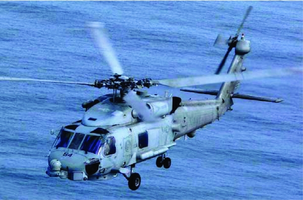
Figure 6. Sea-Hawk SH-60B helicopter.
The Flightlab model of the SH-60B comprises the following major subsystem components:
-
(1) blade-element main-rotor model including look-up tables of non-linear lift, drag and pitching moment coefficients stored as functions of incidence and Mach number;
-
(2) Bailey disk tail-rotor model;
-
(3) finite-state Peters-He dynamic inflow model;
-
(4) look-up tables for the fuselage, vertical tail and stabilator aerodynamic loads;
-
(5) turbo-shaft engine model with a rotor-speed governor;
-
(6) primary mechanical flight control system and Stability Augmentation System (SAS) models including sensor and actuator dynamics; and
-
(7) landing gear model to provide deck reaction cues on touchdown.
Padfield(Reference Padfield29) describes this level of modelling as medium fidelity, capable of simulating trim and primary-axis responses faithfully. Handling qualities characteristics are also generally well predicted using this type of flight dynamics model.
The unsteady CFD airwake simulations, described briefly above, produce large quantities of time-varying data for each of the three airwake velocity components, sampled at each point on an unstructured computational mesh, at a rate of 100 Hz (full-scale). The data in this format is unsuitable for direct implementation into Flightlab. Therefore, the data was interpolated onto a structured orthogonal grid using a linear interpolation routine, and was stored in look-up tables. Furthermore, to reduce the data storage burden and allow real-time playback of the data, only every fourth time step was used (i.e. the data was down-sampled to 25 Hz). Manual checks were performed on several of the datasets to ensure that the down-sampling did not introduce errors into the airwake data; this was achieved through visual inspection of velocity time-history plots at several locations over the flight deck, and re-computation of flow statistics using the down-sampled data. With maximum turbulent frequencies around 2 Hz, down-sampling to 25 Hz provided enough temporal resolution to ensure that velocity data remained smooth.
The structured grid was designed to cover only the region around the ship where the helicopter is expected to operate during deck landings. A uniform grid spacing of 1m was selected, as this was a close match to the element spacing on the main rotor. For the airwake model to influence the flying qualities of the simulated helicopter, the airwake velocity components must be converted into forces and moments, and applied at the helicopter model's centre of gravity. To accomplish this, local airwake velocity components are applied at a number of Airload Computation Points (ACPs) distributed around the helicopter. A total of 46 ACPs were defined for the SH-60B model, as shown in Fig. 7, including one ACP at the centre of each of the ten blade elements on each of the four main rotor blades, one at the tail rotor hub, two on the vertical tail surface, one each on the port and starboard stabilators and one at the aerodynamic centre of the fuselage.
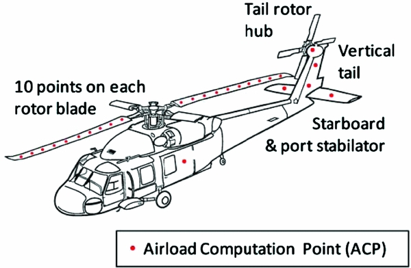
Figure 7. Location of airload computation points on the SH-60B helicopter model.
It should be noted that the interaction of the airwake with the aircraft is limited to one-way coupling. That is, the ship airwake affects the helicopter aerodynamics, but the rotor wake has no effect on the airwake (i.e. mutual ship/aircraft coupling effects are not included in the results). While it is now possible to create complete CFD calculations of a helicopter immersed in a ship's airwake(Reference Crozon, Steijl and Barakos30), for real-time piloted flight simulation the airwake is pre-computed and stored in a look-up table, and the rotor inflow model combines the airwake velocities with the induced flow.
3.3 The virtual AirDyn
The Virtual AirDyn method, which is described in more detail in Ref. Reference Kaaria, Forrest and Owen23, requires the simulated helicopter to be held fixed in space and immersed in the ship airwake while quantifying the unsteady forces and moments at the model's centre of gravity. During a simulation run, at each time step, the spatial location of every ACP is computed relative to the ship. The resulting positions in x, y and z and the time, t, are then used to extract the local airwake velocity components, at each ACP at that time, from the airwake look-up tables using a four-dimensional interpolation algorithm. The airwake velocities are defined in ship axes, so for the fuselage, empennage (stabilators and vertical tail) and tail rotor hub, these velocities must be transformed into the helicopter body-fixed reference frame. A further conversion into local rotor blade co-ordinates is required for each ACP on the main rotor blades.
During each Virtual AirDyn simulation, time histories of the unsteady forces and moments at the model's centre of gravity are recorded for 30 seconds. The data is time-averaged to enable comparisons of the ‘mean’ aerodynamic loading characteristics between each of the test points. The simulated ‘unsteady’ aerodynamic loading characteristics were generated using the method adopted by Lee and Zan(Reference Lee and Zan31,Reference Lee and Zan32) in their experimental investigations of the aerodynamic loading of a helicopter fuselage and rotor in a ship airwake. It is disturbances in the frequency range 0.2-2 Hz that have the most significant impact on helicopter handling qualities and pilot workload(Reference McRuer18). Therefore, when performing statistical analysis of unsteady loading, the usual definition of root mean square (RMS) of the deviations from the mean is not the ideal way to quantify the impact of the airwake, as it includes fluctuations at frequencies outside the bandwidth known to be responsible for airwake-induced pilot workload. Instead, Power Spectral Density (PSD) plots were derived from the force and moment time histories and the square root of the integral between the limits 0.2 Hz and 2 Hz was used as a measure of the RMS loading in this frequency bandwidth. This quantity is, therefore, referred to as the RMS loading of the particular force or moment in question (e.g. RMS yawing moment). The RMS loading in each of the 6 degrees-of-freedom has been used to characterise the unsteady aerodynamic loading of the helicopter due to the ship's airwake. It should be noted that the 0.2-2 Hz frequency range used in the current study is based on manned piloting activities with full-size helicopters; therefore, if this technique is used to evaluate airwake effects on smaller, un-manned aircraft, then this range may need to be re-evaluated.
3.4 Piloted flight simulation
While the Virtual AirDyn is able to quantify the unsteady loads imposed on the helicopter by the airwake, and thereby provide a way of comparing the effectiveness of the ship superstructure modifications, it does not directly quantify the effect of the airwake on the handling qualities of the aircraft or the pilot workload. Piloted flight trials were, therefore, conducted in the University of Liverpool's HELIFLIGHT-R flight simulator(Reference White, Perfect, Padfield, Gubbels and Berryman33). The simulator is shown in Fig. 8 and consists of an electrically actuated full motion-base platform, with the cockpit configured in a two-seat, side-by-side helicopter arrangement. Visuals are provided by three LCD projectors, giving a 220° field of view. The same SH-60B helicopter Flightlab model used for the Virtual AirDyn was used for the flight trials, with the airwake velocity components interfacing with the flight model in the same way as described previously. Computing power constraints meant that only 30 seconds of airwake could be held in the look-up tables within Flightlab (a restriction that no longer applies), so the reduced 30-second airwake was smoothly looped during the flying manoeuvres. Testing was conducted in the vicinity of a visual model of a Royal Navy Type 23 Frigate, which had been scaled such that the hangar dimensions closely matched the SFS2 geometry used to generate the airwake data; the airwake grid was then positioned such that it was correctly aligned with the superstructure. The ship forward speed was set to zero, and the ship motion was disabled to minimise additional sources of workload. Although this presents an easier challenge to the pilot, it allows the effects of the hangar modifications to be assessed in isolation.

Figure 8. The University of Liverpool's HELIFLIGHT-R flight simulator. External view (a); view from the cockpit (b).
The flight trials were flown by an ex-Royal Navy helicopter test pilot who has significant experience of ship deck landings. The use of a single test pilot was not ideal; for example, the JSHIP programme(Reference Roscoe and Thompson34) demonstrated that pilot control strategies and subjective workload ratings can vary demonstrably between different pilots. Although it was outside the scope of the current project to employ more than one test pilot, it is recognised that results from a single pilot should be approached with caution.
For each modification, the pilot was required to fly a series of Mission Task Elements (MTEs), designed to assess the impact of the modification on pilot workload. These consisted of a standard Royal Navy port-side approach and deck landing, in addition to a series of separate timed hover tasks. During the hover MTEs, the pilot was required to maintain station in a stabilised hover over the deck edge and then over the landing spot for 30 seconds each. Control activity in each of the four axes was recorded during each MTE, as was the aircraft attitude and position. A workload rating, based on the Bedford workload ratings scale shown in Fig. 9, was also reported by the pilot after each sortie.
Figure 9. The bedford workload ratings scale.
WOD speeds ranging from 30 Kn to 50 Kn were tested for each modification. To avoid needing to compute airwakes at each WOD speed, data computed at 40 Kn were scaled linearly in magnitude and frequency in accordance with Reynolds and Strouhal scaling laws. Thus, to achieve a 30 Kn wind condition, the 40 Kn velocity components were scaled down by 3/4 and the airwake playback speed was reduced by 3/4. The validity of this scaling has been confirmed by Scott et al(Reference Scott, White and Owen35).
4.0 RESULTS
As alluded to earlier in the paper, the effect of superstructure modifications on the airwake can be assessed through a CFD analysis (or wind-tunnel experiments); however, the airwake impacts upon the whole aircraft as it moves through the airwake, so an assessment of the airwake's severity from the velocity field is impracticable. The measurement of the unsteady loads obtained by the Virtual AirDyn gives information on the unsteady forces and moments imposed on the helicopter, thereby integrating the effect of the airwake on the whole aircraft, but although it provides useful information for directly comparing the ship modifications, it takes no account of how challenging the unsteady loads in the different axes are for the pilot. The results that follow will, therefore, present the effect of the hangar modifications on the airwake velocity field, on the unsteady loads imposed on the helicopter, and on the pilot workload while holding a hover position over the port-side deck edge and the landing spot.
4.1 Aerodynamic results
The first approach to assessing the impact of the geometric modifications is to analyse the statistical flow data derived from the computations. Figures 10 and 11 show contours of lateral and vertical turbulence intensity over the flight deck; these being the axes most likely to affect the tail rotor and main rotor, respectively. The turbulence intensities are with respect to the free-stream velocity. Contour plots are shown on a horizontal plane at hangar height, corresponding to the approximate vertical location of the SH-60B main rotor during the hover task, which was performed during the later flight trials. Also shown are the locations of the main rotor and tail rotor relative to the flight deck during the hover task, indicated by the black circles.

Figure 10. Contours of turbulence intensity in the lateral axis.
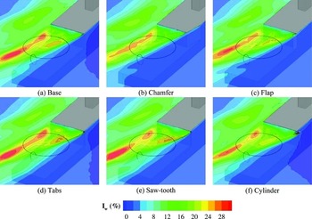
Figure 11. Contours of turbulence intensity in the vertical axis.
The flow patterns shown in Fig. 10 are similar for each of the modifications, with a significant high-turbulence region bisecting the flight deck. This lateral turbulence is associated with the flapping shear layer and is shown to cut straight through the area that would be occupied by the fuselage below the main rotor, although at this WOD angle it largely misses the tail rotor. The chamfer, flap and cylinder can all be seen to reduce lateral turbulence, with the chamfer having an appreciable reduction of up to 5% intensity over much of the flight deck. However, the tabs and saw-tooth modifications both significantly increase turbulence relative to the baseline case. A small region of high lateral turbulence can also be seen immediately aft of the cylinder, resulting from vortex shedding in its wake.
Any improvements offered by the modifications are less clear in the vertical axis (Fig. 11), although the chamfer again appears to reduce turbulence levels, particularly towards the starboard side of the flight deck. The tabs and saw-tooth are shown to increase turbulence, which is not unexpected given that they are flow spoilers. However, the turbulence contours give no information regarding the frequency content or size of the turbulent structures generated by these modifications.
Line plots showing turbulence intensity in each of the three axes are shown in Figs. 12 and 13. Data are plotted along lateral lines corresponding to the longitudinal location of the centre of the main rotor disk (Fig. 12) and tail rotor (Fig. 13) during the hover task. Spatial dimensions in the longitudinal, lateral and vertical axes are normalised by deck length l, ship beam b and hangar height h, respectively. The port side deck edge is, therefore, at y/b = −0.5, and the starboard deck edge is at y/b = 0.5.
Figure 12. Turbulence intensity along a lateral line aligned with the landing spot at hangar height (located at x/l = 0.55 and z/h = 1). Longitudinal (a), lateral (b) and vertical (c) intensities plotted, normalised by free-stream velocity.
Figure 13. Turbulence intensity along a lateral line coincident with the location of the tail rotor during hover (located at x/l = 0.9 and z/h = 1). Longitudinal (a), lateral (b) and vertical (c) intensities plotted, normalised by free-stream velocity.
In all axes, the chamfer and flap are shown to deflect the shear layer towards the port side, leading to a reduction in turbulence over the starboard side and a corresponding increase to port compared with the other geometries. However, the overall effect is a total reduction in turbulence at both longitudinal locations for these modifications. The cylinder can be seen to reduce both the peak magnitude and width of the main turbulent region, particularly in the lateral and vertical axes, although improvements are limited to a few percent compared to the baseline case. Again, the tabs and saw-tooth modifications are shown to increase peak turbulence levels over much of the flight deck.
It is clear from the analysis above that several of the modifications lead to significant differences in the turbulence field of the SFS2 airwake. For example, over the landing spot lateral turbulence intensity for the tabs and saw-tooth is approximately 45% higher than for the chamfer (Fig. 12(b)). However, it is still unclear what level of turbulence reduction is required to make a tangible difference to the difficulty of deck landings.
4.2 Virtual AirDyn results
The helicopter model was placed at a total of 35 points over the flight deck, with the aircraft positioned such that the main rotor was at the same height as the top of the hangar (a typical height during a landing manoeuvre). Figure 14 shows the test matrix, with each node on the grid corresponding to a sampling location where the rotor hub was positioned. Before sampling began, the helicopter model was trimmed in free-stream conditions (Green 30° at 40 Kn) to minimise the effects of differential lift across the disk; the control positions were then fixed for the duration of the run. Each of the helicopter's linear and rotational degrees of freedom were then disabled, to ensure that the aircraft remained fixed at the sampling position. All forces and moments on the helicopter model were recorded during each 30 second sampling period; these time histories were then used to calculate the RMS loading on the aircraft due to the airwake as described above. As explained by Kaaria et al(Reference Kaaria, Forrest and Owen23), it is the mean aerodynamic loads that are largely responsible for eroding the helicopter's control margins, and the unsteady components that are largely responsible for pilot workload.
Figure 14. Grid showing helicopter model locations during virtual AirDyn testing. AirDyn sample locations are denoted by black dots; location of the landing spot is indicated by the black circle.
Figures 15-20 show contours of RMS loading in the helicopter's force and moment axes for each of the modifications tested. Some marked differences between modifications can be observed, both in terms of the location and magnitude of unsteady loading. Most of the trends seen in the CFD results are detected by the helicopter model; that is, modifications giving rise to high levels of turbulence lead to high RMS loading values, and vice versa. However, the Virtual AirDyn provides more valuable information than point turbulence values, as it takes into account the effects of the airwake over the whole aircraft. Furthermore, there is no need to decouple the three components of turbulence and assess their impact separately, as is common in ship airwake studies, which focus purely on the aerodynamics. In using a fixed helicopter model to assess the airwake, the effects of all three velocity components are implicit in the RMS loading results, which are quantities that can be directly related to the aircraft control axes and, therefore, pilot workload.

Figure 15. Contours of RMS loading in the aircraft longitudinal axis for the various modifications.

Figure 16. Contours of RMS loading in the aircraft lateral axis for the various modifications.

Figure 17. Contours of RMS loading in the aircraft lift axis for the various modifications.

Figure 18. Contours of RMS loading in the aircraft roll axis for the various modifications.

Figure 19. Contours of RMS loading in the aircraft pitch axis for the various modifications.

Figure 20. Contours of RMS loading in the aircraft yaw axis for the various modifications.
As would be expected, the largest force RMS loading values are seen in the aircraft's lift axis, parallel to the main rotor's thrust vector (note the different scales on each figure). In terms of moment RMS loading, yaw is dominant, followed by pitch, then roll. However, the relative magnitude of loading in these axes is shown to vary over the flight deck. This is consistent with pilot comments from the simulation flight trials, which indicated that airwake disturbances are multi-axis, requiring consistent correction in all flight controls.
It is clear from each of the figures that the chamfer and flap lead to larger regions of undisturbed free-stream flow over the flight deck, indicated by the dark blue shading. This port-side deflection of the separating shear layer was also seen in the CFD results. In fact, all of the features seen in Figs. 15-20 can be directly related to the airwake topology. For example, Fig. 20 shows that, for most modifications, RMS loading in yaw is greatest when the helicopter is located at the front of the grid, at a lateral location around y/b = −0.4. From Fig. 10, it can be seen that at this location the tail rotor is in the area of highest lateral turbulence. Similarly, the lift axis is most active in the aft region of the sampling grid, towards the port side (Fig. 17). This coincides with the region of high vertical turbulence intensity at the aft/port area of the flight deck as seen in Fig. 11.
As an overview of the results shown in Figs. 15-20, the greatest improvements relative to the baseline case are given by the chamfer, followed by the flap. The cylinder improves the flow in some areas, while worsening it in others. Finally, the tabs and saw-tooth both significantly increase unsteady loading in most axes.
Quantifying the improvements offered by the chamfer over the base SFS2; the biggest reductions in RMS loading are seen in yaw (45%), followed by roll (30%), then lift (25%). However, it should be noted that these improvements are not necessarily directly over the landing spot. Indeed, the highest loading values can generally be seen over the port-side deck edge, which is where the chamfer and flap show some of the greatest improvements.
4.3 Flight test results
Figure 21 shows workload ratings for the landing spot and deck edge hover tasks as reported by the pilot. Best-fit straight lines have been included to indicate the general trends, although it is recognised that these are based on limited datasets. More data are available for the landing spot hover task, as during the flight testing it was possible to repeat these MTEs several times; however, an appreciable amount of scatter is still seen.
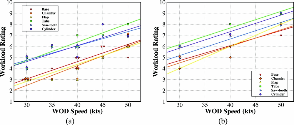
Figure 21. Bedford workload ratings given for a 30-second hover over the landing spot (a) and port-side deck edge (b).
The first thing to notice from both plots is the consistent increase in workload rating with increasing WOD speed. This is to be expected due to larger magnitude gusts requiring a higher gain control strategy to counteract. It can also be seen that workload ratings over the deck edge (Fig. 21(b)) are, on average, one to two points higher than over the landing spot (Fig. 21(a)). This corresponds well with the results from the Virtual AirDyn, where the highest RMS loading values were observed over the port-side deck edge.
In terms of the effectiveness of the modifications, they appear to be grouped into a lower band consisting of base, chamfer and flap; and an upper band consisting of the cylinder, tabs and saw-tooth. This indicates that the modifications that were previously shown to increase turbulence and RMS loading also lead to an increase in reported pilot workload. However, the chamfer and flap that were shown by the Virtual AirDyn to reduce the severity of the airwake do not give rise to significantly different results from the un-modified SFS2.
Differences between the improved airwakes and the baseline case can be detected in analysis of the pilot control activity. Figure 22 shows power spectral density plots of the normalised cyclic and pedal inputs during the landing spot hover task for the 40 Kn WOD condition. It should be noted that during data analysis it was discovered that a portion of the pedal input time history from the tabs run was corrupted, so it has been omitted from the plot in Fig. 22.
Figure 22. Power spectral density of pilot control activity during a 30-second hover over the landing spot. (Note: the ‘tabs’ data is not shown in the pedal chart due to corruption in the pedal data stream during recording.)
The longitudinal cyclic axis, corresponding mainly to disturbances in pitch, sees approximately twice as much activity as the lateral, or roll, axis. This agrees well with results from the Virtual AirDyn, which showed that RMS loading in roll was, on average, half that in pitch (Figs. 18 and 19). In both cyclic axes, the highest peaks in the PSD plots are from the saw-tooth and tabs modifications, closely followed by the cylinder.
Compared to the base case, the cylinder plot extends to higher frequencies for all control axes and sees a slight reduction in PSD at the lower end of the spectrum. This may be due to the introduction of higher frequency turbulence by the vortex shedding from the cylinder, although this does not appear to have the desired effect of reducing workload in the pilot's closed-loop control bandwidth.
The chamfer results in reduced PSD values compared to the base geometry in all control axes, particularly in the range 0.4-1 Hz. This is also seen for the flap modification, except in the lateral cyclic axis, where a large peak is seen at 0.5 Hz.
It is unclear why the reduced control activity for the chamfer and flap shown in Fig. 22 does not result in lower workload ratings from the test pilot. However, it is encouraging that modifications shown by the Virtual AirDyn to worsen the flow are seen to produce a corresponding increase in pilot workload during the flight tests.
Although some of the modifications tested were shown to lead to improvements in airflow over the flight deck, it should be reiterated that testing has so far only been carried out for a single Green 30° WOD condition. It is quite possible that modifications that improve the flow at one WOD condition may make things worse at another, and vice versa. Similarly, the modifications presented here have not undergone any kind of optimisation in terms of size, orientation or placement. There is, therefore, significant scope for future studies in this area.
5.0 CONCLUSIONS
The main purpose of this paper has been to demonstrate how ship design modifications can affect the ship airwake and the subsequent handling qualities of a helicopter operating over and around the landing deck. The effectiveness of a selected number of hangar-edge modifications have been assessed using flight mechanics modelling (Virtual AirDyn) and piloted flight simulation. The real benefit of these tools is that they can be used during the ship design process to evaluate the effect of the superstructure aerodynamics, rather than wait until after the ship is built. To illustrate how CFD, the Virtual AirDyn and piloted simulation can contribute to understanding how the ship geometry will affect the helicopter, the paper has presented results from modifying the windward vertical rear edge of the hangar in an oblique wind. Such modifications, as has been demonstrated, will mainly affect the flow interacting with the tail rotor and the fuselage and will impact less on the main rotor. It should also be borne in mind that the modifications have only been evaluated for one wind angle whereas in reality improvements will be required for all wind angles. Clearly, to evaluate a ship superstructure for all wind angles and with different geometries is a major study beyond the scope of a technical paper. However, the results in this paper have demonstrated how the simulation techniques can be applied.
For the limited conditions explored in this paper, the following conclusions can be drawn:
-
• Modifications to the edges of a ship's superstructure can be used to affect the airwake and hence the aerodynamic loading on a maritime helicopter operating over and around the landing deck of a ship.
-
• The Virtual AirDyn is an effective and versatile tool for evaluating and comparing different ship designs. It can be used to identify promising geometric configurations, and then the more elaborate and time-consuming piloted simulations can be used to assess the effects of the selected geometries on the aircraft handing qualities and pilot workload.
-
• The vertical hangar-edge modifications which guide the flow around the hangar edge, chamfer and flap, produced a reduction in airwake turbulence over the flight deck and a corresponding decrease in unsteady loads and pilot workload.
-
• The vertical-edge modifications that were intended to break up the separated flow – tabs, sawtooth and cylinder – generally led to an increase in turbulence, unsteady loading and pilot workload.
ACKNOWLEDGEMENTS
The authors would like to thank the test pilot, Andy Berryman, for his professionalism and guidance. Many hours of help and support have also been given by Philip Perfect, Neil Cameron and Mark White from the University of Liverpool's Flight Science and Technology research group. Cliff Addison helped immensely with the computing cluster set-up and maintenance. The ongoing support given by ANSYS Inc to this research is also gratefully acknowledged.


