


1. Introduction
Optimal flight trajectories have been of interest since the beginnings of aviation, but the subject has gained more attention recently, for the following reasons:
• free route airspace replacing the classical airways network creates unprecedented opportunities for optimal trajectory solutions;
• greener aviation policies push for the implementation of optimal flight trajectories more than the cost of fuel previously did;
• advancements in air to ground data link and the connection between flight management computers and electronic flight bag applications, making use of the weather forecast and enabling trajectory optimisations.
Another circumstance which stimulates the study of the optimised flight trajectories is the development of the electrical propulsion, especially in the unmanned aerial system (UAS). The use of low energy density sources increases the demand for optimal navigation, and the low airspeed performance of unmanned vehicles such as multi-copters make their flight even more sensitive to wind.
Flight trajectory optimisation problems are tasks in search of the following:
• the best use of the atmosphere as a moving layer (due to wind), based on the weather forecast;
• the best use of the aircraft aerodynamics and engines;
• the best use of the airspace capacity, considering other traffic and the air traffic management constraints;
• the minimisation of risks (safest solution).
The latter criteria gained visibility and importance in the air traffic management (ATM) context, because in a crowded airspace, it is less relevant to optimise a single trajectory, as if other traffic were not present. The optimal trajectory results from considering the traffic situation and all ATM constraints (Pleter, Reference Pleter2004; Pleter et al., Reference Pleter, Constantinescu and Ştefănescu2006, Reference Pleter, Constantinescu and Ştefănescu2009; Gardi et al., Reference Gardi, Sabatini and Ramasamy2016).
Air navigation problems are particularly sensitive to the wind forecast, because the wind has a significant and direct impact on the flight. The modern jet airliners cruise at heights where the winds are usually strong and permanent, frequently over 50 kts but possibly up to 200 kts, which represents 40% of the usual true airspeed (TAS) of the aircraft at that altitude. Even the surface winds may account for a large proportion of the airspeeds of small aircraft, such as quadcopters. The atmosphere carries in the motion any atmospheric flying object. The wind carries the airplane, regardless of its weight, in equilibrium flight conditions. A 500 tonnes Airbus A380 is equally impacted by the wind as a quadcopter of half a kilogram in equilibrium flight. Non-equilibrium flight or ballistic flight is possible for very short periods (for instance when the wind changes) but the total time of such periods is negligible as compared to the total flight time. The overall effects of such transitory phenomena are negligible in amplitude, time and they cancel each other (out of randomness).
Terrestrial vehicles, including aircraft rolling on the ground, cancel crosswind by the reaction friction force between the wheels and the ground. Even in maritime navigation, boats and ships are protected from the impact of the wind by the hydrodynamics at the contact of the ship with the water. Most of the effect of the wind is cancelled by friction. During the take-off roll of an airplane in crosswind, the pilots need to apply small steering corrections from time to time, like in a car. At the moment of lift-off, the friction force between the landing gear wheels and the runway disappears, and suddenly the airplane is carried by the wind fully (Figure 1, left). Figure 1 captures this rapid change of trajectory at lift-off (it is not sudden due to inertia of the airplane, but it is fast).

Figure 1. Wind influence on an aircraft moving on the ground during take-off run (left) and airborne (right). The variables are explained in Table 1. The ground speed GS is tangent to the trajectory TRK everywhere except at lift-off, where there is a fast change of the track azimuth
Table 1. Abbreviations of the variables in Figure 1

Optimal flight trajectories should first take advantage of the wind, changing shape as to maximise the tailwind integral and to minimise the headwind integral over the duration of the flight. This is the brachistochrone concept presented later. Second, optimal flight trajectories should attempt to achieve the best use of aircraft aerodynamics and engines (aircraft performance, Camiller et al., Reference Camiller, Chircop, Zammit-Mangion, Sabatini and Sethi2012). The Bréguet differential equation (Bovet, Reference Bovet2019) formalises the concept and indicates that the best aerodynamics is related to the best lift-to-drag ratio (L/D) at a certain weight of the aircraft, but the weight is continuously decreasing due to the burning of fuel. Also, the best L/D would extend the duration of the flight due to the low Mach number. In practice, the optimality of the airliner navigation is a trade-off between fuel savings and performance (true airspeed), taking the cost index (CI) preferred by the airline as a parameter, as the input into the flight management system (FMS). At the lower end of the airspeed envelope, the aircraft develops the maximum L/D and has the maximum range with a given amount of fuel at departure, but this on the edge setting is not acceptable due to safety reasons. At the higher end of the airspeed envelope (of the Mach number, because the maximum operating Mach (MMO) is what limits an airliner at cruise level to fly faster), the duration of the flight is minimum, but the compressibility drag increases nonlinearly and the fuel burn increases considerably due the shock wave formation. The increase in performance is traded off by a parabolic increase in fuel burn with its subsequent range cut, which must stay above the distance planned (with the required reserves). The CI is used to quantify the fuel economy in the trajectory optimisation, as a trade-off parameter input into the FMS before the flight (Bulfer and Gifford, Reference Bulfer and Gifford1999). Since its introduction in the 1980s by Boeing, this parameter was constant all along the flight, but modern approaches towards flight trajectory optimisation demand possible updates along the flight. Figure 2 illustrates the total fuel burn for a certain flight as a function of CI. For each CI, there is a corresponding target Mach number, which the FMS will try to achieve via the automated flight control system.
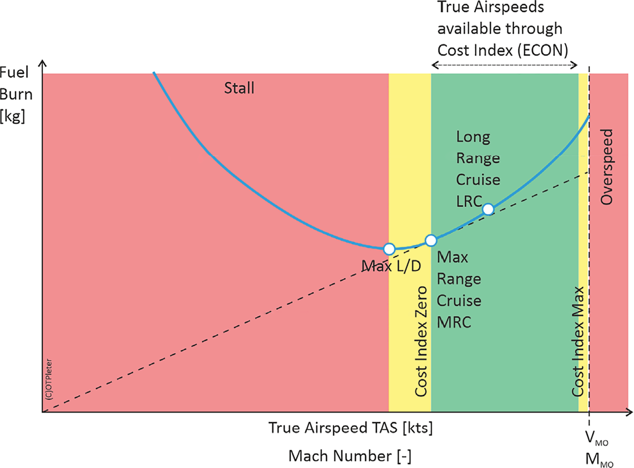
Figure 2. Cost index (CI) setting and its influence on the true airspeed, Mach and fuel burn. This is a generic diagram. Numerical values would require a specific aircraft type, mass and flight level
Apparently, the brachistochrone problem and the aircraft performance problem do not overlap, since the first only concerns the Earth atmosphere and the second only concerns the aircraft and eventually its engines. In reality, the two problems are coupled on two counts:
• the wind vector field is continuously changing, so a different target airspeed will make the aircraft experience a different wind situation along the way;
• the aircraft performance is exclusively measured in an atmospheric frame, whereas reaching a destination is referenced to the ground, so the wind intervenes anyway, and ultimately, the ground speed rather than the airspeed is what matters in navigation.
The brachistochrone is believed to become more relevant in the ATM environment, with the implementation of the free route and with the increasing demand for greener flights. Currently, the flight trajectory efficiency is still measured by comparing real flights with the orthodromes (EUROCONTROL, 2020). Consequently, all optimised trajectories calculated by the specialised software airlines have been using for some time (Emirates, Qantas, British Airways, Lufthansa etc.) and the brachistochrones in the case studies below would be considered ‘inefficient’ by current ATM metrics, since they diverge from the great circle routes. This prompts for a reconsideration of the flight efficiency standards and metrics.
2. The Wind Triangle
Figure 3 illustrates the wind triangle in three dimensions. The aircraft develops a certain speed relative to the surrounding atmosphere (true airspeed or TAS), and the atmosphere moves with respect to the ground with the wind velocity (WV), which may be decomposed into three components: u, v and w. For navigation, the Earth speed (ES) relative to the ground is the result of the vector addition between TAS and WV. In the vertical projection, ES is decomposed into the ground speed (GS) horizontally and the vertical speed (VS*) vertically. GS is particularly relevant to navigation, because it generates the horizontal projection of the flight trajectory and marks the progress of the aircraft along the track to the destination. In a horizontal plane, the GS is the result of a vector addition of the true airspeed of the aircraft (TAS) flying level and the local WV, given by u and v components.

Figure 3. Speed triangle in vertical and horizontal navigation
Horizontal wind triangle problems are essentially two functions of two variables, the impact angle ζ (the angle made by the wind direction and the flown track) and the velocity ratio ξ (the ratio between the wind velocity and TAS). The two functions are DA (drift angle) and GT = GS/TAS (the GS-to-TAS ratio), represented as surfaces in Figures 4 and 5. All brachistochrone optimisations will use these surfaces to locally define navigation, to be integrated for the entire flight. Optimisation consists of searching for the shortest time of flight trajectory out of all or at least many of the possible variants. The cross-section curves allow a graphical insight into the problem, locally. A tangent plane frame with two orthogonal axes true north (TN) and true east (TE) serves well the horizontal navigation except for the polar regions, where, due to the fast convergence of the meridians, the axes should be arbitrary grid axes. The dead reckoning equations define the horizontal projection of the flight trajectory and the progress along the route (Kayton and Fried, Reference Kayton and Fried1997):


Figure 4. Drift angle (DA) surface as a function of ζ and ξ. The DA uses a sign convention: + for right (clockwise) and − for left

Figure 5. GS-to-TAS ratio (GT) surface represented as a function of ζ and ξ
The horizontal wind is dominant (in comparison, the vertical wind is negligible at the scale of an airliner flight route) and there are three variants of representing it:
• the wind direction from which it blows, in degrees from true north, followed by the ‘/’ symbol, followed by the wind velocity in knots – WD/WV (for surface wind communicated by radio by Air Traffic Control (ATC), magnetic north is used), which is the usual expression of the wind in ATC and aeronautical information systems (METAR, VOLMET etc.);
• u and v components, where the zonal velocity u, the component of the horizontal wind towards true east, and the meridional velocity v, the component of the horizontal wind towards true north, are the usual expression of the wind in the meteorological databases, using the standard GRIB format;
• headwind, tailwind and crosswind components, which are the horizontal components of the wind with respect of the aircraft, where the headwind and tailwind are the longitudinal axis components and the crosswind is along the lateral axis. The headwind component blows from the front of the aircraft, slowing it down, and the tailwind component blows from the back, speeding up the aircraft with respect to ground. Pilots prefer this format, since they can immediately see the impact on navigation, and also make decisions on matters like tailwind landing limitation or crosswind landing limitation.
The wind triangle equations are


where γ is the trajectory path (Figure 3). In cruise flight, γ = 0. With the components, we may calculate the vector module and direction:


In the applications presented in this paper, we will solve the direct wind triangle problem (GS and TC unknowns) by using the u and v wind components:

This system may be converted to a second-degree equation by squaring each equation and adding them together:


The roots of the resulting equation are

where $c \equiv \cos ({TC} )\cdot v$ and $s \equiv \sin ({TC} )\cdot u$
 . The negative root is false.
The horizontal navigation equations can also be written in a differential form, to be integrated with respect to time. For longer flights, we may upgrade from a local tangent plane reference system to geodetic spherical coordinates (GSC) for instance and work with the WGS84 rotation ellipsoid curvature:


where H is the height of flight above sea level, and the curvatures of the WGS84 ellipsoid are taken from ICAO (2002).
3. Brachistochrone
The word brachistochrone is coined from mechanics, where it originated with the meaning of the shape of a slide which ensures that a free sliding body under the influence of gravity only arrives at the bottom in the shortest amount of time. This classic problem was formulated and solved by Johann Bernoulli in 1696. He used the Greek words brákhistos khrónos (short time). Here the word is used in the sense of the shortest time air navigation trajectory. In maritime navigation, the shortest route (the orthodrome or the great circle route) is the preferred navigation route. In air navigation that is not the case, because of the major impact of the wind. Aircraft fly with respect to the atmosphere, and the wind represents the velocity of the atmosphere with respect to the ground. The resultant velocity is affected by the slightest wind, and under the equilibrium flight conditions (which could be assumed for airliners flight for the quasi-totality of the flight duration), any aircraft is equally affected, irrespective of its mass. In the absence of wind, the brachistochrone is an orthodrome. The brachistochrone is also identical to the orthodrome when the wind vector field has zero divergence and curl. However, the typical wind vector field is naturally rich in divergence and curl, and large wind rotors are often encountered. The use of the term brachistochrone in air navigation must be taken as a proposal in this paper, because it is not widely accepted. The more frequently used equivalent is the minimum time trajectory, but this is long and invites a possible confusion mentioned later.
The concept of brachistochrone aims at the minimum time of flight for a given TAS (consequently Mach number), but not the absolute minimum, because this would imply maximum TAS. In this case, the compressibility drag, which grows parabolically with the airspeed, will cancel the fuel savings by the large thrust required from the engines. Such a very fast flight would end up with more fuel consumption than any of the slower variants of the trajectory, despite the faster time of flight. We take the brachistochrone from the atmosphere movement point of view, as the minimum time of flight of an aircraft cruising at a given TAS. Of course, the brachistochrone changes if the TAS changes, because the wind vector field is a function of time. As compared to the orthodrome, which may be calculated using spherical trigonometry, the brachistochrone requires the wind vector field forecast in space and time. The forecast should cover the whole region between the departure and the arrival aerodromes, and should cover the entire duration of the flight. Normally the weather forecast is available in GRIB format at certain times T: T + 0 h (nowcast), T + 3, T + 6 etc. The points where the wind direction and velocity are specified correspond to a grid with a certain step (e.g., 10 NM), covering the entire planet. These data should be sufficient to estimate the wind along the flight, by bi-linear or bi-spline interpolation in space and by linear or spline interpolation in time.
The problem with the brachistochrone is that it depends on the wind forecast, so there is a different solution every time we perform a calculation. Also, the solution may not be efficient if the weather forecast is not accurate, which means that the brachistochrone is to be calculated as late as possible before the flight, to ensure the most accurate forecast.
As a definition, the brachistochrone is the optimal flight trajectory in the atmosphere on the sphere or on the ellipsoid, considering the wind velocity (maximising the tail wind and minimising the head wind over the duration of the flight). The forecasted wind vector field in the larger flight area over the duration of the flight is required. The brachistochrone is independent of the flight performance optimisation (range versus speed), as computed by the FMS. Whichever CI is selected, the brachistochrone is the best flight trajectory at that target Mach number which results from the CI, and it is best as per the minimum time of flight. Obviously, the absolute minimum time of flight would be achieved with the maximum CI input, i.e., maximum operating Mach number MMO. Usually, this takes the maximum fuel burn, due to the nonlinear steep increase of the compressibility drag as the Mach number approaches the sonic barrier. Therefore, the absolute minimum time of flight is the least cost efficient solution: burns more fuel and consequently produces more emissions. The fuel flow is so much higher that even though the flight duration is shorter, the total fuel burn is the highest. However, as mentioned before, the brachistochrone does not regard that absolute minimum time, it concerns just the wind vector field. How fast is the aircraft flying with respect to the atmosphere is a separate matter. All these qualify the brachistochrone as the greenest trajectory solution, the most fuel and emissions efficient solution relative to the atmosphere.
The brachistochrone problems may be classified, as in Table 2. Solving these problems can be done directly in Matlab, which may also import and use the meteorological GRIB files (NOAA, 2021). In Section 4, the brachistochrone problem will be generalised to find the optimal trajectory.
Table 2. Classification of brachistochrones

The brachistochrone problem may also be solved by multimodal optimisation: we take a large sample of weather situations and cluster resulting brachistochrones. For each individual weather forecast, the brachistochrone belongs to a certain cluster, and the cluster prototype may be used as a flight plan.
Not even the simplest artificial case of the 2D brachistochrone problem admits an analytical solution. The following numerical examples were calculated using genetic algorithms in Matlab.
4. Brachistochrone case studies
The following cases were selected on relevance, with flight duration of approximately three hours in a typical jet airliner over the Black Sea. The area was chosen for the larger typical divergence and vorticity of the wind vector field, and also a variety of wind directions at different isobaric layers. There are certain situations in the Black Sea area (for instance, on 11 November 2018), when the wind is blowing from different directions at different flight levels, covering all four cardinal directions at the same time (NOAA, 2021). However, similar results are expected from longer flights, in any other parts of the world. The flight departure and arrival airports which were selected for these examples are presented in Table 3. The choice of these airports was made for their location, diametrically opposed with respect to the Black Sea.
Table 3. Case studies departure and arrival airports

Enroute optimisations, as presented below, assume the whole trajectory is at the cruise level, ignoring the phases of climb and descent. For long range flights, this assumption is fair, for two reasons: (1) climb and descent combined take less than one hour of flight time; (2) cruise flight fuel flow is an average of the climb and descent fuel flows, so the error made during the climb phase is offset by the error at descent (a small margin remains though, caused by the idle thrust fuel flow, the fuel required just to keep engines in motion during descent).
4.1 2D brachistochrone
This case study uses a single simulated wind vortex over the Black Sea for a flight from Athens to Samara, at a typical flight level FL390 (39,000 ft isobaric surface), with a constant Mach number M0⋅78 in international standard atmosphere (ISA) conditions (TAS = 447 kts, calibrated airspeed CAS = 240⋅8 kts, total air temperature TAT = −30⋅18 °C, outside air temperature OAT = −56⋅5 °C, static pressure ps = 196⋅8 hPa), (ICAO, 1993).
The simulated wind vector field is based on a counter-clockwise wind rotor simulated over the Black Sea, with a maximum wind velocity of 90 kts at the vortex radius of approximately 240 NM. Wind velocity distribution inside this circle is decreasing to zero linearly, whereas outside it is decreasing slower (inverse parabolic), as to make a plausible artificial case (Figure 6).

Figure 6. Counter-clockwise wind vector field rotor simulated at the midpoint of the orthodrome between LGAV and UWWW (dashed line). The brachistochrone is represented as solid line.
The centre of the rotor is placed in the orthodrome midpoint: N46°28′E035°11′.
The orthodrome (or great circle) distance is 1428 NM at the sea level and 1430 NM at the height of the flight (FL390), using a spherical approximation of the Earth. Matlab distance function using WGS84 indicates 1426⋅8 NM at the sea level, which could translate into 1429 NM at the cruise level. In absence of wind, at M0⋅78 the distance is covered in estimated time enroute ETE = 11,517 s (3 h 11 min 57 s). The loxodrome (rumble line) distance is 1437 NM.
For the brachistochrone optimisation in Matlab, a granularity of N = 12 equally spaced waypoints WPTk was used, with departure (D) and arrival (A) fixed, and with 10 movable intermediary waypoints. The optimisation algorithm searches where to move these intermediary waypoints along the meridian (left or right of the track), to minimise the time of flight, taking advantage of the wind. This corresponds to N − 2 = 10 multiplied by two (LAT and LONG) = 20 degrees of freedom of the optimisation problem. Also, to increase accuracy, a number of intermediary points were needed to solve the wind triangle problem on each leg between two successive waypoints. In this case, the wind triangle problem was solved at every waypoint and additionally at a number of M = 3 equally spaced intermediary points of each leg. Without these intermediary points, the errors become noticeable at N = 12. However, increasing N itself is less desirable, since it impacts the running time.
The optimisation in Matlab used genetic algorithms and took almost 700 generations to get to the results in Figure 7.

Figure 7. 2D brachistochrone calculated in Matlab. The fitness index based on the time of flight ETE is minimised to 11,319.2 s (above). The deviations from the orthodrome in degrees of latitude (1° is approximately 60 NM) are represented below for the N − 2 = 10 intermediary waypoints
Table 4 presents the 2D brachistochrone optimisation results. The distance increased to DIS = 1482⋅5 NM, but the time decreased to ETE = 11,319 s = 3 h 8 min 39 s.
Table 4. 2D brachistochrone case study results

The time gain of 350 s or 5 min and 50 s may not seem a lot, but the fuel gain for a typical twin-engine airliner could be 800 kg of fuel for this flight. For this single rotor case, the brachistochrone deviates from the centre, leaving the wind to drift the airplane away in the first part of the flight, up to the rotor centre, and then leaving the wind to bring it back to the destination in the second part. Such a shape was expected and may be explained intuitively: instead of fighting the left crosswind component in the first half of the flight and the right cross wind component in the second half, just for the sake of keeping the desired track, the flight is better off by letting the wind do its work to a certain extent.
The process was repeated with the same data for six distinct airspeeds, and the results are presented in Table 5. As in the basic wind triangle problem, what is relevant is not the absolute value of TAS, but the wind velocity to TAS ratio, named ξ. The wind velocity is variable in this case, but it is limited at 90 kts, so the ξ max can be calculated.
Table 5. 2D brachistochrone case study results

The relative difference between the brachistochrone and the orthodrome is presented in column ΔETE and ΔDIS. An almost perfect correlation can be noticed between the relative differences and the ξ max column. The faster the airplane with respect to the wind, the less time can be saved by the brachistochrone, and the smaller the diversion which extends the distance.
4.2 3D brachistochrone
The weather in the next case is real and it was taken from NOAA as of the 5th of August, 2021 18:00 UTC (NOAA, 2021). The flight level is an additional dimension with the corresponding degrees of freedom represented by FLk (flight level in each waypoint k). The airplane is free to climb and descend along the route to minimise the time of flight. The selectable flight levels were compliant with the reduced vertical separation minima (RVSM) scheme, so just the odd levels (FL290, FL310, FL330, FL350, FL370, FL390 and FL410) were considered for this Eastbound flight. The flight levels above FL410 were not included in the search due to flight performance limitations of the aircraft considered in this example. The levels below FL290 are not suitable for cruising for a turbofan engine powered aircraft. In a theoretical optimisation case, the optimal flight level could be found on each leg by the 3D brachistochrone algorithm. In this example, more realism was added by selecting the nearest RVSM compliant level from the above list. Cruising on intermediary levels is currently not acceptable for the ATM system, because a single flight would occupy two slots simultaneously, penalising capacity. Perhaps this restriction will be removed in a future automated trajectory-based ATM system, and that would add more potential to the 3D brachistochrone optimisation (Figure 8).

Figure 8. 3D brachistochrone calculated in Matlab. The fitness index based on the time of flight ETE is minimised to 12,103 s (above). Below, the 20 variables are split in two sections: the deviations from the orthodrome in degrees of latitude, and the flight level FL, each for the N − 2 = 10 intermediary waypoints
Input data for this numerical case are the following: M0⋅7 TAS 400 kts, starting flight at FL390 but allow its change in any of the N − 2 = 10 intermediary waypoints. After close to 800 generations, the genetic algorithm converged to a solution with ETE = 12,103 s (3 h 21 min 43 s), saving 183 s of flight time from the orthodrome flight. The route is Northern as expected, since the rotor is clockwise, in contrast to the previous examples. The FL is FL410 in the first part of the flight, with the exception of the first leg, where the initial FL390 was forcefully used by the algorithm. In the second part of the flight, the optimiser sensed a benefit from descending to FL390, and later to FL350, contrary to the classic step climb strategy (Figure 9).

Figure 9. 3D brachistochrone calculated in Matlab with the wind vector field at FL410
The next levels of brachistochrones, as presented in Table 2, are enhancements of the algorithm as follows:
• 3D BRACHISTOCHRONE WITH FLEXIBLE TIME OF DEPARTURE – the optimisation variable which is introduced in this case, in addition to the 3D brachistochrone, is a time delay in the estimated time of departure (ETD). The algorithm would again try to minimise the time of flight, but depending on the ETD, the wind situation along the way changes, and one 3D brachistochrone would hopefully stand out as the best one. The rationale of this category is the possibility that a flight could delay departure to benefit from a temporary better wind. A delay in the ETD has to be allowed anyway in flight trajectory optimisation problems due to the flight capacity constraints. When somewhere along the route the air traffic management capacity is exceeded, that flight needs to delay its departure due to traffic. The delay in the ETD plus the time of flight cannot exceed the scheduled estimated time of arrival (ETA), but this is very conservative, based on the worst case of wind configuration.
• 4D BRACHISTOCHRONE is similar to the previous one, but instead of delaying the departure to access a better wind situation, the Mach number (and consequently the airspeed) is changed and considered an additional optimisation variable. This new variability is used to achieve the best 3D brachistochrone. The Mach number must be sought in the speed range, according to the FMS (between MRC and MMO, see Figure 2).
• 4D BRACHISTOCHRONE WITH FLEXIBLE TIME OF DEPARTURE is the concept of brachistochrone pushed to its limit, considering simultaneously a variable ETD and a variable M along the flight.
5. Multidisciplinary optimisation
The optimal flight trajectory results from a multidisciplinary optimisation, using the total costs and risks (TCR) as the objective function to be minimised. Experimental results are given in previous work (Pleter, Reference Pleter2004; Pleter et al., Reference Pleter, Constantinescu and Ştefănescu2006, Reference Pleter, Constantinescu and Ştefănescu2009). As optimisations perform better when the scope is extended, the best scope is the entire gate-to-gate flight (G2G). If the optimisation is run at a time when a flight has already departed, the scope of the optimisation evidently runs just for the remaining portion of the flight, from the current moment to the arrival gate (parking position). Among other factors, it should consider integrating over the entire duration of the flight the following:
Cost factors:
• fuel cost Cf;
• navigation cost Cn (ATS – Air Traffic Service charges, eventual costs of slots or of the opportunity to use the air navigation infrastructure at a time of peak demand);
• maintenance cost Cm (time based and structural load / propulsion system load based);
• depreciation of the aircraft Ca (amortisation per hour of flight, time based);
• cost of delays Cd (commercial costs due to significant delays);
• cost of airspace capacity Cc (for instance, flight between established flight levels, very slow climb, very slow descent);
• environmental cost Ce (including noise emissions, CO2, NOx, soot, contrails);
• cost of navigation optimisation Co (the cost of solving the optimisation problem itself, based on the granularity and the complexity of the models involved).
Risk factors:
• weather risk Rwt, Rwi (turbulence, icing);
• wake vortex risk Rwt (turbulence created by proximate traffic);
• loss of separation risk Rls (vertical and horizontal separation);
• terrain proximity risk Rtp (obstacle clearance);
• low fuel risk Rlf (arrival priority based on remaining fuel on board);
• depressurisation risk Rd (flying over Himalayans or other wide mountainous areas);
• emergency risk Re (flying far from suitable airports for eventual emergency landing);
• manoeuvre hazard Rm (flying within the range of unexpected manoeuvres by proximate traffic);
• protected airspace intrusion risk Rp (no fly zones, prohibited areas PA, restricted areas RA, danger areas DA);
• security risk Rse (flying in hostile areas or conflict zones);
• safety risk Rsa (flying in areas with lower safety standards).
Most of these factors were presented, explained and quantified by Pleter et al. (Reference Pleter, Constantinescu and Ştefănescu2006, Reference Pleter, Constantinescu and Ştefănescu2009) or by Camiller et al. (Reference Camiller, Chircop, Zammit-Mangion, Sabatini and Sethi2012). Risks might be expressed as costs by multiplying the possible damage with the probability of the unwanted outcome. This allows the addition of the risks with the costs in computing the TCR index. The probability of an unwanted outcome over the entire duration of the flight could be calculated as integrating a hazard function, based on an instantaneous probability. Although not a standard unit, the unit of currency (e.g., the Euro) is the most intuitive unit to express both costs and risks.


The integral corresponds to the entire flight, from the ETD to the ETA, for each flight k. The respective indices i and j correspond to the costs and risks factors listed previously. The TCR minimisation method is a particular case of the general BOCR decision making method (benefits, opportunities, costs and risks). Benefits and opportunities are not considered because in the commercial aviation logic, the decision to perform a flight and the decision on how to solve the navigation problem are taken sequentially, in two separate steps. Only costs and risks are normally associated with the navigation problem. Another general method could be the analytic hierarchy process (AHP, Saaty, Reference Saaty1987), as an alternative to BOCR. However, BOCR (boiled down to TCR) proved to be more objective and easier to implement.
The navigation optimisation based on TCR converges naturally to the 4D brachistochrone for a single trajectory, because the main contributor in the total cost index is the cost of fuel, which is minimised in this case (Pleter et al. Reference Pleter, Constantinescu and Ştefănescu2009). At the same time, it finds a natural trade-off between range and performance, since it considers all costs of the flight, and consequently it converges to a CI ratio:

The other components of the cost are not expected to have any influence on the CI, but the depreciation is an important late addition to the list. Due to the many times increase in price of the aircraft relative to other costs, low-cost companies, which used to show preference for low CI values for their flights (under 50), have been reported to use larger values (80 and even 100). In principle, this measure offered an extra two segments of flight per day, since the higher speeds cut the time of flight.
A case study of multidisciplinary optimisation of a flight trajectory is presented by Pleter et al. (Reference Pleter, Constantinescu and Jakab2016). Unlike a usual optimisation task, where the best trajectory is sought, in this case, the optimisation aims at finding the trajectory which fitted best the few factual data. Also, the example illustrates a multimodal optimisation of a flight trajectory, including not just the cruise phase, but also other phases, such as taxi and climb.
6. Conclusions
Flight trajectory optimisations in general are discussed in this paper, with a proposition of a taxonomy based on the optimisation criteria, trying to separate the atmosphere movements (the wind vector field) from the aircraft movement and other criteria. Trajectory optimisation algorithms may not apply to aircraft due to the wind velocity, which adds a layer of independent movement. Case studies are presented for the more accessible, lower structural levels. The brachistochrone trajectory is defined as the fastest flight trajectory for an aircraft flying at a given airspeed, regardless of the aircraft performance or other factors, but there are more options of optimisation variables and the corresponding number of degrees of freedom. The paper attempts to find a resolution to the definition of a variety of flight trajectory optimisation problems. This taxonomy could be useful for all who study air navigation and could be particularly useful in the ATM environment.
The paper also suggests the need to update the current flight efficiency standards based on the great circle route in the ATM system, since the brachistochrones are more efficient, although the distance flown is greater. Thus, metrics of the flight trajectory efficiency should be based on the brachistochrone.


