2 Foil kinematics and dimensionless parameters

Figure 1. Geometry and kinematics of the foil. (a) Pure pitching and (b) pure heaving.

The foil is rigid and has a semicircular leading edge with diameter $D$ , chord length $C$ , aspect ratio $D/C=1/6$ and straight sides that form a wedge-shaped trailing edge (Schnipper et al. Reference Schnipper, Andersen and Bohr2009). The foil is placed in a uniform inflow with speed $U$ in the $x$ -direction, and it is oscillated with frequency $f$ and amplitude $A$ . In the pure pitching mode (figure 1 a), the foil pitches around the centre of the semicircular leading edge such that the foil angle $\unicode[STIX]{x1D719}$ with respect to the free-stream direction varies with the simple harmonic motion

(2.1) $$\begin{eqnarray}\unicode[STIX]{x1D719}(t)=\unicode[STIX]{x1D719}_{0}\sin 2\unicode[STIX]{x03C0}ft,\end{eqnarray}$$

where the amplitudes $\unicode[STIX]{x1D719}_{0}$ and $A$ are connected by the relation 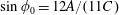$\sin \unicode[STIX]{x1D719}_{0}=12A/(11C)$ . In the pure heaving mode (figure 1 b), the foil oscillates transversely to the free stream such that the $y$ -coordinate of the centreline of the foil $h$ follows the equation

(2.2) $$\begin{eqnarray}h(t)=A\sin 2\unicode[STIX]{x03C0}ft.\end{eqnarray}$$

The oscillating foil in the two-dimensional incompressible Newtonian flow is characterised by three dimensionless parameters, i.e. the width-based Strouhal number

(2.3) $$\begin{eqnarray}\mathit{St}_{D}=\frac{D\,f}{U},\end{eqnarray}$$

the dimensionless amplitude

(2.4) $$\begin{eqnarray}A_{D}=\frac{2A}{D}\end{eqnarray}$$

and the Reynolds number based on the chord length $\mathit{Re}=CU/\unicode[STIX]{x1D708}$ , where $\unicode[STIX]{x1D708}$ is the kinematic viscosity of the fluid. The width-based Strouhal number $\mathit{St}_{D}$ describes the externally imposed frequency and not the natural vortex shedding frequency, and it is sometimes referred to as the Keulegan–Carpenter number. The product of $\mathit{St}_{D}$ and $A_{D}$ is the so-called amplitude-based Strouhal number,

(2.5) $$\begin{eqnarray}\mathit{St}_{A}=\frac{2A\,f}{U}.\end{eqnarray}$$

The amplitude-based Strouhal number can be understood as the ratio between the speed of the foil tip and the speed of the free stream, and it plays a central role in describing the drag–thrust transition (Triantafyllou, Triantafyllou & Gopalkrishnan Reference Triantafyllou, Triantafyllou and Gopalkrishnan1991).

3 Particle vortex method

The numerical simulations were performed using a two-dimensional discrete particle vortex method. The approach is described in detail elsewhere (Walther & Larsen Reference Walther and Larsen1997; Rasmussen et al. Reference Rasmussen, Hejlesen, Larsen and Walther2010), and it has been validated for the flow past a flat plate (Walther & Larsen Reference Walther and Larsen1997; Hejlesen et al. Reference Hejlesen, Koumoutsakos, Leonard and Walther2015) and for the flow past suspension-bridge sections (Larsen & Walther Reference Larsen and Walther1997). The method is based on a Lagrangian formulation of the two-dimensional vorticity equation

(3.1) $$\begin{eqnarray}\frac{\unicode[STIX]{x2202}\unicode[STIX]{x1D714}}{\unicode[STIX]{x2202}t}+(\boldsymbol{v}\boldsymbol{\cdot }\unicode[STIX]{x1D735})\unicode[STIX]{x1D714}=\unicode[STIX]{x1D708}\unicode[STIX]{x1D6FB}^{2}\unicode[STIX]{x1D714},\end{eqnarray}$$

where $\boldsymbol{v}$ denotes the velocity and $\unicode[STIX]{x1D74E}=\unicode[STIX]{x1D735}\times \boldsymbol{v}$ the vorticity. At each time step, the instantaneous fluid velocity is obtained from the Biot–Savart relation

(3.2) $$\begin{eqnarray}\displaystyle \boldsymbol{v}(x,y) & = & \displaystyle \boldsymbol{U}+\frac{1}{2\unicode[STIX]{x03C0}}\iint _{S_{\mathit{fluid}}}\frac{\unicode[STIX]{x1D74E}(x^{\prime },y^{\prime })\times (\boldsymbol{x}-\boldsymbol{x}^{\prime })}{|\boldsymbol{x}-\boldsymbol{x}^{\prime }|^{2}}\,\text{d}x^{\prime }\,\text{d}y^{\prime }\nonumber\\ \displaystyle & & \displaystyle -\,\frac{1}{2\unicode[STIX]{x03C0}}\oint _{C_{\mathit{foil}}}\frac{[\boldsymbol{v}(x^{\prime },y^{\prime })\boldsymbol{\cdot }\boldsymbol{n}(x^{\prime },y^{\prime })](\boldsymbol{x}-\boldsymbol{x}^{\prime })-[\boldsymbol{v}(x^{\prime },y^{\prime })\times \boldsymbol{n}(x^{\prime },y^{\prime })]\times (\boldsymbol{x}-\boldsymbol{x}^{\prime })}{|\boldsymbol{x}-\boldsymbol{x}^{\prime }|^{2}}\,\text{d}l^{\prime },\nonumber\\ \displaystyle & & \displaystyle\end{eqnarray}$$

where $\boldsymbol{n}$ denotes the outward unit normal at the foil boundary, $C_{\mathit{foil}}$ the foil boundary and $S_{\mathit{fluid}}$ the fluid domain. The boundary integral accounts for the vorticity within the foil due to the solid-body rotation. The foil boundary is discretised using boundary elements with vortex sheets of linearly varying strength. In the present study, we discretise the foil boundary using 400 elements and conduct the simulations for 10 periods of the flapping motion. The no-slip boundary condition is imposed by solving a boundary integral equation obtained from (3.2) for the unknown vortex sheet strengths while satisfying Kelvin’s circulation theorem. The vortex sheets are subsequently diffused into the flow to form the no-slip boundary layer. The advection is described by the inviscid motion of the discrete vortex particles, and viscous diffusion is modelled using the method of random walks (Chorin Reference Chorin1973). In the simulations, we have $\mathit{Re}=2640$ to match the experiments (Schnipper et al. Reference Schnipper, Andersen and Bohr2009). To reduce computational costs, the velocity equation (3.2) is computed using the adaptive fast multipole method (Carrier, Greengard & Rokhlin Reference Carrier, Greengard and Rokhlin1988), and vortex particles are amalgamated five chord lengths downstream of the trailing edge. Control simulations without amalgamation show that amalgamation has no effect on the fluid forces acting on the foil.

Figure 2. Wakes of the pitching foil in simulation (colour) and experiment (greyscale). Red (blue) corresponds to positive (negative) vorticity, and the magenta lines show average velocity profiles four chord lengths downstream of the trailing edge, with the black lines showing the inflow velocity as reference. (a) A $2P$ wake ( $\mathit{St}_{D}=0.08$ , $A_{D}=1.14$ and $\langle C_{T}\rangle =-0.12$ ), see also supplementary movie 1 available at https://doi.org/10.1017/jfm.2016.808; (b) a $2P$ wake that evolves to a von Kármán wake ( $\mathit{St}_{D}=0.11$ , $A_{D}=1.14$ and $\langle C_{T}\rangle =-0.12$ ); (c) a von Kármán wake ( $\mathit{St}_{D}=0.12$ , $A_{D}=1.14$ and $\langle C_{T}\rangle =-0.12$ ); (d) an inverted von Kármán wake ( $\mathit{St}_{D}=0.18$ , $A_{D}=1.65$ and $\langle C_{T}\rangle =0.00$ ).

The instantaneous net fluid force on the foil is computed from the equation

(3.3) $$\begin{eqnarray}\boldsymbol{F}(t)=\unicode[STIX]{x1D70C}\frac{\text{d}}{\text{d}t}\left(\iint _{S_{\mathit{foil}}}\boldsymbol{v}\,\text{d}x\,\text{d}y-\iint _{S_{\mathit{fluid}}}\boldsymbol{x}\times \unicode[STIX]{x1D74E}\,\text{d}x\,\text{d}y\right),\end{eqnarray}$$

where $\unicode[STIX]{x1D70C}$ is the density of the fluid and $S_{\mathit{foil}}$ is the domain occupied by the foil (Wu Reference Wu1981; Walther & Larsen Reference Walther and Larsen1997). We shall, for convenience, decompose the net fluid force on the foil into thrust and lift components $F_{T}=-F_{x}$ and $F_{L}=F_{y}$ , and use the standard definitions of the instantaneous thrust and lift coefficients

(3.4a,b ) $$\begin{eqnarray}C_{T}=\frac{F_{T}}{(1/2)\unicode[STIX]{x1D70C}CU^{2}},\quad C_{L}=\frac{F_{L}}{(1/2)\unicode[STIX]{x1D70C}CU^{2}}.\end{eqnarray}$$

From (3.3), we obtain the equation for the thrust component

(3.5) $$\begin{eqnarray}F_{T}=-\unicode[STIX]{x1D70C}\frac{\text{d}}{\text{d}t}\left(\iint _{S_{\mathit{foil}}}v_{x}\,\text{d}x\,\text{d}y-\iint _{S_{\mathit{fluid}}}y\unicode[STIX]{x1D714}\,\text{d}x\,\text{d}y\right).\end{eqnarray}$$

The equation highlights the close connection between the transition from drag to thrust and the transition in the arrangement of the coherent vortices in the wake, e.g. from von Kármán wake with $y$ and $\unicode[STIX]{x1D714}$ predominantly of opposite signs to inverted von Kármán wake with $y$ and $\unicode[STIX]{x1D714}$ predominantly of the same sign (von Kármán & Burgers Reference von Kármán, Burgers and Durand1935).

Figure 3. Wake map for the pitching foil. Experiment (background shades) and simulation (symbols): (○, white) von Kármán wakes, (

, light grey) inverted von Kármán wakes, (▪, black bars) aligned $2S$ wakes with vortices on the symmetry line, (

, dark grey) $2P$ wakes and (♢) periodic vortex wakes with blurry vorticity regions. The yellow discs indicate the cases in figure 2 and the red crosses the examples shown in figure 4. The solid blue curve shows the drag–thrust transition and the dashed black curve shows the contour line with $\mathit{St}_{A}=0.28$ .

4 Pitching foil in experiment and simulation

We first consider the pitching foil in experiment and simulation. We shall label the wakes using the symbols introduced by Williamson & Roshko (Reference Williamson and Roshko1988), where $mS+nP$ signifies $m$ single vortices and $n$ vortex pairs shed per oscillation period. Figure 2 shows a $2P$ wake (a), a $2P$ wake that evolves downstream to a von Kármán wake (b), a von Kármán wake (c) and an inverted von Kármán wake (d). In the simulation images, each dot corresponds to a vortex particle with positive (red) or negative (blue) circulation. Regions with high dot density that are dominated by red (blue) dots correspond to vortices of positive (negative) net circulation. The wake types are identified by visual inspection in the approximate interval 2–4 chord lengths downstream of the trailing edge, and the soap film experiment additionally allows us to use a long 20 chord length interval to follow the downstream wake evolution.

In all four cases, we observe that the vortex particles in the simulation and the thickness variations in the soap film form similar structures, i.e. concentrated vortices connected by narrow curved bands of vorticity. Agreement is also observed in the flow close to the leading and trailing edges, where four patches of vorticity form in every oscillation period. For example, both methods show the formation of two vortex patches, one on each side of the leading edge, per flapping period. After formation, the patches roll downstream along the foil (Schnipper et al. Reference Schnipper, Andersen and Bohr2009). In figure 2(b), we plot an intermediate wake type in which a $2P$ wake evolves downstream to a von Kármán wake by pairwise merging of vortices. We note that a slight decrease of $\mathit{St}_{D}$ yields a stable $2P$ wake, whereas a slight increase yields a von Kármán wake. Differences between simulation and experiment are also observed: the vortices in the inverted von Kármán wake in figure 2(d) are located 18 % closer to each other in the experiment than in the simulation. We presume that this is due to the relatively intense flapping of the foil, which gives rise to compressibility effects in the soap film flow (Chomaz & Cathalau Reference Chomaz and Cathalau1990).

Figure 4. Instantaneous thrust (black) and lift (red) coefficients for the pitching foil in the simulation. (a) von Kármán wake (cf. figure 2 c) with average drag ( $\mathit{St}_{D}=0.12$ and $A_{D}=1.14$ ) and (b) inverted von Kármán wake with average thrust ( $\mathit{St}_{D}=0.22$ and $A_{D}=1.81$ ).

The four wakes in figure 2 are representative of the most significant wake types in the wake map (phase diagram) in figure 3. The symbols indicating periodic wake types in the simulation are plotted on top of the corresponding wake map (shaded areas) measured in the soap film (Schnipper et al. Reference Schnipper, Andersen and Bohr2009). Wakes with no clear periodicity were found in the simulations where symbols are absent in the phase diagram, and in the soap film where the background shade is black. Generally, there is a striking overall agreement in the variety of vortex wakes. Both methods find a region ( $\mathit{St}_{D}>0.1$ ) that is dominated by $2S$ wake types, as observed by Godoy-Diana et al. (Reference Godoy-Diana, Aider and Wesfreid2008), and a region ( $\mathit{St}_{D}<0.1$ ) that is dominated by complex wakes. We observe that the numerical and experimental boundaries between the von Kármán wake and the inverted von Kármán wake correspond well with each other, and only at low frequencies and high amplitudes do we find some quantitative differences. The simulations also reproduce two non-overlapping regions with the $2P$ wake measured in the soap film, i.e. one main region and a small island embedded in the von Kármán region. The $2P$ wakes occur as vortices formed at the leading and trailing edges are shed in turn with a spatial separation sufficiently large to prevent the vortices from merging (Schnipper et al. Reference Schnipper, Andersen and Bohr2009). From animations of the flow fields, it is confirmed that the same process takes place in the simulations. These observations indicate that the boundary layer evolutions in the simulation and in the soap film agree well. The agreement in the horizontal width of the $2P$ island furthermore shows that the spatial threshold for vortex merging is the same in the two methods (Schnipper et al. Reference Schnipper, Andersen and Bohr2009).

Figure 5. Selected wakes of the heaving foil in simulation. Red (blue) corresponds to positive (negative) vorticity, and the magenta lines show average velocity profiles four chord lengths downstream of the trailing edge, with the black lines showing the inflow velocity as reference. (a) A $2P$ wake with average drag ( $\mathit{St}_{D}=0.10$ , $A_{D}=1.40$ and $\langle C_{T}\rangle =-0.03$ ); (b) a $2P$ wake immediately below the drag–thrust transition ( $\mathit{St}_{D}=0.10$ , $A_{D}=1.60$ and $\langle C_{T}\rangle =-0.01$ ); (c) a $2P$ wake with average thrust ( $\mathit{St}_{D}=0.10$ , $A_{D}=1.80$ and $\langle C_{T}\rangle =0.02$ ), see also supplementary movie 2; (d) a $2P+2S$ wake ( $\mathit{St}_{D}=0.06$ , $A_{D}=1.60$ and $\langle C_{T}\rangle =-0.09$ ).

Figure 4 shows the instantaneous thrust and lift for the pitching foil in two representative examples: (a)  $\mathit{St}_{D}=0.12$ and $A_{D}=1.14$ , giving rise to a von Kármán wake and average drag $\langle C_{T}\rangle =-0.12$ , and (b)  $\mathit{St}_{D}=0.22$ and $A_{D}=1.81$ , giving rise to an inverted von Kármán wake and average thrust $\langle C_{T}\rangle =0.18$ . The simulation noise is due to the random walks of the vortex particles (Chorin Reference Chorin1973), and the curves are obtained by applying a 10-point moving average filter to the raw numerical data. The instantaneous lift varies periodically with the period $T$ of the foil motion, and the instantaneous drag varies periodically with half of the period, as expected from the reflection symmetry in the problem. Average thrust is only produced by the pitching foil when it is oscillated with sufficiently high frequency and amplitude to give rise to an inverted von Kármán wake (figure 3). More precisely, the drag–thrust transition (solid blue curve) takes place at $\mathit{St}_{A}=0.28$ (dashed black curve), which is a higher value than the transition between von Kármán wake and inverted von Kármán wake at $\mathit{St}_{A}=0.18$ (Schnipper et al. Reference Schnipper, Andersen and Bohr2009). This observation is in agreement with previous measurements and simulations (Godoy-Diana et al. Reference Godoy-Diana, Aider and Wesfreid2008; Bohl & Koochesfahani Reference Bohl and Koochesfahani2009; Das et al. Reference Das, Shukla and Govardhan2016), whereas inviscid theory predicts a drag–thrust transition as the wake changes from von Kármán wake to inverted von Kármán wake (von Kármán & Burgers Reference von Kármán, Burgers and Durand1935).

5 Heaving foil in simulation

The heaving foil forms a variety of $2P$ wakes (figure 5). For increasing $A_{D}$ , the vortex pairs point still more downstream, indicating an increasing amount of thrust production. Figure 5(a) is, in fact, a case where the foil experiences average drag, figure 5(b) is a case immediately below the drag–thrust transition and figure 5(c) is a case of average thrust production. In addition, figure 5(d) shows a $2P+2S$ wake where six vortices are shed in each flapping period. A similar wake type is found, for quite similar flapping parameters, behind the pitching foil in the soap film (figure 3). However, the two $2P+2S$ wakes differ qualitatively in the sense of rotation of the vortex closest to the centreline. The heaving foil sheds three same-signed vortices per flapping half-period. In contrast, the pitching foil, cf. figure 3(d) in Schnipper et al. (Reference Schnipper, Andersen and Bohr2009), forms wake arrangements with vortices of alternating sense of rotation.

Similarly to the pitching foil, the wake map for the heaving foil consists of a region ( $\mathit{St}_{D}>0.1$ ) dominated by $2S$ wake types and a region ( $\mathit{St}_{D}<0.1$ ) that is dominated by more complex wake types (figure 6). Further, it can be noticed that two non-overlapping regions of $2P$ wake exist in the wake map: a main region that is located at $0.06<\mathit{St}_{D}<0.12$ and a small island at $0.19<\mathit{St}_{D}<0.23$ embedded in the von Kármán wake region. The formation of vortex patches close to the leading and trailing edges appears to be similar to the pitching foil. From animations of the flow field, we measure that a leading-edge vortex rolls downstream along the chord with velocity $0.64U$ . Following the simple model by Schnipper et al. (Reference Schnipper, Andersen and Bohr2009), we obtain the theoretical estimates $\mathit{St}_{D}=0.11$ for the centre of the main $2P$ region and $\mathit{St}_{D}=0.22$ for the centre of the $2P$ island, in reasonably good agreement with the wake map based on the numerical simulations.

Figure 6. Wake map for the heaving foil in simulation: ( $+$ )  $2P+2S$ wakes, (○) von Kármán wakes, (

) inverted von Kármán wakes, (▪) aligned $2S$ wakes, (

) $2P$ wakes and (♢) periodic vortex wakes with blurry vorticity regions. The yellow discs indicate the cases in figure 5 and the red crosses the examples shown in figure 7. The solid blue curve shows the drag–thrust transition and the dashed black curve shows the contour line with $\mathit{St}_{A}=0.16$ .

For the heaving foil, the transition from von Kármán wake to inverted von Kármán wake takes place at lower amplitudes than for the pitching foil (figures 3 and 6). In the upper-right part of the wake map, we find oblique inverted von Kármán wakes (Marais et al. Reference Marais, Thiria, Wesfreid and Godoy-Diana2012; Das et al. Reference Das, Shukla and Govardhan2016). In the region $\mathit{St}_{D}<0.12$ , the wake map has a complex structure. In addition to $2P$ wakes, we observe exotic $2P+2S$ wakes, somewhat scattered in the region. In contrast to the case of the pitching foil, we find a transition from $2P$ wake to inverted von Kármán wake by increasing $\mathit{St}_{D}$ for constant amplitude in the range $1.5<A_{D}\leqslant 2.0$ . We do not observe systematically any von Kármán wake to inverted von Kármán wake transition in this region.

Figure 7. Instantaneous thrust (black) and lift (red) coefficients for the heaving foil in simulation. (a) von Kármán wake with average drag ( $\mathit{St}_{D}=0.11$ and $A_{D}=1.20$ ) and (b) inverted von Kármán wake with average thrust ( $\mathit{St}_{D}=0.22$ and $A_{D}=1.80$ ).

Figure 7 shows the instantaneous thrust and lift for the heaving foil in two representative examples: (a)  $\mathit{St}_{D}=0.11$ and $A_{D}=1.20$ , giving rise to a von Kármán wake and average drag $\langle C_{T}\rangle =-0.03$ , and (b)  $\mathit{St}_{D}=0.22$ and $A_{D}=1.80$ , giving rise to an inverted von Kármán wake and average thrust $\langle C_{T}\rangle =0.39$ . We observe both $2P$ and $2P+2S$ in the thrust region of the heaving foil (figure 6), and we see that an indication of average thrust production is that the vortex pairs in the $2P$ wake point in the downstream direction (figure 5 c). The vortex pairs give rise to average jet flow above and below the symmetry line, in contrast to the inverted von Kármán wake with strong average jet flow on the symmetry line (figure 2 d). Similarly to the pitching foil, we observe that the drag–thrust transition (solid blue curve) closely follows an $\mathit{St}_{A}$ contour line, albeit at the lower value $\mathit{St}_{A}=0.16$ (dashed black line). We note that $2P$ wakes with average thrust, interpreted from slices through three-dimensional vortex rings, have been measured behind freely swimming fish such as bluegill sunfish (Drucker & Lauder Reference Drucker and Lauder2002) and eel (Tytell & Lauder Reference Tytell and Lauder2004). It will be interesting to explore to what extent the results of the present study are applicable to three-dimensional situations.