


1. Introduction
Thermally driven flows play an important role in both nature and industry. They are notoriously hard to predict and control. In the presence of gravity, temperature fluctuations cause density fluctuations, which in turn drive convective motions through buoyancy in the atmosphere (Markowski Reference Markowski2007; Salesky & Anderson Reference Salesky and Anderson2018), in oceans (Marshall & Schott Reference Marshall and Schott1999), and especially in idealized systems such as Rayleigh–Bénard convection (Ahlers, Grossmann & Lohse Reference Ahlers, Grossmann and Lohse2009; Lohse & Xia Reference Lohse and Xia2010) and horizontal convection (Gayen, Griffiths & Hughes Reference Gayen, Griffiths and Hughes2014).
It is well known that the two-way interactions between particles suspended in a fluid and the fluid phase itself are complex and highly nonlinear. They exhibit behaviour such as preferential concentration due to ejection from vortical regions (Squires & Eaton Reference Squires and Eaton1991; Cencini et al. Reference Cencini, Bec, Biferale, Boffetta, Celani, Lanotte, Musacchio and Toschi2006) and modification of turbulence (Yang & Shy Reference Yang and Shy2005). The dynamics of particles suspended in turbulence plays an important role in several natural as well as industrial processes, for example in the dispersal of pollutants (Fernando et al. Reference Fernando, Zajic, Di Sabatino, Dimitrova, Hedquist and Dallman2010), clouds (Mazin Reference Mazin1999; Falkovich, Fouxon & Stepanov Reference Falkovich, Fouxon and Stepanov2002), planet formation (Bec, Homann & Ray Reference Bec, Homann and Ray2014) and combustion of jet sprays (Irannejad, Banaeizadeh & Jaberi Reference Irannejad, Banaeizadeh and Jaberi2015).
When suspended particles are thermally coupled to the fluid and are non-isothermal, the particles cause local temperature fluctuations in the fluid, which in turn can further modify a turbulent flow, either purely by thermal action or also in conjunction with the momentum coupling (Carbone, Bragg & Iovieno Reference Carbone, Bragg and Iovieno2019) while momentum coupling alone can also alter the heat transfer dynamics of a thermal flow (Elperin, Kleeorin & Rogachevskii Reference Elperin, Kleeorin and Rogachevskii1996). Modification of specific thermal flows due to suspended thermal particles has also been studied, for example in Rayleigh–Bénard convection (Park, O'Keefe & Richter Reference Park, O'Keefe and Richter2018), where heavy particles with fixed initial temperatures are introduced into a Rayleigh–Bénard convection system. In this case, the particles are found to enhance vertical heat transfer, an effect that is most pronounced when the particle concentration is greatest due to turbulence (preferential concentration), while attenuating turbulent kinetic energy due to momentum coupling. Furthermore, the feasibility of achieving control of Rayleigh–Bénard convection solely by applying small temperature or velocity fluctuations has been studied (Tang & Bau Reference Tang and Bau1994). Here, deviations from the stable profiles near the thermal boundaries are detected and compensated, leading to stable Rayleigh–Bénard flows well above the critical Rayleigh number, and also the possibility of control of flow patterns is given. Increasing the critical Rayleigh number and delaying the onset of convection can be improved further by applying reinforcement learning techniques to apply the temperature fluctuations near the boundary, as shown by Beintema et al. (Reference Beintema, Corbetta, Biferale and Toschi2020).
External radiation acting solely by heating particles suspended in a flow has been shown to modify the global motion and to induce turbulent thermal convection. The work of Zamansky et al. (Reference Zamansky, Coletti, Massot and Mani2014, Reference Zamansky, Coletti, Massot and Mani2016) considered a transparent fluid with suspended inertial particles subject to a constant radiation and at local thermal equilibrium with the fluid. Convection induced in such a system was found to be driven by individual plumes rising out of each particle, with turbulent kinetic energy being the largest in the presence of a strong particle preferential concentration where the plumes of individual particles are reinforced by one another due to their spatial proximity. This eventually led to a sustained turbulent thermal convection, albeit with the temperature of the system constantly increasing due to the permanently applied incident radiation.
Internally heated convection – induced and sustained by the application of a bulk heating term in a fluid – has also been studied as an idealized theoretical model by Wang, Lohse & Shishkina (Reference Wang, Lohse and Shishkina2021). They consider a uniformly heated domain with the top and bottom walls kept at the same constant temperature. In this scenario, the bulk attains a stationary temperature depending on the strength of the heating and other parameters, such as gravity or the height of the domain, while the fixed temperature boundaries work as sinks of heat, ensuring that the temperature does not increase indefinitely.
The study of fluid systems where the heating in the bulk rather than boundary forcing is the dominant mode of thermal forcing has important implications for several natural systems. For example, in the mantle of the Earth, the radiogenic heating from the decay of radioactive elements plays a significant role in addition to the heat transfer from the hotter inner core (Lay, Hernlund & Buffett Reference Lay, Hernlund and Buffett2008). The atmosphere of Venus, which contains a high amount of sulphurous gases, absorbs a large part of the incoming solar radiation, making this the dominant mode of heat transfer (Tritton Reference Tritton1975), in contrast to the Earth, where the majority of the radiation is absorbed by the land surface and in turn forces the atmosphere. The mantle of Venus is driven in large part by internal heating (Limare et al. Reference Limare, Vilella, Di Giuseppe, Farnetani, Kaminski, Surducan, Surducan, Neamtu, Fourel and Jaupart2015). Finally, in industrial applications, chiefly in the interior of liquid-metal batteries, convection due to internal heating is of crucial importance (Kim et al. Reference Kim2013).
In this study, we set up a ‘theoretical experiment’ to study the possibility of controlling the global properties of a thermal flow by applying temperature fluctuations locally along particle trajectories. In our proposed idealization, the particles are equipped with a hard-wired active protocol capable of releasing or absorbing heat by setting the temperature of each Lagrangian, thermally active tracer as a function of the local velocity field of the underlying fluid background. Our system is internally heated/cooled by these virtual particles, so that the average heating term  $\varPhi$ is statistically zero and hence the average temperature attained by the fluid is unchanged by the forcing. The heat injection by the particles is the only energy source for the system, since the horizontal boundaries are periodic, and the top and bottom walls are adiabatic. The aims of the set-up are many. First, as a proof of concept, we wish to demonstrate that it is possible to invent hard-wired Lagrangian protocols that can cause global flow transitions. Second, we hope to trigger more studies using phenomenological or data-driven approaches to achieve control of complex systems. Finally, by acting on thermal plumes, we hope that one can better understand their role in determining the organization of the global flow.
The remainder of the paper is organized in the following manner. In § 2, we introduce the model equations for the system and the particle temperature protocol, and describe the numerical experiments conducted. In § 3, we present and discuss our main findings from the numerical experiments. Finally, in § 4, we present our conclusions as well as possible future directions for further investigation.
2. Methods
The protocol for particle forcing is as follows. Virtual tracer particles are initially randomly placed in a two-dimensional (2-D) region of length  $L_x$ and height
  $L_z$, with a fluid at rest. The initial temperature of the fluid is set to an unstable configuration, with warmer temperatures at the bottom of the domain, and colder temperatures at the top of the domain. The particles are idealized to have an infinite heat capacity and a temperature determined by an imposed protocol in which rising particles moving vertically upwards are warm with a positive temperature
  $T_+$, while the temperature of falling particles is set to
  $-T_+$ (see figure 1), so the average temperature of the fluid remains constant. The temperature of the fluid near the particle relaxes to the temperature of the particle at a rate proportional to the difference between the local fluid temperature
  $T$ and the particle temperature
  $T_p$, with relaxation time
  $\tau = 1/\alpha$.

Figure 1. An overview of the methods applied in the study. The domain consists of adiabatic walls at the top and bottom, while the lateral boundaries are periodic. Insets (i) and (ii) show a rising hot particle with temperature  $T_+$, and a falling cold particle with temperature
  $-T_+$, respectively.
2.1. Fluid equations of motion
The fluid velocity  $\boldsymbol {u} = (u,v)$ and temperature
  $T$ follow the equations
 $$\begin{gather} \boldsymbol{\nabla} \boldsymbol{\cdot} \boldsymbol{u} = 0, \end{gather}$$
 $$\begin{gather}\partial_t \boldsymbol{u} + (\boldsymbol{u} \boldsymbol{\cdot}\boldsymbol{\nabla}) \boldsymbol{u} ={-} \boldsymbol{\nabla} p + \nu\,\nabla^2 \boldsymbol{u} - \beta T \boldsymbol{g}, \end{gather}$$
 $$\begin{gather}\frac{\partial T}{\partial t} + \boldsymbol{u} \boldsymbol{\cdot} \boldsymbol{\nabla} T = \kappa\,\nabla^2 T - \sum_{i=1}^{N_p} \left(\alpha_i(\boldsymbol{r},t) \left[T(\boldsymbol{r},t) - T_i(t)\right]\right), \end{gather}$$
where (2.1) and (2.2) are the incompressible Navier–Stokes equations for a fluid with unit density and average temperature  $T_0=0$, with a buoyancy force term according to the Boussinesq approximation, where the density variations are small and enter the equations only via the gravity force term. Here,
  $p$ is the fluid pressure,
  $\nu$ is the kinematic viscosity, and
  $\beta$ is the thermal expansion coefficient. Temperature is advected and diffused by (2.3), where
  $\kappa$ is the thermal conductivity, and the last term on the right-hand side is a heat source term (i.e. a thermal forcing) that depends on the particles (see later).
The domain is periodic in the horizontal  $x$-direction, while the top and bottom walls at
  $z=0$ and
  $z=L_z$ are adiabatic with
  $\boldsymbol {u} = 0$, that is,
 $$\begin{gather} \partial_z T |_{z=0} = \partial_z T |_{z=L_z} = 0, \end{gather}$$
 $$\begin{gather}\boldsymbol{u}(z=0) = \boldsymbol{u}(z=L_z) = 0. \end{gather}$$
Note that the only source of energy injected into the system is the heat supplied by the particles.
2.2. Equations of particle motion
Each particle is assumed to be a point-like, thermally active tracer. The  $N_p$ particles with positions
  $\{\boldsymbol {r}_1,\boldsymbol {r}_2,\dots,\boldsymbol {r}_{N_p}\}$ and temperatures
  $\{ T_1, T_2, \ldots, T_{N_p}\}$ follow the local fluid velocity
 \begin{equation} \frac{{\rm d}\boldsymbol{r}_i}{{\rm d}t} = \boldsymbol{u}(\boldsymbol{r}_i(t),t). \end{equation}
 To mimic an effective particle size, concerning its thermal properties, we imagine that each particle exerts a thermal forcing on the fluid in its immediate vicinity up to a cut-off distance  $\eta$. The feedback of the particle is defined as a local heat injection term proportional to the difference between the underlying fluid temperature, at the location of the particle, and the instantaneous particle temperature. Furthermore, to have a smooth thermal forcing, we assume that the strength of the coupling
  $\alpha _i$ (with dimension inverse of time) between the
  $i$th particle and the fluid at time
  $t$ and position
  $\boldsymbol {r}$ has the form of a Gaussian with a peak at the particle location
  $\boldsymbol {r}_i(t)$, given by
 \begin{equation} \alpha_i(\boldsymbol{r},t)= \begin{cases} \alpha_0 \exp{\left(-\dfrac{|\boldsymbol{r} - \boldsymbol{r}_i(t)|^2}{2c^2} \right)}, & \text{if } |\boldsymbol{r} - \boldsymbol{r}_i(t)| \le\eta,\\ 0, & \text{if } |\boldsymbol{r} - \boldsymbol{r}_i(t)| > \eta. \end{cases} \end{equation}
Here,  $\alpha _0$ is the coupling strength at the particle location, and
  $c$ is the size of the virtual particle (referred to as particle size). In fact,
  $c$ determines the sharpness of the peak of the Gaussian function
  $\alpha _i$: the Gaussian peaks more sharply and falls off more quickly for smaller
  $c$. On the other hand,
  $\eta$ is simply a cut-off length for the thermal forcing by the particle. While setting a cut-off length introduces a discontinuity in the system, we note that for the typical parameters chosen in the study, the value of
  $\alpha$ at the cut-off length is
  $\approx 0.011 \alpha _0$. This value is only
  $1$% of the value at
  $\boldsymbol{r} = \boldsymbol{r} _i$. The cut-off is used to save computational resources and to avoid calculating vanishingly small values of the Gaussian curve for points far away from a particle (large values of
  $|\boldsymbol {r} - \boldsymbol {r}_i|)$.
The thermal forcing due to the  $i$th particle
  $\varPhi _i$ at location
  $\boldsymbol {r}$ is
 \begin{equation} \varPhi_i(\boldsymbol{r},t) ={-} \alpha_i (\boldsymbol{r},t) \left[T(\boldsymbol{r},t) - T_i (t) \right], \end{equation}
and the total thermal forcing at a given location  $\boldsymbol {r}$ due to all
  $N_p$ particles reads
 \begin{equation} \varPhi(\boldsymbol{r},t) ={-} \sum_{i=1}^{N_p} \left(\alpha_i(\boldsymbol{r},t) \left[T(\boldsymbol{r},t) - T_i(t)\right]\right). \end{equation}
Here,  $\varPhi (\boldsymbol {r},t)$ is of exactly the same form as (2.3). It defines the relationship between the particle positions and the thermal forcing at a given location in the fluid, and thus can be directly substituted into the heat equation, which is an Eulerian description of the temperature.
To summarize, each particle influences a fixed region surrounding itself, and when two particles are within distance  $2\eta$, their thermal effects are additive in the overlapping region. The coupling between the particle and the fluid is two-way, since the particle actively heats or cools the fluid, while the fluid acceleration due to this thermal forcing also accelerates the particle.
2.3. Particle temperature policy
The temperatures of the particles are determined by a binary policy where the  $i$th particle has either a positive value
  $T_+$ or a negative value
  $-T_+$ depending on the sign of the vertical velocity of the particle
  $v_i(t)$:
 \begin{equation} T_i = \begin{cases} T_+ , & \text{if } v_i > 0,\\ -T_+ , & \text{if } v_i < 0. \end{cases} \end{equation}
Since the particle is a tracer,  $v_i$ is the same as the vertical velocity of the fluid at the particle location
  $v(\boldsymbol {r}_i,t)$. Here,
  $T_+$ is a parameter that sets the temperature scale of the system. By heating the upward moving fluid regions, and conversely cooling the downward moving regions, this policy should enhance thermal convection by amplifying any updrafts or downdrafts if they exist. Particles are coupled to each other via their effects on the fluid and because of the flow thermal diffusivity.
Our policy leads to a sharp discontinuity in the particle temperature when the particle changes direction. Furthermore, the temperature would fluctuate rapidly between  $T_+$ and
  $-T_+$ at the top and bottom walls, where the velocity is very small and the flow is mainly horizontal. To ensure that this does not affect our results, we verified that setting
  $T_i = 0$ for particles within one grid length from the top and bottom walls, where the vertical velocity of the particle fluctuates rapidly from small positive values to small negative values, leads to (statistically) the same flows. We have also verified that all results reported below are robust against small changes of the above protocol, e.g. by setting a threshold velocity
  $v_0$ such that
  $T_i=0$ when
  $|v|< v_0$.
2.4. Numerical experiments
The fluid equations (2.1)–(2.3) are solved by the lattice Boltzmann method (see Appendix A for details), together with the particle evolution as a tracer given by (2.6). The particle evolution is solved by the two-step Adams–Bashforth method. We start from an initially unstable vertical temperature profile
 \begin{equation} T(z) = T_+ \tanh \left( \frac{L_z}{2} - z \right) . \end{equation}
The two-way coupled particle–fluid system is evolved until the flow reaches a statistically stationary kinetic energy independent of the initial conditions for the flow velocity, temperature and particle positions. All measurements and analyses are performed at this steady state for different sets of parameters, varying  $T_+$,
  $N_p$,
  $\alpha _0$ and
  $c$. The cut-off distance for the particles
  $\eta$ is kept constant throughout the study.
All results presented in this study are for a 2-D fluid domain resolved with 864 grid points in the horizontal direction and 432 grid points in the vertical direction. With the lattice Boltzmann grid spacing  $\Delta x = 1$, we have
  $L_x = 864$ and
  $L_z = 432$. The particles have a fixed cut-off distance
  $\eta = 3$ in computational units, while their size
  $c$ is varied. Here,
  $\alpha _0$ is varied from
  $10^{-4}$ to
  $5 \times 10^{-3}$ in simulation units. The temperature
  $T_+$ is varied over several orders of magnitude. All temperatures in this study are reported in units of
  $T_s/0.025$, where
  $T_s$ is the temperature in simulation units. Thus
  $T = 0.1$ corresponds to a temperature
  $T_s = 0.0025$ in simulation units. This convention is chosen solely to make it easier to compare the scales of the various
  $T_+$ and make the paper more readable. The values of the parameters are summarized in table 1.
Table 1. List of parameters used in the study, along with the ranges of values in simulation units.

In order to have dimensionless quantities, we define a typical velocity  $u_0$ given by
 \begin{equation} u_0 = \sqrt{c g \beta\,\frac{\alpha_0}{\alpha_0 + \dfrac{\kappa}{2c^2}}\,T_+}, \end{equation}
where  $c$ is the size of the particle as defined in (2.7). The form (2.12) was suggested by studying the evolution of single-particle experiments at varying
  $\alpha _0$ and
  $c$, where the r.m.s. value of the vertical particle velocity was found to scale as in (2.12). In particular, we find that the particle velocity statistics remain independent of the domain height
  $L_z$, justifying the choice of
  $c$ as the length scale of the system. The fluid near the particle relaxes to the temperature of the particle, and this relatively hotter/cooler local plume rises/falls. The tracer particle in turn responds to the fluid and accelerates at a rate that depends on the temperature anomaly, gravity
  $g$ and
  $\beta$. This is similar to other thermal flows, such as Rayleigh–Bénard convection. The local heating is high when
  $c$ is large because a wider region around each particle is forced thermally.
In the given protocol, the temperature scale alone is set by the particles, and this in turn sets a natural velocity field for the system. Given that the particles are active and the fluid–particle coupling is highly nonlinear, it would be a hard task to estimate other quantities associated with thermal systems usually defined in the literature, such as a Richardson number or a Brunt–Vaisala frequency, as this would require a priori knowledge of the average state of the system.
The quantity
 \begin{equation} T_a = \frac{\alpha_0}{\alpha_0 + \dfrac{\kappa}{2c^2}}\,T_+ \end{equation}
is interpreted as an effective temperature reached in the vicinity of each particle. The empirical prefactor  $\alpha _0/(\alpha _0 + (\kappa /2c^2))$ by which
  $T_+$ is multiplied is a constant that gives the rate of relaxation of the fluid temperature to the particle temperature compared with the rate at which heat is diffused away from the particle by conduction, which is proportional to
  $\kappa /c^2$. When
  $\alpha _0\to 0$, we have
  $T_a\to 0$, because the fluid is no longer coupled to the particle and there is no energy input to the system. When
  $\alpha _0 \gg \kappa /c^2$, we have
  $T_a\to T_+$, meaning that the fluid attains the local particle temperature. For large
  $\kappa$, the heat is conducted rapidly away from the particle so that the effective temperature is lower, where again
  $T_a\to 0$ when
  $\kappa \to \infty$, while the case of small
  $\kappa$ is similar to that of large
  $\alpha _0$. In our study,
  $\alpha _0$ and
  $\kappa /c^2$ are of comparable magnitude.
Furthermore, we define the normalized turbulent kinetic energy  $E_k(t)$ of the system as
 \begin{equation} E_k(t) = \frac{1}{2}\,\frac{\left\langle |\boldsymbol{u}(t)|^2 \right\rangle_V}{u_0^2 N_p}, \end{equation}
where  $\langle \cdot \rangle _V$ represents the average over the entire domain at a given time. We also define (with an overline)
  $\bar {E}_k$ as the average normalized turbulent kinetic energy (TKE), i.e.
 \begin{equation} \bar{E}_k = \left\langle E_k(t) \right\rangle_t, \end{equation}
where  $\langle \cdot \rangle _t$ denotes the time average after the flow reaches a statistically stationary regime. If the particles are sparse and their motion is independent of each other, then the kinetic energy of the system would simply be a sum of the motion of the individual particles and we would expect
  $\bar {E}_k$ of the flow to attain a constant value. However, if the motions of the particle are not independent of each other, then the variation of
  $\bar {E}_k$ as a function of
  $N_p$ is not possible to predict a priori.
3. Results
3.1. Stable and convective configurations
First, we vary the number of virtual particles  $N_p$. Figure 2 shows four cases, where we visualize snapshots of the temperature and velocity fields. Thereby the rising particle temperature
  $T_+$, particle–fluid coupling strength
  $\alpha _0$, and particle size
  $c$ are fixed. The figure indicates that there are two distinct stationary typical configurations. The first, which we term stable, is shown in figures 2(a,b). In this state, kinetic energy is low and large-scale circulation is absent. Particles either are nearly still and close to the top and bottom walls, or execute a slow vertical motion independently one from the others, propelled by their higher or lower temperature compared to the bulk. When the particle concentration reaches beyond a certain threshold, the individual thermal effect of the particles aggregates and triggers a transition to a second state, shown in figures 2(c,d). This convective state enjoys a large-scale circulation and the presence of rising and falling plumes, with the particle trajectories synchronized with the large-scale recirculation regions. In figure 2, this transition occurs for
  $N_p \sim 150$.

Figure 2. Snapshots of the temperature field  $T(\boldsymbol {r},t)/T_+$ at a given instant of time for
  $T_+ = 0.1$,
  $\alpha _0 = 0.005$,
  $c=1$, and at changing
  $N_p = 120,140, 160,180$ in (a–d), respectively. The colour palette varies from red to blue, where red indicates
  $T = T_+$, and blue indicates
  $T = -T_+$. The black arrows show the velocity field, with the length of the arrow representing the relative magnitude of the velocity, with identical scaling for (a–d). Panels (a,b) show a stable configuration, while (c,d) show a convective configuration.
In figure 3, we show the time evolution of the TKE for parameters before and after the transitions. Figures 3(a), 3(b) and 3(c) correspond to  $T_+ = 0.02$,
  $T_+ = 0.1$ and
  $T_+ = 1.0$, respectively, with
  $\alpha _0$ and
  $c$ remaining fixed. The blue curves represent stable configurations while the red curves represent convective configurations. The kinetic energy first increases due to the unstable temperature gradient imposed on the initial condition. At later times, the thermal forcing by the tracers is dominant and the flow attains a statistically stationary kinetic energy where
  $E_k(t)$ either shows a large value (red curves), corresponding to a convective flow shown qualitatively in figure 2 or a low value (blue curves) corresponding to a quasi-stable flow.

Figure 3. Time evolution of  $E_k(t)$ for flows with (a)
  $T_+ =0.02$, (b)
  $T_+0.1$, and (c)
  $T_+=1.0$, with
  $\alpha _0 = 0.005$ and
  $c = 1$ kept fixed. Stable configurations are plotted in blue, while convective configurations are plotted in red. The time is in simulation time units.
Two further points are noteworthy about the transition from figure 3. First, the transition is abrupt: it is enough to add very few particles to have a jump  $\gtrsim 5$ in the normalized kinetic energy. It should be noted that the expression of
  $E_k(t)$ is normalized by
  $N_p$ in the denominator, so the absolute increase in kinetic energy is even greater. Second, the critical
  $N_p$ depends slightly on
  $T_+$, where for larger
  $T_+$, the transition occurs at a slightly larger
  $N_p$. We see that in figure 3(a) with
  $T_+ = 0.02$, the transition lies between
  $N_p = 120$ and
  ${N_p = 140}$, while in figure 3(c) with
  $T_+ = 1.0$, the transition lies between
  $N_p = 160$ and
  ${N_p = 180}$, with the case of
  $T_+ = 0.1$ in figure 3(b) showing an intermediate behaviour. This weak dependence on
  $T_+$ will be commented upon further later. It has been verified that the transitions are robust by replacing the initial unstable profile with an initial temperature field of
  $T=0$ everywhere with particles being either hot or cold with probability
  $0.5$ each.
In figure 4, we show a comparison of the normalized time-averaged vertical temperature profiles  $\bar {T}(z)$ for the same set of flows given by
 \begin{equation} \bar{T}(z) = \frac{\left\langle T(\boldsymbol{r},t) \right\rangle_{x,t}}{T_+}, \end{equation}
where  $\langle \cdot \rangle _{x,t}$ represents the time average at a given height
  $z$. Notice that the temperature gradients for the stable flows (blue) show a strongly stable profile (
 $\partial _z T > 0$), while the convective flows still show an overall stable temperature profile but with weaker gradients so that the temperature difference between the top and the bottom adiabatic walls is much smaller. In the presence of a large-scale circulation, the temperature field is more effectively transported and mixed throughout the domain. We also see that with increase in
  $T_+$, the convective configurations show a flatter temperature profile for the corresponding
  $N_p$ of lower
  $T_+$ flows, i.e. for example, the red curves in figure 4(c) are much flatter than those in figure 4(a).

Figure 4. Time-averaged vertical temperature profile divided by  $T_+$ plotted against the vertical height for various
  $N_p$ close to the transition
  $N_p$ for (a)
  $T_+ = 0.02$, (b)
  $T_+ = 0.1$, and (c)
  $T_+ = 1.0$. Stable configurations are plotted in blue, while convective configurations are shown in red.
The dual nature of the effect of the virtual particles is observed here – the particles tend to make the flow more stable by carrying heat away from the lower half of the domain, while carrying heat towards the upper half of the domain. Thus the larger  $T_+$ is, the more stable the system becomes. However, when a certain threshold of particles is reached, the situation changes – the virtual particles together create a persistent large-scale flow, and now the convection is strong enough to overcome the stable temperature gradient.
In figure 5, we take a closer look at the transition by plotting the average normalized TKE of the flows as defined in (2.15) against  $N_p$, for the same
  $\alpha _0$ as above, for various
  $T_+$. Here, we see that
  $\bar {E}_k$ initially remains constant for small values of
  $N_p$ and then increases rapidly during the transition from a stable flow to a convective flow. Once the convective flow has been set up, the value of
  $\bar {E}_k$ saturates to a higher constant value for large
  $N_p$. The sharp increase of TKE at a transition
  $N_p$ is once again clearly visible. We empirically define a value
  $E^0_k = 0.225$ indicated by the horizontal red line as the transition point where for stable end states,
  $\bar {E}_k < E^0_k$, and vice versa for the convective end state. The sharpness of the transition is examined more closely in the inset of the figure for a given
  $T_+$. It is seen that the transition occurs for an increase of just a single particle. The dependence of the transition on
  $T_+$ is weak; for
  $T_+$ varying over 2 orders of magnitude, the transition occurs at nearly the same
  $N_p$.

Figure 5. Time-averaged normalized TKE  $\bar {E}_k$ as a function of
  $N_p$ for various
  $T_+$ (shown in legend) for
  $\alpha _0 = 0.005$ and
  $c = 1$. The inset (in the lower right corner) shows the behaviour of a flow with
  $T_+ = 0.1$ very close to the transition
  $N_p$. Also shown are instantaneous snapshots of the temperature field for a stable configuration (bottom) and a convective configuration (top right). The error bars indicate the standard deviation of the temporal fluctuations of
  $E_k(t)$ around the average kinetic energy in the stationary regime.
3.2. Large-scale circulation and heat transfer
While the existence of the large-scale circulation is apparent from the visualizations of the temperature and velocity fields, it is possible to infer its presence quantitatively from the fluid energy spectrum. In particular, we consider the spectrum in the horizontal direction taken at the mid-plane  $z_0 = L_z/2$, given by
 \begin{equation} E_{\boldsymbol{u}}(k_x) = \frac{1}{2} \left\langle \left|\hat{\boldsymbol{u}}(k_x,z_0,t)\right|^2 \right\rangle_t, \end{equation}
where  $\hat {\boldsymbol {u}} (k_x,z_0,t)$ are the Fourier coefficients of the field
  $\boldsymbol {u}$, and
  $\langle \cdot \rangle _t$ denotes time averaging. We denote by
  $E_1$ the energy contained in the first Fourier mode with wavenumber
  $k_x = 2{\rm \pi} /L_x$;
  $E_2$ is used for the energy of the second mode (
 $k_x = 4 {\rm \pi}/L_x$); and so on. Moreover, we define
  $E_{tot}$ as the sum of the energy contained in all the Fourier modes:
 \begin{equation} E_{tot} = \sum_{i=1}^{N_k} E_i, \end{equation}
where  $N_k$ is the Fourier mode corresponding to the smallest resolved length scale. The strength of the large-scale circulation with a rising plume and a falling plume can be measured by the value
  $E_1/E_{tot}$ (Xi et al. Reference Xi, Zhang, Hao and Xia2016), which measures the fraction of energy contained in the first mode, that is, the smallest wavenumber. This corresponds to a cosine mode for the velocity field in the bulk, which is a close approximation when there exist two counter-rotating vortices. When such a large-scale flow is present, we would have
  $E_1/E_{tot} \gg 0$, while if the flow lacks large-scale convection, then we would have a flatter energy spectrum with
  $E_{tot} \gg E_1$ and
  $E_1\sim E_2$.
In figure 6(a), we plot the strength of the large-scale circulation  $E_1/E_{tot}$ for varying
  $N_p$. We see clearly here that corresponding to a jump in the magnitude of the TKE seen in figure 5, there is also a similar large increase in the ratio of kinetic energy contained in the largest scale. Given that
  $\bar {E}_k$ takes into account the typical velocity of a single particle as well as the number of particles, the excess kinetic energy clearly comes from the large-scale circulation that arises after the transition, a cumulative particle effect.

Figure 6. (a) Plots of  $E_1/E_{tot}$ for varying
  $N_p$ for various values of
  $T_+$. Error bars show the temporal fluctuations of
  $E_1/E_{tot}$. (b) Plots of
  ${Nu}$ for varying
  $N_p$ for various values of
  $T_+$. The black solid line shows a linear scaling with
  $N_p$. (c) Plot of the average normalized Nusselt number
  ${Nu}_\varPhi$ against the average normalized thermal energy injection
  $\bar {\epsilon }_T$ for flows with varying parameters. Stable flows are marked with blue filled circles, convective with red filled hexagons, and the two black lines scale as
  $(\bar {\epsilon }_T)^{1.2}$. Inset of (c) shows the scaling of
  ${Nu}_\varPhi$ as a function of
  $N_p$ for three different
  $T_+$.
Figure 6(b) shows the dimensionless Nusselt number  ${Nu}$, defined as
 \begin{equation} {Nu} = \frac{\left\langle v T - \kappa\,\dfrac{\partial T}{\partial z} \right\rangle_{V,t}}{\dfrac{\kappa\,\overline{\Delta T}}{L_z}}, \end{equation}
where  $\langle \cdot \rangle _{V,t}$ represents average over the entire domain and time,
  $v$ is the vertical fluid velocity, and
  $\overline {\Delta T}$ is the time-averaged temperature difference between the top and bottom walls given by
 \begin{equation} \overline{\Delta T} = \left \langle T(x,L_z) \right \rangle_{x,t} - \left \langle T(x,0) \right \rangle_{x,t}. \end{equation}
Here, the Nusselt number is defined in analogy with Rayleigh–Bénard convection: it is the ratio of heat transfer due to convection and the heat transfer by conduction, with the difference that the temperature jump is taken in the opposite sense because of the presence of a stable mean profile. Due to the adiabatic boundary conditions imposed at the top and bottom walls ( $\partial _z T = 0$) along with the no-slip boundary condition for the velocity (
 $\boldsymbol {u} = 0$), the value of the Nusselt number is
  $0$ at the top and bottom walls. Thus the boundary walls do not contribute to the heat transfer. The Nusselt number naturally increases proportionally with the number of particles.
We see in figure 6(b) that the value of  ${Nu}$ increases gradually with increase in
  $N_p$, followed by a large increase around the transition
  $N_p$, and then settling to a roughly linear increase with
  $N_p$ in the convective regime. The reason for the large increase of
  ${Nu}$ at the transition is twofold. First, the increase in TKE overall leads to an increase in the convective heat transfer, which further increases
  $vT$. Second, with more effective mixing of the temperature and a weakly stable temperature gradient,
  $\overline {\Delta T}$ in the denominator also has a smaller magnitude.
Another way to quantify the heat transfer is to divide it by the typical forcing  $\varPhi$ multiplied by the length scale of the system. This is similar to the normalization procedure of (Wang et al. Reference Wang, Lohse and Shishkina2021) applied to internally heated convection (with volume forcing). The effective temperature
  $T_a$ defined in (2.13) was introduced as a typical value of the temperature attained by the fluid in the vicinity of the particle with an associated length scale
  $c$ for each particle. In a similar vein,
  $\alpha _0 (T_+ - T_a)$ can be considered the typical thermal forcing acting on the fluid. We use two dimensionless response parameters of the system. First, we define the normalized Nusselt number
  ${Nu}_{\varPhi }$ given by
 \begin{equation} {Nu}_{\varPhi} = \frac{\left\langle v T - \kappa\,\dfrac{\partial T}{\partial z} \right\rangle_{V,t}}{c \alpha_0 (T_+{-} T_a)}, \end{equation}
where  ${Nu}_{\varPhi }$ measures the heat transfer by convection relative to the input typical thermal forcing multiplied by the length scale of the system.
In the stationary regime, the thermal dissipation rate  $\epsilon _T$ is given by
  $\langle \varPhi T \rangle _{V,t}$ (see Appendix C) and is normalized as
 \begin{equation} \bar{\epsilon}_T = \frac{\langle \varPhi T \rangle_{V,t}}{\alpha_0 (T_+ - T_a) T_+}. \end{equation}
The normalization factor is once again the typical forcing multiplied by the temperature scale.
In figure 6(c), we plot the normalized Nusselt number  ${Nu}_{\varPhi }$ against the normalized thermal dissipation
  $\bar {\epsilon }_T$, quantifying the measured convective response of the fluid to the measured input thermal forcing for varying
  $T_+$,
  $c$,
$c$,  $\alpha _0$ and
  $N_p$. It is seen that there exists a global scaling of these two quantities for both the flow regimes, stable and convective, with a rough scaling
  ${Nu}_{\varPhi } \propto (\bar {\epsilon }_T)^{1.2}$. However, the higher magnitude of the normalized Nusselt number in the convective case differentiates it from the stable flows. In the inset of figure 6(c), we can see that
  $Nu_{\varPhi }$ also shows a transition and a sharp increase in magnitude from stable to convective.
The above findings are consistent with a situation that can be described briefly as: individual particles thermally coupled to the fluid have a small zone of influence and release or absorb heat in their immediate vicinity. Thus each particle contributes to the thermal injection into the domain as well as the vertical heat transfer across the domain, both of which increase with the increase in number of particles. In the stable regime, the main effect of the particles is to maintain the strongly stable temperature gradient. However, since there exists maximum and minimum temperatures that the fluid can attain ( $T_+$ and
  $-T_+$, respectively), there is consequently a limit on the strength of the positive temperature gradient that can be set up in the system, independent of the number of particles. Hence increasing the number of particles eventually leads to a saturation of the stable temperature gradient, while it continues to further destabilize the system. Thus eventually, at a critical
  $N_p$, the instability dominates the flow and leads to a transition to a fully convective flow.
At the transition to the convective regime, the development of the large-scale convective flow patterns and more turbulent flow leads to a large increase in the heat transfer relative even to the thermal energy injection, while also seeing a weaker stable vertical temperature gradient across the domain.
3.3. Particle kinetic energy
Given that the particles are not passive and are actively interacting with the fluid, their behaviour is of particular interest. We define the Lagrangian kinetic  $\bar {E}_{k}^{(L)}$ as
 \begin{equation} \bar{E}_{k}^{(L)} = \frac{1}{u_0^2 N_p} \left \langle \sum_{i=1}^{N_p} \frac{1}{2} \left( u_i^2 + v_i^2\right) \right\rangle_t, \end{equation}
where  $u_i$ and
  $v_i$ are the horizontal and vertical velocities of the
  $i$th particle, respectively. Here,
  $\bar {E}_{k}^{(L)}$ measures the average kinetic energy of a particle in the system. In figure 7, we plot this value against
  $N_p$ for various
  $T_+$, which shows the characteristic jump at the transition to a convective flow. The absolute value of
  $\bar {E}_{k}^{(L)}$ is far larger than the corresponding fluid kinetic energy
  $\bar {E}_k$ due to the fact that the particle locations are the active regions of the flow where the energy is input into the system. Thus, in spite of being tracers, these particles selectively sample higher kinetic energy regions of the flow. Also,
  $\bar {E}_{k}^{(L)}$ shows an increase as a function of
  $N_p$. The reason for this behaviour is twofold. First, with increasing
  $N_p$, the fluid becomes more energetic and turbulent, as discussed before. Second, the particles themselves are better mixed and are found more often in the more energetic regions of the fluid, away from the stationary walls.

Figure 7. Average particle kinetic energy  $\bar {E}_{k}^{(L)}$ plotted against
  $N_p$ for three values of
  $T_+$. All measurements are made with
  $c=1$ and
  $\alpha _0 = 0.005$.
3.4. Comparison with Eulerian imposed thermal forcing
We consider a thermal fluid system with a thermal forcing  $\varPhi (z)$ applied uniformly at all times. The forcing is a close approximation of the vertical profile of the measured forcing
  $\varPhi$ in the Lagrangian system, as shown in figure 8. Defining
  $Q(z)$, the numerator of the Nusselt number, as the average net heat transfer in the positive
  $z$-direction at height
  $z$ given by
 \begin{equation} Q(z) = \left\langle v(\boldsymbol{r},t)\,T(\boldsymbol{r},t) - \kappa\,\partial_z T |_{(\boldsymbol{r},t)} \right\rangle_{x,t}, \end{equation}
where  $\langle \cdot \rangle _{x,t}$ indicates the time and spatial averages at a given height
  $z$, notice that averaging (2.3) over time gives
 \begin{equation} \varPhi(z) := \left\langle\varPhi(\boldsymbol{r},t) \right\rangle_{x,t} = \partial_z Q (z). \end{equation}
Figure 8. The measured value of the average vertical profile of thermal forcing  $\varPhi (z)$ for (a) a stable Lagrangian flow, and (b) a convective Lagrangian flow, shown along with the profile of the corresponding applied Eulerian thermal forcing.
The comparison is made for one stable and one convective flow. Given identical vertical profiles of thermal forcing (see figure 8), one would expect that the resulting temperature profile and hence the nature of the flows would remain identical. However, as shown in figure 9, the temperature profiles show a dramatic difference, with the Eulerian flows showing an unstable temperature profile similar to Rayleigh–Bénard convection. Further, as shown in figure 10, even when the thermal forcing matches the measured value from a stable configuration, the Eulerian flow with uniform thermal forcing shows a convective behaviour with clear, well-defined hot and cold plumes, and an unstable temperature gradient. Even in the convective Lagrangian case, the corresponding Eulerian flow is convective. Thus the presence of the stable temperature gradients and the two typical configurations outlined previously is a result not of the net thermal forcing applied on the system but of the particular Lagrangian nature of the thermal tracers and the two-way coupling with the fluid.

Figure 9. (a) The normalized temperature profile for a stable Lagrangian flow (blue) compared with the measured temperature profile of a flow with an identical imposed profile of thermal forcing. (b) The normalized temperature profile for a convective Lagrangian flow (red) compared with the measured temperature profile of a flow with an identical imposed profile of thermal forcing.

Figure 10. Snapshots of the temperature fields: (a) a stable Lagrangian flow, (c) a convective Lagrangian flow, and the two uniformly forced flows to mimic the (b) stable and (d) convective flows. The temperature fields  $T$ are divided by the respective
  $T_+$. The black arrows show the velocity field. The lengths of the arrows indicate the magnitude of the velocity field – the arrow lengths are scaled differently for different flows to allow for the clearest viewing of the flow structure.
While it is possible to obtain a stable flow by imposing a comparatively very small value of thermal forcing in the Eulerian case, it should be emphasized here that the Lagrangian forcing is a measured quantity and not a quantity that can similarly be set independently. The thermal forcing in the Lagrangian case is not known a priori due to the nonlinear, two-way coupling between the particles and the fluid.
3.5. Anomalous behaviour for small  $T_+$
$T_+$

We have already noted in previous sections that there is weak dependence of the transition of the system on the value of  $T_+$. In particular, it was observed that for larger
  $T_+$, the transition occurs at a larger
  $N_p$, and the stable configurations for larger
  $T_+$ have relatively flatter temperature gradients. One would conclude, then, that for any given
  $N_p$, there exists a
  $T_+$ small enough such that the system is convective. However, at very small
  $T_+$, the system attains a third columnar state where the temperature profile is still stable (
 $\partial _z T>0$) and the system has a weak convective flow (see the snapshot in figure 11b).

Figure 11. (a) The ratio of kinetic energy contained in the first Fourier mode  $E_1/E_{tot}$ (dashed lines) and
  $E_2/E_{tot}$ (solid lines) to the total energy contained in all modes for
  $N_p = 140$ and
  $240$ plotted against
  $T_+$. Inset shows the averaged normalized TKE
  $\bar {E}_k$ for the same parameters, and the horizontal line represents
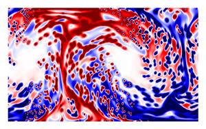
  $\bar {E}_k = E_k^0$. (b) A snapshot of the temperature field for a columnar flow with
  $N_p = 240$ and
  $T_+ = 10^{-5}$. The colour palette varies from red to blue, where red indicates
  $T = T_+$, and blue indicates
  $T = -T_+$.
In figure 11(a), we plot the fraction of energy contained in the first Fourier mode ( $E_1/E_{tot}$) as well as the second Fourier mode (
 $E_2/E_{tot}$) to understand the large-scale behaviour of the flow. We can see clearly that for smaller
  $T_+$, the second mode dominates the kinetic energy, while the energy contained in the first mode approaches
  $0$. This is the case until a transition
  $T_+$, where now the flow turns convective from columnar, with a dominance of
  $E_1$. At larger
  $T_+$ for
  $N_p = 240$ (orange, filled symbols), we see that while
  $E_2/E_{tot}$ remains small, the value of
  $E_1/E_{tot}$ shows a decreasing trend. This is because as
  $T_+$ is increased, the flow becomes more turbulent and small-scale velocity features begin to appear, increasing the energy contained at higher modes. For
  ${N_p = 140}$ (cyan, empty symbols), the flow is columnar for
  $T_+ \lesssim 10^{-3}$ and transitions to convective at
  $T_+ \sim 0.02$, as evidenced by the values of
  $E_1/E_{tot}$ and
  $E_2/E_{tot}$. However, on increasing
  $T_+$ further, the flow again moves to a stable configuration, as evidenced by the fact that
  $E_1 \sim E_2$, which indicates the lack of any large-scale velocity flow. This transition is due to the effect already observed, that for increasing
  $T_+$, the
  $N_p$ of transition from stable to convective is greater.
The inset of figure 11(a) shows the normalized TKE plotted for the two given  $N_p$ and varying
  $T_+$. Notice that at small
  $T_+$, when the flow is columnar, it is characterized by a smaller normalized TKE, and kinetic energy approaches
  $0$ smoothly as
  $T_+ \to 0$.
4. Conclusions and discussion
We have performed numerical simulations of an idealized non-isothermal 2-D fluid system under the Boussinesq approximation with suspended tracer particles. The particles act as heat sources or sinks depending on their vertical velocity. The particles are coupled to the fluid only thermally, and the fluid is forced only by the action of the particles. Individually, each particle aids in the transport of heat away from the bottom of the domain towards the top of the domain, thus working to create a thermally more stable system. However, under certain conditions, the cumulative effect of the particles overpowers the tendency towards stability, and the result is a system with a large-scale convective flow pattern with increased turbulent kinetic energy, larger heat transfer across the domain, maximum energy in the largest Fourier modes, and a (weakly) stable vertical temperature gradient. The main parameters of the system are the temperature of the hot, rising particles  $T_+$, the number of particles
  $N_p$, the strength of the thermal coupling between the fluid phase and the particles
  $\alpha _0$, and the size of the particle
  $c$. Increasing
  $N_p$,
  $c$ and
  $\alpha _0$ makes the flow increasingly convective, while increasing
  $T_+$ contributes weakly to making the flow more stable.
This Lagrangian protocol is compared to a system with a uniform thermal forcing identical to the measured Lagrangian forcing, and it is found that the temperature profile of the Eulerian system is unstable rather than stable, and a convective flow always develops.
Extension to three-dimensional set-ups and to cases with larger domain and/or a larger number of particles, to study whether the intensity of turbulence can be increased indefinitely, would also be interesting.
Independently of the possibility of realizing a protocol like the one studied here in a realistic experimental set-up, our study is meant to gain a new insight into the impact of Lagrangian control on turbulent convection. A real-world example would be a cloud of droplets moving along with an updraft – a droplet remains uniformly hotter than the surroundings due to condensation of water onto its surface, and similarly, falling cloud droplets constantly lose water to the atmosphere, thus remaining cooler while moving downwards.
Our study also opens several further interesting avenues for investigation, including – but not limited to – the formulation of similar protocols where the properties of the suspended particles are optimized by a data-driven approach to attain complex controls and modulation of fluid flows. It would also be very interesting to explore other protocols where the particle properties are coupled with the underlying dynamics of the fluid local to the particle, for example where the temperature of the particle is proportional to its vertical velocity, as well as cases where the momentum exchange of the particle with the fluid is also considered. Whether other protocols could also exhibit a transition like the one observed in this study, and the physical reasons for the presence or absence of a transition, may also be questions for future researchers.
Other avenues for further research include a dynamic comparison between the convective system described in this study driven by Lagrangian forcing with the Rayleigh–Bénard convection, as well as a statistical comparison between the trajectories of the active tracers with the trajectories of tracers suspended in a Rayleigh–Bénard convective system. These could provide new insights into the behaviour of thermal convection.
Funding
This project has received funding from the European Union's Horizon 2020 research and innovation programme under the Marie Sklodowska-Curie grant agreement no. 765048. This work was supported by the European Research Council (ERC) under the European Union's Horizon 2020 research and innovation programme (grant agreement no. 882340).
Declaration of interests
The authors report no conflict of interest.
Data availability statement
The data that support the findings of this study are available from the corresponding author upon reasonable request.
Appendix A. Numerical methods
A.1. Lattice Boltzmann method
The fluid equations are solved by the lattice Boltzmann method with two sets of populations using a standard D2Q9 grid:
 $$\begin{gather} f_i(\boldsymbol{r}+\boldsymbol{c}_i\,\Delta t, t + \Delta t) = f_i(\boldsymbol{r},t) - \frac{f_i - f^{eq}}{\tau_f}\, \Delta t + S_i\,\Delta t, \end{gather}$$
 $$\begin{gather}g_i(\boldsymbol{r}+\boldsymbol{c}_i\,\Delta t, t + \Delta t) = g_i(\boldsymbol{r},t) - \frac{g_i - g^{eq}}{\tau_g}\,\Delta t + q_i\,\Delta t. \end{gather}$$
The evolutions of the two sets of populations,  $f$ and
  $g$, representing the fluid and the thermal phase, respectively, follow the lattice Boltzmann equations with a Bhatnagar–Gross–Krook collision operator. The vectors
  $\boldsymbol {c}_i$ for
  $i=1,\dots,9$ are the discrete particle velocities,
  $\Delta t$ is the lattice time step, so that
  $\boldsymbol {c}_i\,\Delta t$ goes from each lattice point to the 8 nearest neighbouring lattice points in the uniform 2-D grid, and
  $\boldsymbol {c}_0 = 0$. Also,
  $S_i$ and
  $q_i$ represent the momentum forcing (buoyancy) and the thermal forcing, respectively. The time step and the grid spacing, respectively, satisfy
  $\Delta t = \Delta r = 1$, as is the standard practice. Here,
  $f^{eq}$ and
  $g^{eq}$ are the equilibrium population distributions as defined in He, Chen & Doolen (Reference He, Chen and Doolen1998), given by
 $$\begin{gather} f^{eq} = w_i \rho \left( 1+\frac{\boldsymbol{u}\boldsymbol{\cdot} \boldsymbol{c}_i}{c^2_s} + \frac{(\boldsymbol{u}\boldsymbol{\cdot} \boldsymbol{c}_i)^2}{2c^4_s} - \frac{\boldsymbol{u}\boldsymbol{\cdot} \boldsymbol{u}}{2c^2_s}\right), \end{gather}$$
 $$\begin{gather}g^{eq} = w_i T \left( 1 + \frac{\boldsymbol{u}\boldsymbol{\cdot} \boldsymbol{c}_i}{c^2_s} + \frac{(\boldsymbol{u}\boldsymbol{\cdot} \boldsymbol{c}_i)^2}{2c^4_s} - \frac{\boldsymbol{u}\boldsymbol{\cdot} \boldsymbol{u}}{2c^2_s}\right), \end{gather}$$
where  $w_i$ are the weights for each population set by the grid used, D2Q9 in this study, and
  $c_s$ is the lattice speed of sound set by the choice of
  $\boldsymbol {c}_i$.
Here,  $\tau _f$ and
  $\tau _g$ are respectively the fluid and the thermal relaxation times that set the values for kinematic viscosity
  $\nu$ and thermal conductivity
  $\kappa$ as
 $$\begin{gather} \nu = c_s^2 (\tau_f - 0.5), \end{gather}$$
 $$\begin{gather}\kappa = c_s^2 (\tau_g - 0.5). \end{gather}$$
To account for the buoyancy force term, the Guo forcing scheme (Guo, Zheng & Shi Reference Guo, Zheng and Shi2002) is employed, with
 \begin{equation} S_i = \left( 1 - \frac{\Delta t}{2 \tau_f} \right) w_i \left( \frac{\boldsymbol{c_i} - \boldsymbol{u}}{c^2_s} + \frac{(\boldsymbol{c_i} \boldsymbol{\cdot} \boldsymbol{u}) \boldsymbol{c_i}}{c^4_s} \right) \boldsymbol{\cdot} \boldsymbol{F}, \end{equation}
where  $\boldsymbol {F}$ is the physical force vector.
The fluid hydrodynamic quantities at each point in space and time are obtained from the various moments of the populations as
 $$\begin{gather} \rho = \sum_i f_i, \end{gather}$$
 $$\begin{gather}\boldsymbol{u} = \frac{1}{\rho} \sum_i f_i \boldsymbol{c}_i + \frac{\boldsymbol{F}}{2\rho}. \end{gather}$$
The ease of implementation of the Guo forcing scheme is from the fact that the velocity  $\boldsymbol {u}$ that enters the expression for
  $f^{eq}$ in (A3) is the same as the hydrodynamic velocity obtained in (A9). This is not the case for other forcing schemes.
The addition of a heat source term (thermal forcing) is performed according to Seta (Reference Seta2013) with
 \begin{equation} q_i = \left( 1 - \frac{1}{2 \tau_g}\right) w_i \varPhi\,\Delta t, \end{equation}
where  $\varPhi =-\alpha (T-T_p)$ is the required source term. The temperature is then obtained at each lattice grid point from the thermal populations
  $g_i$ as
 \begin{equation} T = \sum_i g_i + \left( 1 - \frac{1}{2 \tau_g}\right) \varPhi. \end{equation}
 The no-slip boundary condition for the velocities at the top and bottom walls is imposed using the bounce-back method (Ladd Reference Ladd1994). The adiabatic boundary conditions for the top and bottom walls are imposed using the Inamuro method for setting the normal flux at a boundary for an advected scalar in a fluid (Yoshino & Inamuro Reference Yoshino and Inamuro2003) by setting the flux equal to  $0$.
$0$.
Appendix B. Effects of varying $\alpha _0$ and $c$


It is clear from the main text that an increase in the number of particles  $N_p$ strongly pushes the system towards the convective configuration, while increasing
  $T_+$ weakly causes the system to tend towards stability. The other ways in which a phase change from a stable configuration to a convective configuration can be triggered are by increasing the fluid–particle coupling strength
  $\alpha _0$ or the size of the particle
  $c$, both of which serve to increase the typical velocity
  $u_0$.
The former effect can be gauged in figure 12. In figure 12(a), we see the behaviour of the temperature profile for varying  $\alpha _0$. It has already been seen that the stable regime is characterized by a strongly stable temperature profile, while the convective regime is characterized by a weakly stable temperature gradient. The temperature profile remains nearly identical for changing values of
  $\alpha _0$, except when the flow changes from stable (blue curves) to convective (red curves). We also note that the time taken for the flow to relax from the initial unstable configuration (see (2.11)) to the eventual stationary state is larger for smaller
  $\alpha _0$. This indicates that for a given temperature scale
  $T_+$ and
  $N_p$, there exists a temperature difference
  $\overline {\Delta T}$ for which the flow is stable independent of
  $\alpha _0$. Figure 12(b), where we plot the average normalized TKE
  $\bar {E}_k$, shows the transition from stable to convective for three different
  $\alpha _0$. That the increase in TKE corresponds to the transition from stable to convective was verified from visualizations of the flow field as well as the strength of the large-scale circulation, as already discussed in § 3.2. We see that decreasing
  $\alpha _0$ increases the
  $N_p$ of the transition, and note that the empirical value of
  $E_k^0$ for the transition still holds.

Figure 12. (a) Normalized vertical temperature profiles for  $T_+ = 0.01$,
  ${N_p = 180}$ for different
  $\alpha$. The red curves correspond to convective flows, while the blue curves represent the stable flows. (b) Normalized TKE for
  $T_+ = 0.02$ plotted against
  $N_p$ for three values of
  $\alpha _0$. The horizontal red line represents
  $E^0_k = 0.225$.
Increasing  $c$ too shows a similar effect, as is clear in figure 13, where, keeping the other parameters fixed, a transition to convective configuration is triggered by enlarging the size of the individual virtual particle.

Figure 13. Normalized TKE for varying virtual particle size  $c$ for two different
  $\alpha _0$.
Appendix C. Thermal dissipation
We define the thermal dissipation rate as standard in the turbulence literature as
 \begin{equation} \epsilon_T \equiv \kappa \left\langle(\partial_i T(\boldsymbol{x},t))^2\right\rangle_V, \end{equation}
and note that in the statistically stationary regime, the thermal dissipation is equal to the thermal injection. We have the heat equation given by
 \begin{equation} \partial_t T + \boldsymbol{u} \boldsymbol{\cdot} \boldsymbol{\nabla} T = \kappa\,\nabla^2 T + \varPhi. \end{equation}
Following Siggia (Reference Siggia1994) and as shown explicitly by Ching (Reference Ching2014, pp. 5–7) for Rayleigh–Bénard convection, we multiply (C2) by  $T$ and average over the entire domain and time to give
 \begin{align} &\frac{1}{2}\,\frac{{\rm d} \langle T^2 \rangle_{V,t}}{{\rm d}t} + \frac{1}{2} \left\langle \boldsymbol{u} \boldsymbol{\cdot} \boldsymbol{\nabla} (T^2) \right\rangle_{V,t} - \left\langle \varPhi T \right\rangle_{V,t}\nonumber\\ &\qquad = \kappa \left\langle T \nabla^2 T \right\rangle_{V,t} = \kappa \left\langle \boldsymbol{\nabla} \boldsymbol{\cdot} (T\,\boldsymbol{\nabla} T) \right\rangle_{V,t} - \kappa \left\langle | \boldsymbol{\nabla} T |^2 \right\rangle_{V,t}, \end{align}
and then use the stationary condition ( $\partial _t \langle \cdot \rangle _{V,t} = 0$) and the incompressibility condition (
 $\boldsymbol {\nabla } \boldsymbol {\cdot } \boldsymbol {u} = 0$) to give
 \begin{equation} \left\langle \boldsymbol{u} \boldsymbol{\cdot} \boldsymbol{\nabla} (T^2) \right\rangle_V = \left\langle \boldsymbol{\nabla} \boldsymbol{\cdot} (\boldsymbol{u} T^2)\right\rangle_V = 0. \end{equation}
Then (C3) becomes
 \begin{equation} \kappa \left\langle | \boldsymbol{\nabla} T |^2 \right\rangle_{V,t} = \kappa \left\langle \boldsymbol{\nabla} \boldsymbol{\cdot} (T\,\boldsymbol{\nabla} T) \right\rangle_{V,t} + \left\langle \varPhi T \right\rangle_{V,t}, \end{equation}
or
 \begin{equation} \epsilon_T = \kappa \left\langle \boldsymbol{\nabla} \boldsymbol{\cdot} (T\,\boldsymbol{\nabla} T) \right\rangle_{V,t} + \left\langle \varPhi T \right\rangle_{V,t}. \end{equation}
The first term of  $\epsilon _T$ can be simplified further using Gauss's theorem and writing it in terms of a surface integral:
 \begin{equation} \kappa \left\langle\boldsymbol{\nabla} \boldsymbol{\cdot} (T\,\boldsymbol{\nabla} T) \right\rangle_{V,t} = \frac{\kappa}{L_z} \left[ \left\langle T\,\partial_z T \right\rangle_{z=L_z} - \left\langle T\,\partial_z T \right\rangle_{z=0}\right]. \end{equation}
In this study, we set  $\partial _z T = 0$ at
  $z=0$ and
  $z=L_z$. Thus, finally, we get simply
 \begin{equation} \epsilon_T = \langle \varPhi T \rangle_{V,t}. \end{equation}


